Drug Combinations: Tests and Analysis with Isoboles

Abstract

Described in this unit are experimental and computational methods to detect and classify drug interactions. In most cases this relates to two drugs or compounds with overtly similar effects, e.g., two analgesics or two anti-hypertensives. From the dose-response data of the individual drugs it is possible to generate a curve, the isobole, that defines all dose combinations that are expected to yield a specified effect. The theory underlying the isobole involves the calculation of doses of drug A that are effectively equivalent to doses of drug B with that equivalence determining whether the isobole is linear or nonlinear. In either case the isobole allows for a comparison with actual combination effects making it possible to determine whether the interaction is synergistic, additive or sub-additive. Actual as well as illustrative data are employed to illustrate experimental design and data analysis.

Introduction

The objective of this unit is to provide information on methods for analyzing results of experiments aimed at examining the effects of two or more drugs known to generate similar phenotypic responses. While term ‘drug’ is typically used only for an approved therapeutic agent, in this unit it will be employed more broadly so as to include experimental agents, as well. The agents discussed are, in most cases, drugs/compounds that individually produce overtly similar effects, e.g., two analgesics or two anti-hypertensives. Emphasis is placed on discussing the experimental design for characterizing a pharmacodynamics interaction between such compounds. The question being addressed is whether the two drugs, acting together (i) produce a combined effect that is consistent with their individual potencies, termed additive, (ii) an effect greater than additive, termed synergistic or (iii) an effect that is less than additive, termed sub-additive. To this end methods are need to determine additivity and departures from additivity. Experiments, usually with laboratory animals, must be designed to yield appropriate quantitative data that can be subjected to statistical analysis. When a two-drug combination shows additivity, lesser amounts of each drug can be used to achieve the same response. If the combination shows synergy, then only a small amount of one or both drugs can be added used together to obtain the desired effect. In some cases, however, the combination of agents acts as though the potencies of either or both are reduced. Such an interaction is characterized as sub-additive. There have been many descriptions of approaches used to determine and quantify such drug interactions, beginning with a series of publications by Loewe (1927, 1928, 1953, 1957). The Loewe methodology was expressed in a graphical procedure that produced a curve (usually a line) called an isobole. An isobole is a plot in rectangular coordinates when the axes represent the doses of drug A and drug B. The points that constitute the isobole are therefore doses that represent the amount of each drug expected to yield an effect of specified magnitude when the two compounds are administered together. While Loewe described well the principle behind, and value of, the isobole display, he failed to provide the mathematical basis for the calculation and provided no statistical analysis of his findings. Attention was called to the isobole approach in a study by Gessner and Cabana (1970) who experimented with two hypnotic drugs, chloral hydrate and alcohol. Their experiment was conducted in mice that received the drugs individually and then in combination. The measured endpoint was the percentage of animals that lost the righting reflex as a function of dose. The experiment entailed determining the dose-effect response for each of the drugs individually and then in combination. The data displayed were the percent of animals that showed a well-defined loss of the righting reflex, although other endpoints have been used (Berenbaum, 1989). Many reports have appeared on the value of isobole analysis, as detailed in the Temple University CSAR (Center for Substance Abuse Research) database website (DATABASE and Drug Interaction Core http://www.temple.edu/medicine/departments_centers/research/substance_abuse_core_center_of_excellence.htm). As the fundamental isobole procedure still follows that presented originally by Loewe, his approach will be the focus of this unit.

Experimental Steps

Data

Dose-response data for each of the two drugs are needed to conduct a drug-drug interaction study. The data can be either graded dose-effect results or quantal (all-or-none) values that provide the percent responding at drug dose. Graded data are obtained by administering progressively higher doses of the drug, with the responses noted for each. If a maximum effect can be quantified, all other responses may be expressed as a percentage of that maximum.

The quantal dose-effect or dose-response curve (DRC; Table 9.19.1) displays the percent of animals that attain some endpoint, e.g., the number of animals in a defined group that respond to a noxious stimulus. If, for example, 20 animals are tested, the effect metrics might be 3/20, 10/20 or 20/20. These ratios, or the effects expressed as a percentage of the maximum, are what is quantified at each dose examined.

Table 9.19.1.

ABBREVIATIONS USED IN THIS UNIT

a	dose of drug A
A	dose of drug A that gives a specified effect
A50	dose of drug A that gives half of its maximum effect
Aeq(b)	drug A equivalent of dose (b) of drug B
Ai	most general designation for dose of drug A that gives effect level i
b	dose of drug B
B	dose of drug B that gives a specified effect
B50	dose of drug B that gives half of its maximum effect
Beq(a)	drug B equivalent of dose (a) of drug A
Bi	most general designation for dose of drug B that gives effect level i
C	potency constant in common dose response equation
D	dose
D50	Dose of a drug that gives half its maximum response
DRC	Dose-response curve
E	Effect
ED50	Dose that is effective in 50% of subjects
Emax	Maximum effect of a drug
f(a)	g − 1 + gA/a, a simplifying term
Fa	fractional effect due to dose a of drug A
Fb	fractional effect due to dose b of drug B
Fab	fractional effect due to combination (a,b) dose
g	ratio Emax(b)/Emax(a)
p	exponent (on dose) in dose-response equation
q	exponent (on dose) in dose-response equation
pA	proportion of the quantity (total dose) that is drug A in a combination
pB	proportion of the quantity (total dose) that is drug B in a combination
Var	variance
Zadd	Total drug quantity in an additive combination

Analysis of the dose-response data

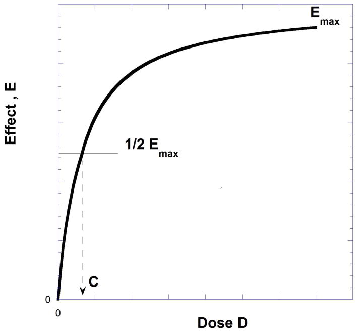
Typically, dose-response data are displayed as a graph in rectangular coordinates with the effect size plotted on the ordinate and the dose on the abscissa. This yields a monotone increasing graph that approaches the maximum effect (E_max). If the data are all-or-none, the graph is generated by plotting the percent responding on the ordinate and dose on the abscissa. Shown on Figures 9.19.1 and 9.19.2 are examples of both types of DRCs. For quantal data, it is common to calibrate the effect scale as 0–100%. For graded effects this is the maximal response to the drug, e.g. the Emax, which is denoted as 100. The dose that has an effect equal to one-half the maximum, the ED₅₀ for quantal and D₅₀ for graded curves, is displayed on Figure 9.19.1 as C. In common parlance the term ED₅₀ is used for both types of curves.

Fig. 9.19.1.

Dose-effect data often yield plotted points that are described by the hyperbolic equation E = E_max D/(D + C) that produces the smooth graph shown. The constant C (equal to dose for ½Emax) is often abbreviated ED50 or D50. It is an indicator of potency.

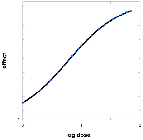
Fig. 9.19.2.

When dose-effect data are viewed on a horizontal scale with log dose, the hyperbolic curve of Figure 9.19.1 becomes sigmoidal (and approximately linear in the mid- range of effects.)

To analyze the effects of a drug combination DRCs must be generated that describe the effect of the individual agents. A common curve shape is a hyperbola that includes a defined maximum effect. If the maximum is not obvious from the plot it can be estimated using an appropriate curve fitting program (e.g., Kaleidagraph 4.5 and Graphpad Prism).

The Hyperbolic Curve

The hyperbolic curve is described by the equation

$$E=E_{\mathit{max}}D/(D+C)$$ Eqn 9.19.1

where E is the effect, D is dose and C a numerical constant (equal to the dose needed for a half-maximal response). The constant C, a measure of drug potency, is often denoted as ED₅₀ or D₅₀ (Fig. 9.19.1). The EC₅₀ or D₅₀ is used here to denote the concentration (or dose) of the test agent that produces 50% of the maximal possible response.

Equation 9.19.1, which is the most common one for describing DRCs, was initially used to describe drug receptor interactions (Clark, 1926). The graph resulting from a plot of the values generated by this equation is classified as a hyperbola.

Dose-effect curves are also displayed by plotting the response against the logarithm of the dose. This transformation yields a sigmoidal (S-shaped) curve with a nearly linear, central component (Fig. 9.19.2). When plotted in this manner the half-maximal value of the curve yields the log of C. When Emax = 100% the mid-range of this linear segment has a slope equal to 57.56. There are computer packages for curve fitting (Synergy software, Kaleidagraph 4.5; or GraphPad Prism 6.), that also calculate the constant C and its standard deviation from the generated dose-response data.

Some results require more complicated dose-response equations, e.g. Eqn. 9.19.2

$$E=\frac{E_{\mathit{max}}{D}^p}{D^p+C^p}$$ [Eqn. 9.19.2]

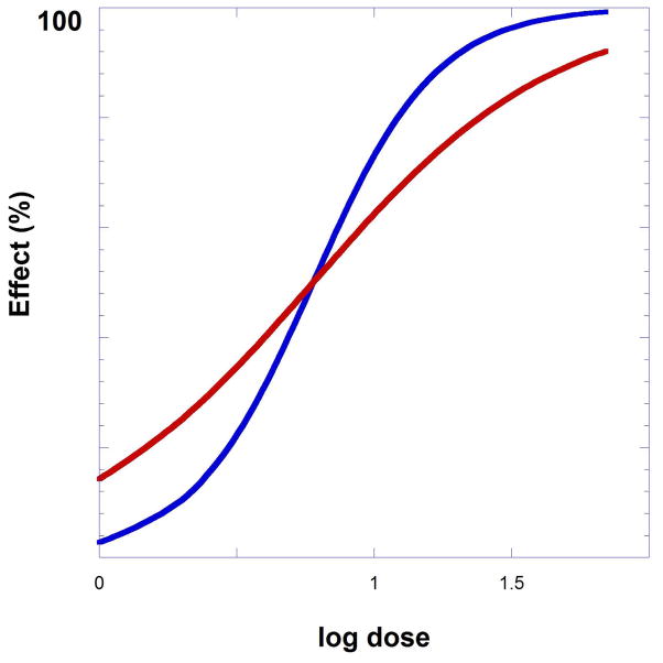
where p, the Hill coefficient (nH) is a constant. The constant p multiplies the slope of the log plot, i.e., (57.56 p) is the slope. This is illustrated on Figure 9.19.3 in which this exponent equals 2 for a set of data that graphed using results generated from Eqn. 9.19.2. It is displayed on the figure as the steeper (blue) curve. Precise dose-response data are needed for analyzing drug combination results because the drug combination study protocols and data analysis require precise knowledge of dose equivalents. For example, if drug A produces a particular effect — e.g., 50% of Emax at a dose of 30 mg, it is necessary to determine the precise dose of drug B required to produce that same response before defining the interaction of the two agents when they are administered simultaneously.

Fig. 9.19.3.

The model equation with exponent p = 2 alters the shape from the curve shown in red to the steeper curve that is colored blue. The dose-response equation of the steeper curve is given by E = E_max D²/(D² + C²)

Dose equivalence is the essential ingredient for generating isoboles and for analysis of these data. The shapes of the individual DRCs are therefore critical for determining the dose equivalence. The most basic situation is one where each drug alone attains the same maximum effect and each can be fitted to the basic hyperbolic form E = E_max D/(D + C). Generally in this case the C value for each drug is different.

The Isobole

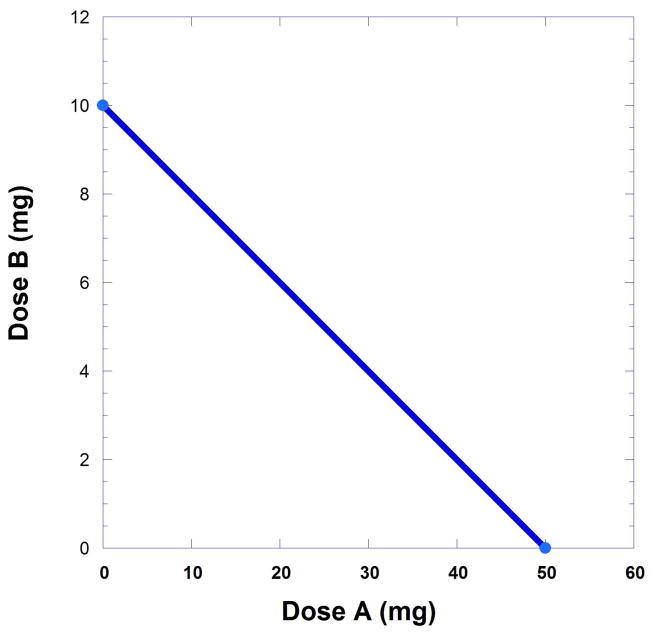
For illustration purposes, accept that experiments indicate that a certain dose of drug A yields a maximum (100 %) with ED₅₀ value if 50 mg, which is denoted as A₅₀ = 50 mg, whereas drug B displays a 100% response with an ED₅₀ value of 10 mg (B₅₀ = 10 mg). The aim is to identify a combination of doses for a and b that yields a 50% response. Such a combination can be described as the sum of the quantity b and the b-equivalent of a, which is [a(B50/A50)]. The dose of a is not simply added to the dose b. Instead, what is sought is the drug-B equivalent of dose a of drug A which is then added to the equivalent to dose b. Dose b plus this equivalent yield the B₅₀ because a total equal to B₅₀ yields 50% of the maximum response. [*To copyed: From author: Term B₅₀, like all mathematical terms, should be in italics. Also, it is best to denote the quantities a and b as doses and not use the bracketed notation that is used in chemistry for concentration.]

This is symbolized as

$$b+\left(\frac{B_{50}}{A_{50}}\right)a=B_{50}$$

This expression relates the doses that together are expected to result in a response that is 50% of the E_max. Rearrangement gives the intercept form of Eqn. 9.19.33 that is illustrated in Figure 9.19.4.

Fig 9.19.4.

An isobole of additivity derived from drugs that have ED₅₀’s values of 10 and 50 is illustrated. These ED₅₀ values constitute the axial intercepts. This line represents all dose pairs that are expected to give the specified effect (in this case 50% of E_max) and is based on the individual potencies.

$$\frac{b}{B_{50}}+\frac{a}{A_{50}}=1$$ [Eqn. 9.19.3]

It is important to note that the linear isobole expressed in Eqn. 9.19.3 is based on the fact that the dose ratio of drugs A and B is a constant and, thus, the dose equivalent in this case is $\left(\frac{B_{50}}{A_{50}}\right)a$. As demonstrated below, the isobole is curved when this constancy does not apply. The reciprocal expression of Eqn. 9.19.3 is the common form of the isobole, a straight line graph that represents all a,b combinations that will yield a particular level of response. In this case the response sought is 50% of the maximum. The isobole graph has A50 and B50 intercepts. In the illustration (Fig. 9.19.4) the values at these intercepts are 50 mg and 10 mg, respectively.

All points on the isobole represent dose pairs that when administered are expected to cause the desired effect (in this case, 50% of Emax). If experiments with a dose pair yield results that fall on the line the combined response is considered additive. That is, the drug combination acts in accordance with what was found with each agent individually. Other levels of response can be used so that instead of A50 and B50 the values of the individual doses for the targeted response, designated as A_i and B_i, are calculated. Thus, using Eqn. 9.19.3 more generally,

$$\frac{b}{B_i}+\frac{a}{A_i}=1,$$

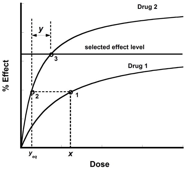
where B and A are used without subscripts with the understanding that these are the doses of each drug when used alone that produce the desired level of response. A view of the isobole derivation in relation to the individual dose-effect curves is shown on Figure 9.19.5. As this graphical view is related to the derivation it may aid in understanding the mathematics.

Fig. 9.19.5.

The additive combination (x,y) is graphically illustrated. It is seen that dose x of drug 1 has an equivalent dose of drug 2 that is denoted y_eq. When viewed as drug 2 its effect is at point 2. In order to get to the selected effect level at point 3, we need the quantity y and, thus, the pair (x,y) is a point on the isobole, and the set of all possible pair (x,y) gives the isobole graph.

It is useful to have an expression for the total in the additive combination (sum of coordinates along the isobole). This value depends on the proportions of the drugs in the combination. The proportions are denoted by p_A and p_B, with the total additive dose designated Z_add. It is given by Eqn. 9.19.4:

$$Z_{\mathit{add}}=\frac{AB}{B{p}_A+A{p}_B}$$ [Eqn. 9.19.4]

where A and B are the isobole intercepts (e.g., the ED₅₀ values if this is the usual 50% isobole). Because A and B are estimated quantities each has a variance (square of the standard error), which means there is a variance for Z_add (Eqn. 9.19.5).

$$\mathit{Var}(Z_{\mathit{add}})={\left(\frac{\mathit{Zadd}}{B}\right)}^4{p}_B^2\mathit{Var}(B)+{\left(\frac{\mathit{Zadd}}{A}\right)}^4{p}_A^2\mathit{Var}(A)$$ [Eqn. 9.19.5]

Because the isobole is an indicator of all dose combinations expected to give the desired response (e.g., 50%) it is used with the observed dose pair to determine whether there is a departure from simple additivity. Points on the line are referred to as additive because drug B and the dose B-equivalent of dose a are added together to derive the line. The isobole is linear because the dose ratio of drugs A and B is a constant. The isobole is curved when this dose ratio condition does not hold.

The dose combination example resulting in the isobole plotted on Figure 9.19.4 was based on the theoretical data illustrating the simplest type of interaction. The example shown below is based on results obtained from an actual study of the interaction of various combinations of acetaminophen and tramadol (Tallarida and Raffa, 1996).

2.3.1. Example: Tramadol + acetaminophen

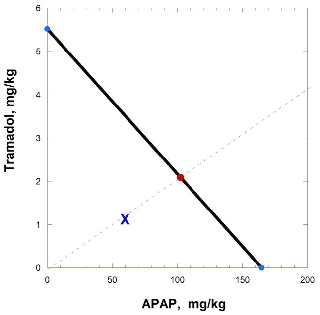
To demonstrate the application of the isobole to an actual situation we here discuss a combination study involving two well-known analgesic drugs, acetaminophen and tramadol. This study used the mouse abdominal constriction model to assess the antinociceptive actions of the two drugs. The individual dose-effect curves revealed a constant potency ratio so that the resulting isobole was linear. The acetaminophen (APAP) ED₅₀ value is denoted by A and =164.93 mg/kg p.o. with a standard error =24.5, while tramadol is designated as B with an ED₅₀ = 5.52 mg/kg p.o. and a standard error = 0.40. Combinations were tested in various proportions but we illustrate here just one of these to illustrate the calculation, viz., p_A =0.98, p_B =0.02. From Eqn. 9.19.4, Z_add = 104.5 mg/kg po with variance = 101.2 (from Eqn. 9.19.5) and thus a standard error = 10.05. (The variance calculation is shown in detail below

$$\mathit{Var}(Z_{\mathit{add}})={\left(\frac{104.5}{5.52}\right)}^4{(0.02)}^2{(0.4)}^2+{\left(\frac{104.5}{164.9}\right)}^4{(0.98)}^2{(24.5)}^2=101.2).$$

The observed total dose Z_obs = 63 mg/kg po (C.L. 50.2 – 79.0) was well below the line of additivity and is located at point (61.7, 1.26), (shown as X in Fig. 9.19.6), whereas the expected additive point is on the line at (102.4, 2.09). These data, together with similar findings at different dose ratios, indicate a synergistic interaction between the two agents. Results such as these lead to the development of the analgesic ULTRACET®.

Fig. 9.19.6.

Isobologram showing the additive (expected) and observed dose pairs of a fixed ratio combination. The position of the observed dose pair (X) below the line indicates synergism.

In summary, the standard error (in regression) is the square root of the variance, with the calculated additive total dose (which is the expected total dose) uses the graphical intercepts to derive the isobole. Because these intercepts are quantities with error all points of the isobole have error. Thus, the standard error calculation is used to compare observed points of the isobologram to the points on the additivity line. Comparisons are performed with standard statistical methods, e.g., t-distribution, that may be expressed with confidence limits.

Further Comment on Deriving the Isobole

As previously shown, when the individual drugs have a constant relative potency the isobole is linear. The isobole can still be derived even when the relative potency is not constant and the two dose-effect graphs differ. For example, consider a case where drug B displays greater efficacy than drug A and that the drug B dose that yields 50% of the maximal response is designated as B₅₀. The next step is to determine the drug B equivalent B_eq(a) of any dose a of drug A. The isobole is then described by the expression b + B_eq(a) = B₅₀. When plotted, this relationship between dose a and dose b is the additive isobole. If a different effect level for the isobole is selected, for example, level i, then the dose B_i is used for that effect instead of B₅₀. This illustrates that the isobole can be derived regardless of the shape of the individual dose-effect curves. (See section below on “Dealing with very Different Dose Effect Curves.”) In cases where the dose ratio is constant the B-equivalent of dose a is simply = a (B₅₀/A₅₀), with that quantity plus dose b yielding the linear isobole of Eqn. 9.19.3.

Experiments and Selection of the Dose Ratio of the Drug Combination

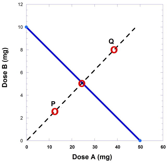
In the earlier example with drug A and drug B values leading to Figure 9.19.4, the ED₅₀ values were 50 and 10 mg, respectively. While any fixed ratio dose combination can be used for testing, very often the dose ratio selection is based on the intercept values. If, for example, dose pairs are selected that have the ratio 5 to 1 the additive dose pair for the effect level 50% is point (25, 5) (Fig. 9.19.7).

Fig. 9.19.7.

Isobologram showing points (dose combinations) that characterize the combination. Point P indicates synergism whereas point Q indicates sub-additivity. The broken line shows the dose combination ratio selected and three possible observed points for the specified effect. Point P below the line indicates synergism while point Q above the line indicates subadditivity. A point on the line is additive and means that the combination acts in accordance with the individual potencies.

A fixed ratio dose combination is selected for testing. Although any ratio can be employed, dose pairs are generally selected on the bases of the A50 and B50 (intercepts of the isobole). One such ratio would be 5:1. With this ratio the expected dose combination for a 50% effect is on the isobole at point (25, 5) (Fig. 9.19.7). The other points, labeled P and Q, are explained in the figure legend.

When the isobole of additivity is plotted and the additive dose combination determined, such as (25, 5) in this illustration, an experiment can be conducted at the dose (25, 5) to test whether the expected 50% effect is obtained. However, instead of administering the (25, 5) dose combination, it is preferable to begin with lesser quantities with this same ratio, e.g. (5, 1), (10, 2), (15,3), etc., and determine the effect of each. These experimental data (effect at each of the dose pairs) is normally plotted (effect against total combination dose) on a separate graph to obtain the total dose from the smoothed curve at the 50% effect. When that total dose is obtained it is possible to calculate the part represented by drug A and the part represented by drug B. These parts are then plotted as a point on the isobole to view its position relative to the line of additivity (Fig. 9.19.7). If the plotted point is on or near the line, the combination is said to be additive. If the observed point is below the isobole line (shown here as P) the effect represents synergism, while a point above the line (point Q) indicates sub-additivity.

When One Drug Lacks Efficacy

There are combination experiments that pair a drug with zero efficacy with one that is efficacious. An example is an ibuprofen and glucosamine combination for analgesia. Glucosamine is a naturally occurring chemical located near joints and in other parts of the human body. Glucosamine sulfate is a component of many dietary supplements, especially those recommend for arthritic patients. Ibuprofen is an established non-steroidal anti-inflammatory drug that displays antinociceptive activity in laboratory animal pain models and in humans. Glucosamine, on the other hand, displays no analgesic activity in animal tests or in humans. A combination of these two agents would yield an isobole that is a plot of ibuprofen doses on the vertical scale and glucosamine doses on the horizontal, with the resultant graph being a horizontal line at the ibuprofen dose that gives the desired effect. In other words, regardless of how much glucosamine is combined with ibuprofen, the quantity of ibuprofen needed to produce the desired analgesic effect remains the same. This is illustrated by the horizontal isobole. This combination was studied in our laboratories in the mouse abdominal constriction test (Tallarida et al., 2003). The result suggested it is possible to reduce significantly the dose of ibuprofen as the observed combination point was well below the horizontal isobole. In one of the fixed ratio combinations the ibuprofen ED₅₀ value was reduced from 26.1 ± 3.4 to 11.0 ± 2.1 (mg/kg), indicating a synergistic interaction between the two compounds.

Drugs with Different Maximum Effects

When the two drugs yield different maximum effects the dose ratio for equal effects is not a constant. For example, drug A might have a maximum that is only 60% of the maximum of drug B. The isobole is still derived from the fundamental relationship - b + B_eq(a) = B₅₀ for effect = 50% of drug B, or any desired effect of drug B. If a different effect level is used for the isobole (e.g. effect level E_i) then the dose B_i for that effect is used instead of B₅₀ on the right-hand side of this equation.

As described previously, the shape of the dose-effect curves is typically hyperbolic. In the case of two drugs having different maxima and the hyperbolic dose–effect curves are given by $E=\frac{E_{max(B)}b}{b+B_{50}}$, and $E=\frac{E_{max(A)}a}{a+A}$.

For this example drug B is designated as the compound with the greater efficacy. Therefore, B₅₀ has the usual meaning. In this situation the dose of drug A that gives half of its maximum response is denoted by A, which is not the dose for 50% of the maximum defined by E_max(B). Rather, it is the constant that describes the dose-effect curve of drug A and the dose needed to induce the half-maximal response for drug A. In this two drug situation no subscript is used with the constant A. The isobole requires the drug B equivalent of a dose a of drug A. This is denoted as B_eq(a) and is calculated from Equation 9.19.6:

$$B_{\text{eq}}(a)=\frac{B_{50}}{\left\{\frac{E_{max(B)}}{E_{max(A)}}\left[1+\frac{A}{a}\right]-1\right\}}$$ [Eqn. 9.19.6]

With simplifying notations sometimes used, e.g., Eqn. 9.19.7

$$g=\frac{E_{max(B)}}{E_{max(A)}}$$ [Eqn. 9.19.7]

so the equivalent is determined using Eqn. 9.19.8:

$$B_{\text{eq}}(a)=\frac{B_{50}}{\left\{g\left[1+\frac{A}{a}\right]-1\right\}}$$ [Eqn. 9.19.8]

If the denominator is denoted f(a) then this takes on an even simpler form (Eqn. 9.19.9):

$$B_{\text{eq}}(a)=\frac{B_{50}}{f(a)}$$ [Eqn. 9.19.9]

The isobole for the 50% effect is given by Eqn. 9.19.10:

$$b=B_{50}-\frac{B_{50}}{f(a)}$$ [Eqn. 9.19.10]

This applies to two drugs with the standard hyperbolic shape and different maxima (as above).

The isobole is derived for a level of effect of interest. It is usually the half-maximum effect of drug B (½E_max(B) which here is the compound with the greater efficacy. This designated effect of interest is obtained from the DRC for drug B using effect level E_i denoting its dose by B_i. Most often B_i is the B₅₀ because the effect of interest is usually 50% of E_max(B). The isobole follows from the equation b = B_i − B_eq(a) where B_eq(a) is from [Eqn 9.19.8] or [Eqn 9.19.9] with the B₅₀ value in the numerator even though B_i is used for effects in general.

Thus, dose b plus the dose-B equivalent of a (from drug A) equals the B_i that corresponds to the effect of interest. That equivalent is given by Eqn 9.19.6 and/or one of its alternate forms involving Eqn. 9.19.8 or Eqn. 9.19.9.

Curved Isobole

The introduction of the isobole by Loewe provided a way of analyzing drug combination data, although the graphical representation has come to overshadow the theoretical basis for this calculation. In the vast majority of cases investigators draw the graph as a straight line with intercepts equal to the individual ED₅₀ values for each agent (see examples in Figures 9.19.4, 9.19.6 and 9.19.7). However, a simple derivation shows that the isobole of additivity is often a curve. This fact was not demonstrated until the appearance of a proof in Grabovsky and Tallarida (2004), although it was mentioned, without a rigorous proof, in Loewe’s 1957 publication. Indeed, whenever the drug potency ratio varies with dose, a common occurence, the isobole is a curve. The most obvious situation of a varying relative potency is where two agonists have different E_max values. Because the shape of the additivity isobole is crucial for determining whether an observed combination point is above, on or below it, its curvature or linearity is a major factor.

This situation is discussed in detail in Grabovsky & Tallarida (2004). As an illustration a case is considered where drugs A and B have different maxima. Drug A is described by E = 40 a/(a + 50) and drug B by E = 100 b/(b + 20). The different values of Emax produce a curved isobole. Individual regression analyses gave error values of the constants: A = 50 +/ 5 and B = 20 +/ 2. The curved isobole is given by

$$b=B_{\mathit{50}}-B_{\mathit{50}}/f(a)$$

where B₅₀ is the dose 20 in this case.

$f(a)=g-1+\frac{gA}{a}$, and g = E_max(B)/E_max(A). Hence the isobole is $b=20-\frac{20}{2.5\left(1+\frac{50}{a}\right)-1}$

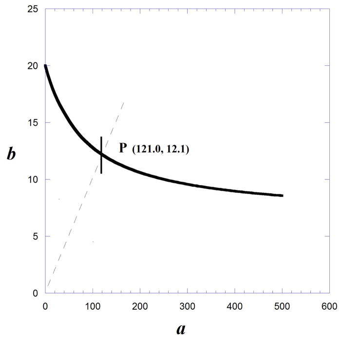
In this example, g =100/40 = 2.5 because drug A has a maximum that is 40% of the maximum of drug B. The isobole computed from Eqns. 9.19.8 to 9.19.10, and by the above equation, reveals that there is no quantity of drug A that can reduce the need for drug B to zero. That is, there is no intercept on the x-axis. The dose ratio b/a = 1/10 (shown as the broken diagonal) was selected, which defines the additive point P as a = 121.0 and b = 12.1 (Fig. 9.19.8).

Fig. 9.19.8.

Illustration of an Isobole from dose effect curves with different maximum effects: For drug B the maximum =100, while the maximum for drug A is 40. Because the selected isobole effect level is 50 it is seen that there is no intersection on the horizontal axis. This is because there is no dose of drug A that can reduce the need for drug B to zero.

The variance of b (y-coordinate on the isobole) is given by Eqn. 9.19.11.

$$\mathit{Var}(b)={\left(1-\frac{1}{f(a)}\right)}^2\mathit{Var}(B)+{\left[\frac{g}{a}\ast \frac{B}{f{(a)}^2}\right]}^2\mathit{Var}(A)$$ [Eqn. 9.19.11]

For this example the above formula for the variance of b gave 1.57. Thus, the standard error = 1.25 (square root of variance). The standard error is illustrated as the vertical segment in Figure 9.19.8. Experiments with a combination having the dose ratio 1/10 will yield the observed combination for the specified effect and its standard error. This can then be compared to the observed b-component statistically with the b value on the isobole, 12.1, and S.E. = 1.25 to detect departures from additivity.

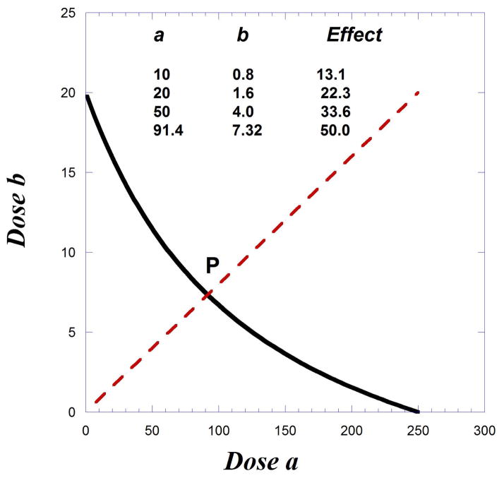
If the maximum of drug A is 60% of the Emax, the isobole would still be curved but would have an x-intercept as shown on Figure 9.19.9. The doses for 50% are the intercepts, 250 and 20. If the experiment uses a fixed ratio combination related to these intercepts, then the “path” indicated by the broken radial line has the equation b = (20/250)a. That is, the amounts of b to a maintain this ratio. The intersection of this radial line with the isobole is at point (91.4, 7.31). In other words, a combination in this dose ratio would require these doses to evoke a 50% response, the interaction is additive. The concept of dose equivalence allows a calculation of other (lesser) combination doses and the effect expected, with some of these shown in the accompanying table. Synergism is indicated if any of the lesser doses are found to produce a 50% response.

Fig. 9.19.9.

Illustration of a curved isobole (for 50% effect level) and the path (broken line) representing dose pairs (a,b) and the expected effect level of each as we approach the 50 % effect (intersection at point P). This is merely one path. Each fixed ratio dose combination gives a different path. See text.

Example: Curved Isobole

Another example of a curved isobole is where the concavity is downward rather than upward. This occurs with two drugs having the following dose-effect equations:

$$E_B=\frac{78.6b^{0.303}}{b^{0.303}+{(0.0340)}^{0.303}}\text{and}{E}_A=\frac{48.68a}{a+4.7}$$ [Eqn. 9.19.12]

In general the two dose-effect equations have the curve-fitting exponents, p on dose b and q on dose a, as shown in Eqn [9.19.13].

$$E_B=\frac{E_{\mathit{Bmax}}{b}^p}{b^p+{B_{50}}^p};E_A=\frac{E_{\mathit{Amax}}{a}^q}{a^a+A^q}$$ [Eqn. 9.19.13]

Equation 9.19.13 reminds the reader of the general case where each has an exponent. But in this example the exponent q = 1 (i.e., the exponent on dose a is one).

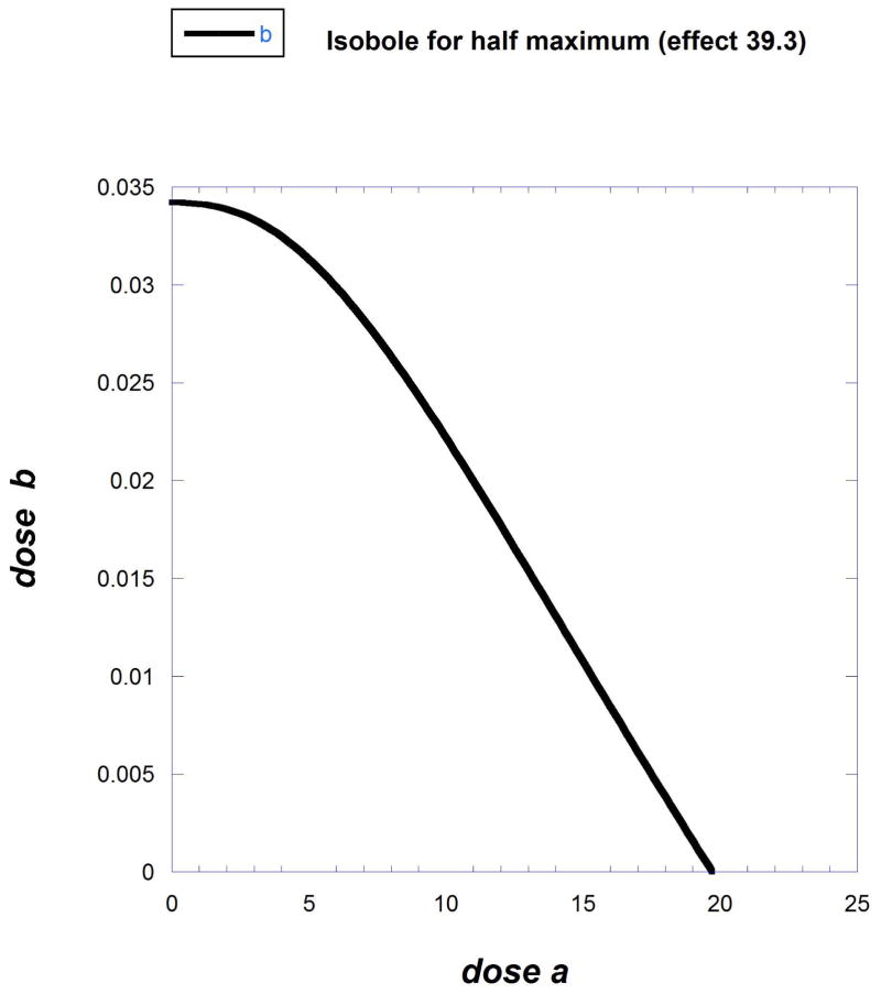
The isobole effect level selected for drug B is 39.3 (half the maximum of the higher efficacy compound). This example illustrates that isoboles can have various shapes. The general isobole equation provided below (Eqn. 9.19.14) describes the situation where exponent q is 1 and A (the half maximal response dose of drug A) is 4.7.

$$b=B_{50}-\frac{B_{50}}{{\left\{\frac{\mathit{Emax}(B)}{\mathit{Emax}(A)}\left[1+\frac{A^q}{a^q}\right]-1\right\}}^{1/p}}$$ [Eqn. 9.19.14]

Other values to insert in the Eqn. 9.19.14 are B₅₀ = 0.0340, Emax(B) = 78.6, Emax(A) =48.68, P = 0.303, q = 1 and A = 4.7. These values give the isobole for effect 39.3 (Fig. 9.19.10). Another example yielding this type of isobole is given by data obtained when combining cocaine and remifentanil, as described below.

Fig. 9.19.10.

A curved isobole derived from a study in which one of the dose response equations contains the exponential term (see Eqn [12]) as part of the b dose.

Example #1: Cocaine and remifentanil

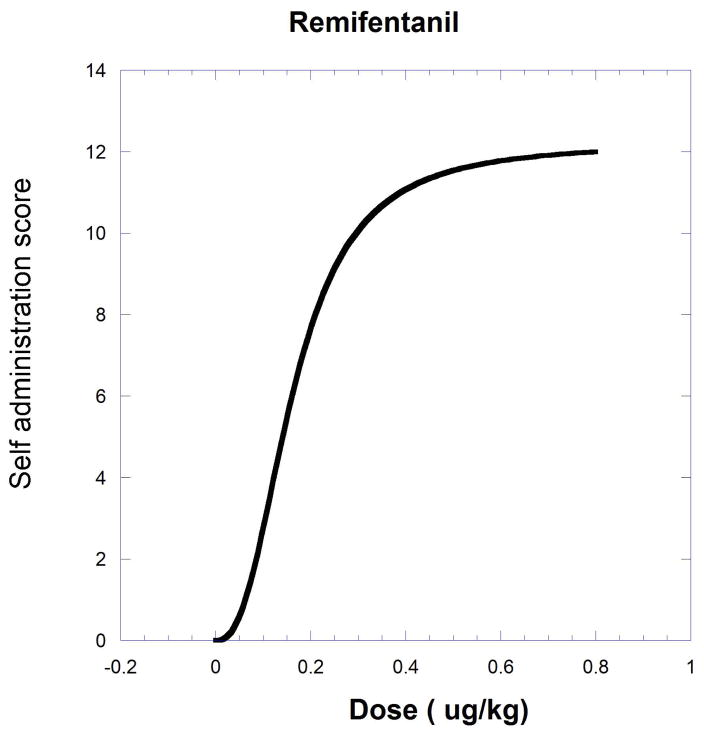
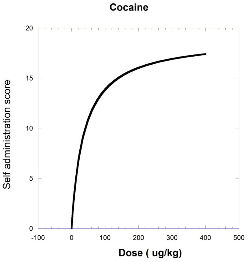
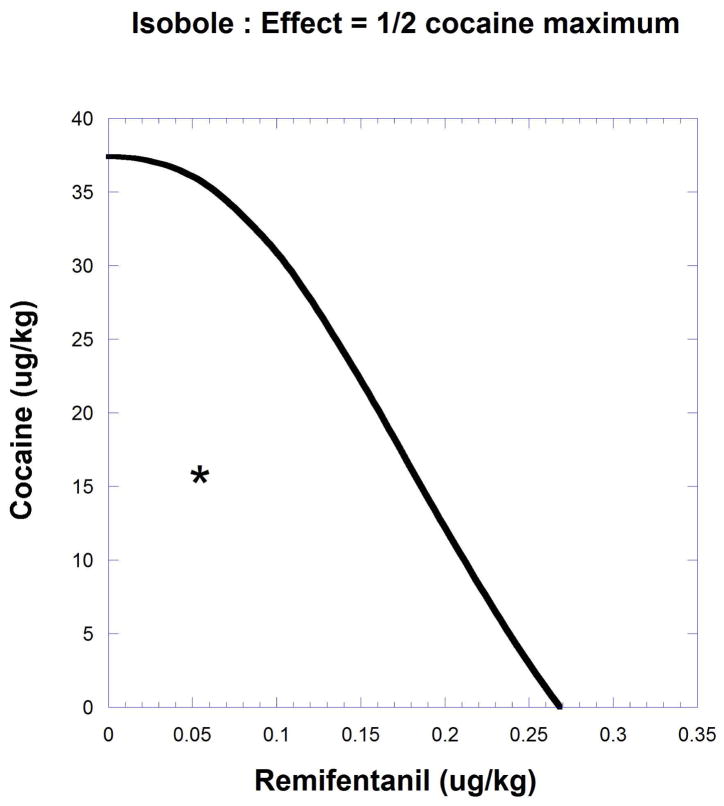
The next example, producing a curved isobole, uses data from the study of cocaine and remifentanil by Woolverton et al. (2008). It is based on a drug self-administration procedure that recorded the number of injections (in monkeys). The dose-response equations that apply are given in the legend to Figure.9.19.11 and in Eqn. 9.19.15.

Fig. 9.19.11.

A self-administration score (determined from injections per session) in monkeys is shown as smoothed dose-effect curves for remifentanil (upper) and cocaine (lower). Equations from nonlinear regression are for remifentanil $E=\frac{12.2D^{2.53}}{D^{2.53}+{0.163}^{2.53}}$, and for cocaine $E=\frac{19.02D}{D+37.4}$. The effect = one half the cocaine maximum (9.51) is used to derive the isobole shown in Figure 9.19.12. The isobole for effect 9.51 is derived by substitution with the drug pair parameters and is given below to show the calculation detail. This form of the isobole Eq. [14] has p = 1 and q = 2.53.

$$b=37.4-\frac{37.4}{{\left\{\frac{19.02}{12.2}\left[1+{\left(\frac{.163}{a}\right)}^{2.53}\right]-1\right\}}^1}$$ [Eqn. 9.19.15]

Example #2: A set of curved isoboles

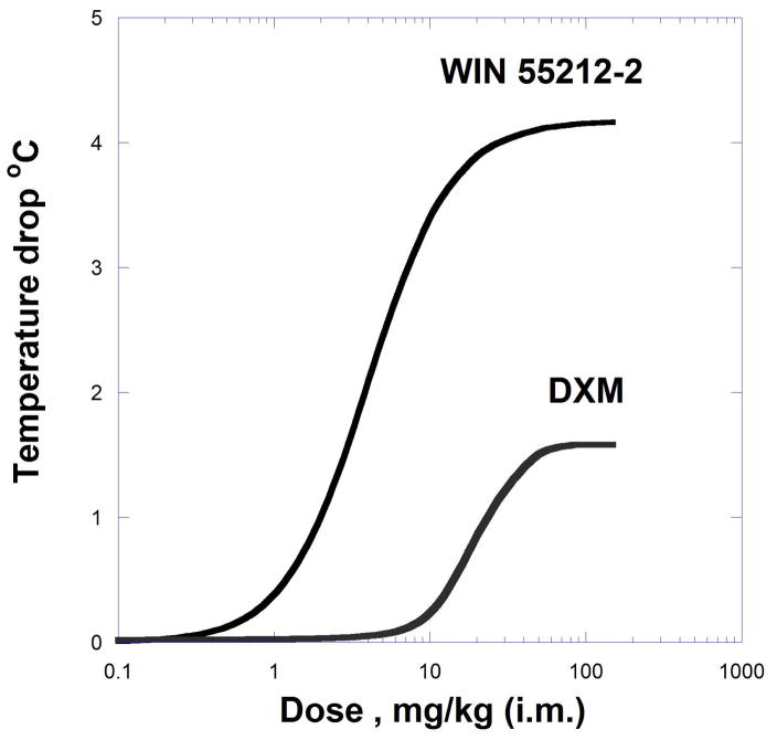
Dose-response curves for drugs with different maxima and the corresponding isobole combination are exemplified by the ability of dextromethorphan (an NMDA antagonist) and WIN 5521202, a cannabinoid agonist, to decrease body temperature in rats (Rawls et al., 2002; Grabovsky and Tallarida, 2004).

Because the curves (Fig. 9.19.13) of the individual compounds are not well described by simple hyperbolas, they were fitted by equations that contained exponents:

Fig. 9.19.13.

Dose-effect curves for the decrease in body temperature produced by DXM and WIN 55212-2. These were derived using curve-fitting parameters (exponents p and q) as described in the text. Data from Rawls et al (2002} and used in Grabovsky & Tallarida (2004) with permission.

E = E_maxB b^p/(b^p + B₅₀^p) for WIN55212-2 with E_maxB = 4.17, p = 1.73, and B₅₀ = 3.99, and fitted to E = E_maxA a^q/(a^q + A^q) with E_{max A)} = 1.58, q = 1.92 and A = 65.8 for dextromethorphan. In this case, in which exponents (p and q) are needed for the dose-effect equations, Eqn 9.19.16 describes the isobole of additivity. Recall that the second term on the right is Beq(a). From this equation, a set of additive isoboles are obtained for the specified effect levels (temperature drop in °C).

$$b=B_i-\frac{B_{50}}{{\left\{\frac{\mathit{Emax}(B)}{\mathit{Emax}(A)}\left[1+\frac{A^q}{a^q}\right]-1\right\}}^{\frac{1}{p}}}$$ [Eqn. 9.19.16]

A calculation using this equation and the above curve-fit values follows. Note that Eqn. 9.19.16 closely resembles Eqn. 9.19.12, although Eqn. 9.19.16 is a bit more general in that B_i is a dose that is more general than B₅₀ since B_i is for the selected i-level effect.

The isoboles for selected effect levels (temperature decrease) for the drug combination are displayed on Figure 9.19.14 and calculated below using Eqn. 9.19.16. For i.m. doses of WIN 55212-2 greater than 3 mg/kg the isobole of additivity is an unbounded arc that approaches a horizontal asymptote. A representative calculation shows the isobole equation for effect level 2 by substitution in Eqn. [9.19.16]. The value 3.81 shown in Eqn 9.19.17 is the B_i dose of compound B (WIN 55212-2) that alone yields an effect = − 2°C.

Fig. 9.19.14.

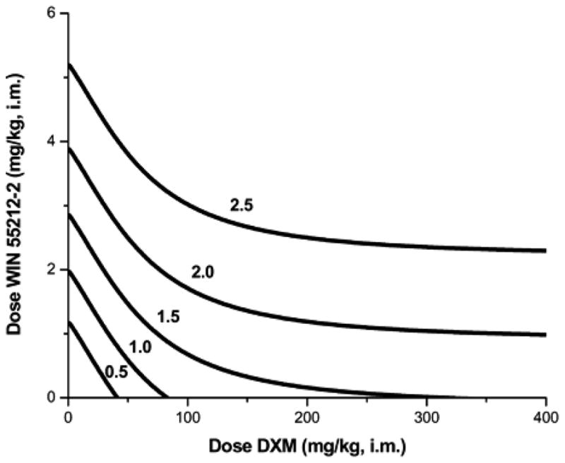
Isoboles for several different effect levels, where the effect is magnitude of the decrease in temperature (°C) in rat due to the combination of dextromethorphan (DXM) and WIN 55212-2. Because DXM alone has a maximum effect = 1.58, the isoboles for effect levels 2.5 and 2.0 have no intercepts on the horizontal axis.

$$b=3.81-\frac{3.99}{{\left\{\frac{4.17}{1.58}\left[1+\frac{{65.8}^{1.92}}{a^{1.92}}\right]-1\right\}}^{\frac{1}{1.73}}}$$ [Eqn. 9.19.17]

This example demonstrates that a very clear drug effect yields a set of curved isoboles and some of these have no intercept on the x-axis (see Fig. 9.19.14). This is very different from the erroneous belief that the additive isobole is always linear. This example also illustrates that an isobole can be derived for any effect between 0 and E_max., although the 50% level is most common.

Site-Site Analysis

While the main focus of this unit is drug combinations, the model equations and associated methodology are also applicable as well for assessing the effects of a single drug that acts at two sites. As an example, brain/spinal-cord interactions for acetaminophen-induced antinociception were tested using the mouse abdominal constriction assay (Raffa et al., 2000). Acetaminophen was administered intrathecally to mice at a dose that produced dose-related, antinociception with an ED₅₀ value of 137 (S.E. = 23) μg. However, little or no effect was observed when acetaminophen was administered directly into brain at doses up to 150 μg. Combined administration of acetaminophen in fixed ratios to brain and spinal cord, however, displayed a synergistic antinociception, with a reduction in the ED₅₀ from 137 to 57 μg (S.E. = 9) for the intrathecal dose.

OPPOSITE EFFECTS

Combinations of agonists that produce opposite effects

There is continuing interest in drugs of abuse on the immune system and on infection. Certain pairs used together produce opposite effects. For example, treatments with WIN 55, 212,-2 can produce hypothermia while a lipopolysaccharide component of Gram-negative bacteria induces fever. The use of combinations of these therefore requires an analysis of this kind of situation, one in which the compounds exert opposite effects, thereby further advancing the theory. Situations in which two agonists produce opposite effects include those where one drug might be used to treat some other condition or when there is an endogenous chemical having an effect that is opposite to that of a therapeutic or illicit compound. This issue was examined by studying the response to two compounds with opposite thermal effects, a lipopolysaccharide (LPS) which induces fever and a cannabinoid that causes hypothermia (Benamar et al., 2007). The results of this analysis are detailed in the cited publication. The equations utilized are very similar to those described in this unit.

Very Different Dose-Effect Curves

Situations are sometimes encountered where the dose-response relationship of one or both of the drugs does not conform to the usual hyperbolic curve. As an example, consider two drugs with dose-effect curves as follows:

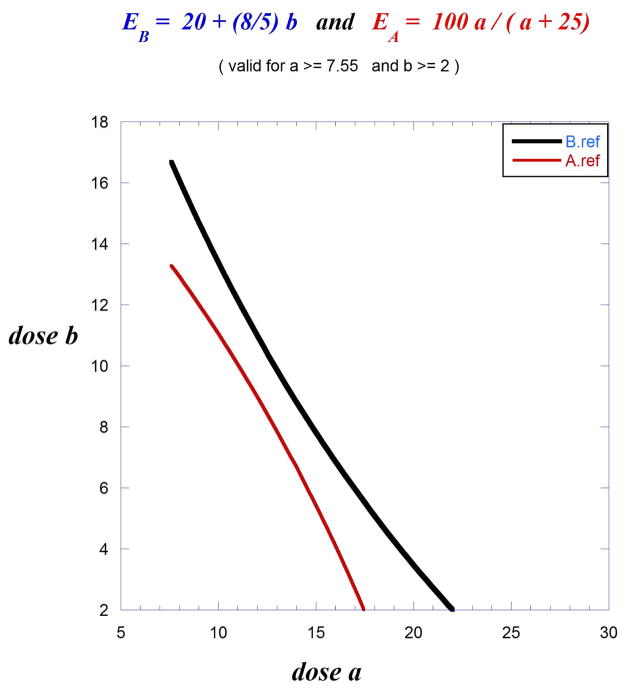
E_A = 100 a/(a + 25), which is hyperbolic, and E_B = 20 + 1.6 b, which is linear. (b > = 2).

Drug A, with a dose denoted a, generates the standard hyperbolic form, whereas drug B, with dose b, is linear. The E_A and E_B equations reveal that A₅₀ = 25 and B₅₀ = 18.75. Also, each drug attains the 100% effect level. Some dose-response equations may be restricted to certain dose ranges, as in this case where b must be greater than 2 so that correspondingly a > 7.55. It is not clear whether the additivity analysis should use doses of drug A equivalent to drug B or doses of drug B equivalent to drug A. It is best to test both instances.

The equal-effect expression is 20 + 1.6 b = 100 a/(a + 25), which holds for a > 7.55, b > 2. The drug-B equivalent of dose a is initially obtained by solving for b in terms of a:

$$b_{eq}(a)=\frac{80a-500}{1.6a+40}$$

The isobole for the 50% effect is defined as b + b_eq(a) = 18.75 and, from the above, this yields the $\mathit{isobole}b=18.75-\frac{80a-500}{1.6a+40}$.

The drug-A equivalent of dose b can then be calculated by solving for a in terms of b. This gives

$$a_{eq}(b)=\frac{40b+500}{80-1.6b}\text{and}\text{from}\text{it},\text{the}\text{other}50\%\text{isobole}:a=25-\frac{40b+500}{80-1.6b}$$

These can be re-written such that each expresses b in terms of a which makes possible an informative graphical display of both isoboles on the same set of axes (Fig. 9.19.15). This dual isobole situation is problematic for comparing additivity with synergism. A reasonable approach is to consider the space between the two isoboles as a region of additivity with, therefore, any departure (such as synergism or sub-additivity) being represented by points outside the additivity region.

Fig. 9.19.15.

The individual dose effect curves lead to two isoboles (50% effect level) because the individual curves do not have a constant dose ratio and therefore either is used to predict additivity from the dose-equivalence procedure. (See text). The upper curve is based on the use of drug B as the reference drug for deriving the isobole.

SUMMARY and DISCUSSION

While this unit deals primarily with the isobole and its basis in the concept of dose equivalence, other approaches may be used to assess drug interactions (Tallarida, 2006 and 2012; tallarida and Raffa, 2010). An alternative method proposed by Chou and Talalay (1984) is based on kinetic principles that, according to the authors, is more general than the isobole procedure. Another approach is sometimes described as the “Bliss independence model” (Bliss, 1939). In this case a simple calculation is made to determine the fractional effect of dose a of drug A and dose b of drug B. On an effect scale of 0 to 100, Bliss gives the formula below for calculating the fractional effect of the combination F_ab in terms of fractional effects of drug A and drug B:

$$F_{ab}=F_a+F_b\_F_a\ast F_b$$

Bliss did not give a mathematical derivation and did not otherwise justify the use of this equation except to state that it is based on an old formula used in entomological studies for assessing toxic interaction of combinations of poisons. However, the Bliss formula is not compatible with the isobole approach (see Tallarida, 2012).

It has been demonstrated that the isobole can be either a straight or a curved line. It is always linear when the individual dose-effect curves have a constant potency ratio, and curved when the ratio is variable. While Loewe appreciated this fact it was not accepted by Berenbaum (1989) who incorrectly asserted that isoboles are straight lines. Berenbaum’s proof used as the two compounds a real drug and a diluted form of the same substance. The fact that he found this combination results in linearity is not surprising in that the two substances are actually the same drug at different concentrations, which is bound to yield a constant potency ratio and therefore a linear isobole. As shown in this unit, the Berenbaum theory does not necessarily hold for the more standard drug combinations that involve two different chemical substances. Provided in this unit are examples of compound combinations that yield curved isoboles to illustrate this important point.

The two essential equations that apply when the individual dose-effect curves are hyperbolic forms with Hill coefficient, exponent p for drug B and exponent q for drug A are shown below. Eqn 9.19.17 is used when the isobole effect level is 50% E_max, and Eqn 9.19.18 when the isobole effect level is another level with a half-maximum dose of B_i. In each case, term A is the dose of drug A that gives half of its own maximum.

$$b=B_{50}-\frac{B_{50}}{{\left\{\frac{\mathit{Emax}(B)}{\mathit{Emax}(A)}\left[1+\frac{A^q}{a^q}\right]-1\right\}}^{1/p}}$$ [Eqn. 9.19.17]

$$b=B_i-\frac{B_{50}}{{\left\{\frac{\mathit{Emax}(B)}{\mathit{Emax}(A)}\left[1+\frac{A^q}{a^q}\right]-1\right\}}^{\frac{1}{p}}}$$ [Eqn. 9.19.18]

Fig. 9.19.12.

The intercepts represent the respective doses 37.4 and 0.267 (ug/kg) for cocaine and remifentanil that individually gave effect = 9.51 (1/2 the cocaine maximum). The isobole is curved because the individual drug maxima and the exponent in remifentanil’s dose-effect equation lead to a varying potency ratio for these drugs. Experimentally a combination dose that gave this effect was found to be approximately (0.05, 16), a point (*) below the isobole, thereby indicating synergism.

Literature Cited

- Benamar K, Yondorf M, Meissler J, Geller E, Tallarida RJ, Eistenstein T, Adler MW. A novel role of cannabinoids: implications in the fever-induced by bacterial lipopolysaccharides. J Pharmacol Exp Ther. 2007;320:1127–1133. doi: 10.1124/jpet.106.113159. [DOI] [PubMed] [Google Scholar]
- Berenbaum MC. What is Synergy? Pharmacol Rev. 1989;41:93–144. [PubMed] [Google Scholar]
- Bliss CI. The toxicity of poisons applied jointly. Ann Appl Biol. 1939;26:585–615. [Google Scholar]
- Gessner PK, Cabana BE. A study of the hypnotic and of the toxic effects of chloral hydrate and ethanol. J Pharmacol Exp Ther. 1970;174:247–259. [PubMed] [Google Scholar]
- Chou TC, Talalay P. Quantitative analysis of dose-effect relationships: the combined effects of multiple drugs or enzyme inhibitors. Adv Enz Regul. 1984;22:27–55. doi: 10.1016/0065-2571(84)90007-4. [DOI] [PubMed] [Google Scholar]
- Clark AJ. The relation between acetylcholine and muscle cells. J Physiol. 1926;61:530–546. doi: 10.1113/jphysiol.1926.sp002314. [DOI] [PMC free article] [PubMed] [Google Scholar]
- Grabovsky Y, Tallarida RJ. Isobolographic analysis for combinations of a full and partial agonist: curved isoboles. J Pharmacol Exp Ther. 2004;310:981–986. doi: 10.1124/jpet.104.067264. [DOI] [PubMed] [Google Scholar]
- Loewe S. Die Mischiarnei Klin. Wochenschr. 1927;6:1077–1085. [Google Scholar]
- Loewe S. Die quantitativen Probleme der Pharmakologie. Ergebn Physiol. 1928;27:47–187. [Google Scholar]
- Loewe S. The problem of synergism and antagonism of combined drugs. Arzneimittelforschung. 1953;3:285–290. [PubMed] [Google Scholar]
- Loewe S. Antagonism and Antagonists. Pharmacol Rev. 1957;9:237–242. [PubMed] [Google Scholar]
- Raffa RB, Stone DJ, Tallarida RJ. Discovery of “self-synergistic” spinal/supraspinal antinociception produced by acetaminophen (paracetamol) J Pharmacol Exp Ther. 2000;295:291–294. [PubMed] [Google Scholar]
- Rawls SM, Cowan A, Tallarida RJ, Geller EB, Adler MW. NMDA antagonists and WIN 55212-2, a cannabinoid antagonist, interact to produce synergistic hypothermia. J Pharmacol Exp Ther. 2002;303:395–402. doi: 10.1124/jpet.102.037473. [DOI] [PubMed] [Google Scholar]
- Tallarida RJ, Raffa RB. Testing for synergism over a range of fixed ratio drug combinations: Replacing the isobologram. Life Sciences. 1996;58:PL23–28. doi: 10.1016/0024-3205(95)02271-6. [DOI] [PubMed] [Google Scholar]
- Tallarida RJ, Cowan Alan, Raffa Robert B. Antinociceptive Synergy, Additivity, and Subadditivity with Combinations of Oral Glucosamine Plus Nonopioid Analgesics in Mice. J Pharmacol Exp Ther. 2003;307:699–704. doi: 10.1124/jpet.103.054320. [DOI] [PubMed] [Google Scholar]
- Tallarida RJ. An overview of drug combination analysis with isobolograms. Perspectives in Pharmacology. J Pharmacol Exp Ther. 2006;319(1):1–7. doi: 10.1124/jpet.106.104117. [DOI] [PubMed] [Google Scholar]
- Tallarida RJ, Raffa RB. The application of drug dose equivalence in the quantitative analysis of receptor occupation and drug combinations. Pharmacol & Ther. 2010;127:165–174. doi: 10.1016/j.pharmthera.2010.04.011. [DOI] [PMC free article] [PubMed] [Google Scholar]
- Tallarida RJ. Revisiting the Isobole and Related Quantitative Methods for Assessing Drug Synergism, Perspective in Pharmacology. J Pharmacol Exp Ther. 2012;342:2–8. doi: 10.1124/jpet.112.193474. [DOI] [PMC free article] [PubMed] [Google Scholar]
- Woolverton WL, Wang Zhixia, Vasterling Theresa, Tallarida Ronald J. Self-administration of cocaine-remifentanil mixtures by monkeys: an isobolographic analysis. Psychopharmacol. 2008;198:387–394. doi: 10.1007/s00213-008-1152-5. [DOI] [PMC free article] [PubMed] [Google Scholar]