ConvexLAR: An Extension of Least Angle Regression

Abstract

The least angle regression (LAR) was proposed by Efron, Hastie, Johnstone and Tibshirani (2004) for continuous model selection in linear regression. It is motivated by a geometric argument and tracks a path along which the predictors enter successively and the active predictors always maintain the same absolute correlation (angle) with the residual vector. Although it gains popularity quickly, its extensions seem rare compared to the penalty methods. In this expository article, we show that the powerful geometric idea of LAR can be generalized in a fruitful way. We propose a ConvexLAR algorithm that works for any convex loss function and naturally extends to group selection and data adaptive variable selection. After simple modification it also yields new exact path algorithms for certain penalty methods such as a convex loss function with lasso or group lasso penalty. Variable selection in recurrent event and panel count data analysis, Ada-Boost, and Gaussian graphical model is reconsidered from the ConvexLAR angle.

1 Introduction

Regularization is a tool to avoid overfitting and obtain parsimonious and interpretable models, especially when the number of parameters exceeds the number of observations. One powerful regularization technique is penalization. In general, a penalty method minimizes the sum of a loss function and a penalty term. The simplest ℓ₁ penalty leads to the popular lasso regression (Tibshirani, 1996; Donoho and Johnstone, 1994). Various other penalty methods have been developed thereafter. Each one targets on a specific question that arises in applications. For instance, the group penalty (Yuan and Lin, 2006; Meier et al., 2008) aims to select groups of variables such as in factorial data analysis. The adaptive lasso (Zou, 2006) applies a weighted penalty method in a data driven fashion that improves the asymptotic properties. All these penalty methods are formulated as an optimization problem and the solution is obtained by either optimizing at a grid of tuning parameter values or by a path algorithm that tracks the solution as a function of the tuning parameter.

In contrast to penalty methods, the least angle regression (LAR) proposed by Efron et al. (2004) is purely motivated by a geometric argument rather than optimization. Given a response vector y = (y₁, y₂,⋯, y_n)^T ∈ IRⁿ and its corresponding design matrix X = (x₁, …, x_n)^T ∈ IR^n×p with x_i = (x_i1, x_i2,⋯, x_ip)^T, let 𝒜_t be the active index set at time t. Following Efron et al. (2004), we assume that the covariates x^(j) = (x_1j, x_2j, …, x_nj)^T have mean 0 and unit length, and that the response y has mean 0. At t = 0, β(0) = 0_p and 𝒜₀ contains the predictor that is most correlated with the response vector y. At any t > 0, regression coefficients of active predictors, namely β_j(t) for j ∈ 𝒜_t, move along a direction such that their corresponding predictor vectors x^(j) share the same absolute correlation (angle) with the residual vector e(t) = y−Xβ(t). Here the correlation is nothing but the scaled score vector of the least squares criterion with entries

$$-\frac{1}{2}\frac{\partial }{\partial {\beta }_j}\sum _{i=1}^n{{(y_i-{\mathit{x}}_i^{\top }\mathit{\beta })}^2|}_{\mathit{\beta }=\mathit{\beta }(t)}.$$

LAR has gained wide popularity since its introduction. However, there seem only a few attempts for generalizations, strikingly unparallel to the fast development of penalty methods. Specific versions of group LAR for least squares problem are mentioned in Yuan and Lin (2006) and Park and Hastie (2006). Wu extends LAR to the generalized linear models (Wu, 2011) and the Cox’s proportional hazard model (Wu, 2012). In this article, we demonstrate that the powerful geometric idea of LAR can be generalized in a fruitful way and leads to potentially many more applications.

The remaining of the paper is organized as follows. In Section 2, we derive a basic ConvexLAR algorithm that performs continuous variable selection for any general convex loss functions. For least squares loss, Efron et al. (2004) show that the LAR solution path is piecewise linear. This leads to their efficient path following algorithm with computational cost of a single ordinary least squares estimation. For a general loss function, the piecewise linearity property is lost. However, it can be shown that the solution path is piecewise smooth and, within each path segment, follows a simple ordinary differential equation (ODE). ConvexLAR tracks the solution path by utilizing the rich numerical resource for solving ODE. Just like the original LAR for least squares, a simple modification of ConvexLAR yields the corresponding lasso solution path.

In Section 3, we show that the geometric idea of LAR can be adapted to various situations. We demonstrate this by incorporating data adaptive weights and group selection into the ConvexLAR algorithm. Comparing to their penalization analogs, these extensions avoid repeated optimizations and are computationally attractive. Moreover, a slight modification of ConvexLAR yields the exact solution path for the corresponding penalization method. ConvexLAR and its extensions are illustrated by various numerical examples in Section 4. To the best of our knowledge, no LAR algorithms have been proposed for these examples in the current literature. Finally we conclude with a brief discussion.

2 ConvexLAR Algorithm and ConvexLASSO Modification

In this section, we derive the ConvexLAR algorithm which forms the basis of various extensions presented in the next section. The algorithm is similar to the LAR algorithms developed for GLM and Cox model (Wu, 2011, 2012) but with much more generality and simpler derivation. We consider an arbitrary strictly convex loss function f(β), where β ∈ IR^p is the vector of parameters subject to regularization. ∇f(β) = [∇₁f(β), …, ∇_pf(β)]^T ∈ IR^p denotes the gradient vector of the loss function and H(β) = d²f(β) ∈ IR^p×p the Hessian, where ∇_jf(β) denotes the partial derivative of f(β) with respect to β_j for j = 1, …, p. When f is a negative log-likelihood function, ∇f(β) equals the negative of the score vector and H(β) is the observed information matrix. We use t to index the LAR solution path, with the solution at any t denoted by β(t). The active index set at t is denoted by 𝒜_t. For notational simplicity, we will drop the subscript t whenever it is obvious from the context. For instance, β_𝒜(t) and ∇_𝒜f(β) are the subvectors of β(t) and ∇f(β) corresponding to active predictors at t respectively. Similarly, H_𝒜(β(t)) is the submatrix of the Hessian corresponding to 𝒜_t.

The key idea of LAR (Efron et al., 2004) is to move the solution in a direction such that the gradient (score) corresponding to each active predictor variable has the same absolute value. We denote this common value by s(t), where s stands for the score. This prescribes that the active solution vector has to satisfy |∇_jf(β)| = sgn(∇_jf(β)) · ∇_jf(β) = s(t) or equivalently

$${\nabla }_{j}f(\mathit{\beta })-sgn({\nabla }_{j}f(\mathit{\beta }))s(t)=0,j\in {\mathcal{A}}_t.$$

Note that, for any active predictor j, ∇_jf(β) is non-zero and therefore has a constant sign, denoted by sgn(∇_jf(β)), within a segment. In vector form, we have

$${\nabla }_{\mathcal{A}}f(\mathit{\beta })-sgn({\nabla }_{\mathcal{A}}f(\mathit{\beta }))s(t)=\mathbf{0}.$$ (1)

In general s(t) can be any smooth and monotonic function that decreases from s(0) = max_j |∇_jf(0)| to s(t_max) = 0 at some finite t_max > 0. Intuitively s(t) controls how the common absolute score of active predictors decays with respect to solution index t. Different choices of s(t) lead to different indexing systems yet the same solution path. The classical LAR (Efron et al., 2004) sets s(t) = s(0) − t which implies that t_max = s(0) = max_j |∇_jf(0)|.

By construction s(t) is larger than the absolute value of the scores of inactive predictors which are packed at zero. Once the absolute score |∇_jf(β(t))| of an inactive predictor j coincides with s(t), it joins the club and its score conforms to the ruling s(t) thereafter. Whenever such an event happens, the set of active predictors is updated by adding this new predictor. The index location t corresponding to this event defines a transition point in the sense that the set of active predictors changes (Wu, 2011). A path segment is defined as the solution path between two consecutive transition points. The following result follows from the implicit function theorem and provides the path following direction of the ConvexLAR algorithm within a path segment. See the Appendix for the proof and the following subsection for the definition of path segment operationally.

Theorem 1

For a strictly convex and twice differentiable loss function f(β), the LAR path solution β(t) is continuous and differentiable at t within a path segment. In addition, the solution vector β(t) satisfies the ordinary differential equation

$$\frac{d}{dt}{\mathit{\beta }}_{\mathcal{A}}(t)=s^{\prime }(t){\mathit{H}}_{\mathcal{A}}^{-1}(\mathit{\beta })sgn({\nabla }_{\mathcal{A}}f(\mathit{\beta }(t)))$$ (2)

and β_j(t) = 0 for any j ∉ 𝒜_t.

2.1 ConvexLAR Algorithm

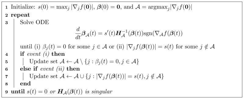
Theorem 1 suggests that the exact solution path of LAR can be obtained by solving the simple ODE system (2) segment by segment. The size of the ODE system within a segment is equal to the corresponding number of active predictors |𝒜|. The ConvexLAR algorithm is summarized in Algorithm 1. We initialize our solution path with β(0) = 0 and the beginning active set contains the predictors that change the objective function f(0) fastest. That is

$${\mathcal{A}}_0=\{{\text{argmax}}_j\mid {\nabla }_{j}f(\mathbf{0})\mid \}.$$

Algorithm 1.

ConvexLAR.

We then follow the solution path by solving the ODE system (2) until one or more new variables join the active set at some t₁ > 0, which is determined by the moment the active score s(t) matches the maximum (absolute) gradient of one or more non-active predictors. The active predictor set 𝒜_t stays the same within t ∈ [t₀, t₁). At t₁, it is updated by adding the new predictors that newly join the club. This process continues segment by segment until all the predictors are active. Then, in the final segment, the ConvexLAR solution path moves along a direction such that the absolute values of the first-order partial derivatives decrease at the same speed to zero, which happens at t_max. Under assumptions of Theorem 1, the solution β(t_max) is the global minimizer of the convex loss function, just like the LAR solution ends at the full ordinary least squares estimate. This completes our ConvexLAR solution path algorithm.

2.2 Remark

In this section, we make the following four remarks on the ConvexLAR algorithm.

Remark 1

For the specific choice of s(t) = s(0) − t,

$$t_1=s(0)-s(t_1)=\left(\underset{j^{\prime }}{max}\mid {\nabla }_{j^{\prime }}f(\mathbf{0})\mid \right)-\mid {\nabla }_{j}f(\mathit{\beta }(t_1))\mid$$

for any j ∈ 𝒜_t1. This holds analogously for later transition points. At the end of the m-th LAR segment, the transition point

$$t_m=\left(\underset{j^{\prime }}{max}\mid {\nabla }_{j^{\prime }}f(\mathbf{0})\mid \right)-\mid {\nabla }_{j}f(\mathit{\beta }(t_m))\mid$$

for any j ∈ 𝒜_tm.

Remark 2

For least squares problems, the loss is a quadratic function $f(\mathit{\beta })={\Vert \mathit{y}-\mathit{X}\mathit{\beta }\Vert }_2^2/2$ with a constant Hessian matrix H(β) = X^TX. Since sgn(∇_jf(β(t))) is constant for all j ∈ 𝒜_t in a neighborhood of t, ${\mathit{H}}_{\mathcal{A}}^{-1}(\mathit{\beta })sgn({\nabla }_{\mathcal{A}}f(\mathit{\beta }(t)))$ in (2) is piecewise constant. This leads to the piecewise linear solution path of the original LAR (Efron et al., 2004).

Remark 3 (Non-strictly convex losses)

The strict convexity assumption on the loss f precludes applications with non-convex losses or the n < p least squares case. However from the proof in Appendix, we observe that the only essential ingredient is the positive definiteness of H_𝒜(β(t)). Therefore in non-strictly convex cases, we terminate path following as soon as H_𝒜(β(t)) becomes singular.

Remark 4 (Partial regularization)

So far we have assumed that the full set of parameters β are subject to regularization. In many applications, only a subset of parameters are regularized. Assume that the loss takes the form f(β₀, β), where β₀ ∈ IR^p₀ is the vector of parameters exempt from regularization. Depending on the objective function, it may not be easy to remove β₀ from the objective. However we can always define the marginal minimizer of β₀ as a function of β

$${\mathit{\beta }}_0(\mathit{\beta })={\text{argmin}}_{{\mathit{\beta }}_0}f({\mathit{\beta }}_0,\mathit{\beta }).$$ (3)

Assume that f is strictly convex and thrice differentiable, then this mapping is uniquely defined and twice differentiable by the implicit function theorem. Denote the Jacobian and Hessian of this mapping by Dβ₀(β) ∈ IR^p₀×p and Hβ₀(β) ∈ IR^p₀p×p respectively. Then the first two derivatives with respect to β required in Theorem 1 can be obtained by the chain rule

$$\begin{array}{ll}\hfill \nabla f(\mathit{\beta })& ={\nabla }_{\mathit{\beta }}f({\mathit{\beta }}_0,\mathit{\beta })+{\nabla }_{{\mathit{\beta }}_0}f({\mathit{\beta }}_0,\mathit{\beta })·D{\mathit{\beta }}_0(\mathit{\beta }),\\ \hfill Hf(\mathit{\beta })& =d_{\mathit{\beta },\mathit{\beta }}^{2}f({\mathit{\beta }}_0,\mathit{\beta })+D{\mathit{\beta }}_0{(\mathit{\beta })}^{\top }·d_{{\mathit{\beta }}_0,{\mathit{\beta }}_0}^{2}f({\mathit{\beta }}_0,\mathit{\beta })·D{\mathit{\beta }}_0(\mathit{\beta })+[d_{{\mathit{\beta }}_0}f({\mathit{\beta }}_0,\mathit{\beta })\otimes {\mathit{I}}_p]H{\mathit{\beta }}_0(\mathit{\beta }).\end{array}$$

The Ada-Boost and Gaussian graphical model examples in Section 4 illustrate this strategy.

2.3 ConvexLASSO Modification

Efron et al. (2004) showed that in the least squares case the lasso solution path can be obtained by a slight modification of the LAR. Same extension applies to ConvexLAR. Consider the lasso regularized problem

$$\underset{\mathit{\beta }}{min}f(\mathit{\beta })+\lambda \sum _{j=1}^p\mid {\beta }_j\mid .$$ (4)

With λ = s(t) = s(0) − t, the optimality condition for lasso solution is

$$\begin{array}{llll}\hfill {\nabla }_{j}f(\mathit{\beta })+\lambda sgn({\beta }_j)& =\hfill & 0,\hfill & {\beta }_j\ne 0\hfill \\ \hfill \mid {\nabla }_{j}f(\mathit{\beta })\mid & \le \hfill & \lambda ,\hfill & {\beta }_j=0.\hfill \end{array}$$ (5)

A proof similar to that for Theorem 1 shows that the lasso solution path moves along the direction

$$\begin{array}{l}\frac{d}{dt}{\mathit{\beta }}_{\mathcal{A}}(t)=-s^{\prime }(t){\mathit{H}}_{\mathcal{A}}(\mathit{\beta }(t))sgn({\mathit{\beta }}_{\mathcal{A}}(t))\\ =s^{\prime }(t){\mathit{H}}_{\mathcal{A}}(\mathit{\beta }(t))sgn({\nabla }_{\mathcal{A}}f(\mathit{\beta }(t)))\end{array}$$

until either (i) β_j(t) hits zero for an active predictor j or (ii) |∇_jf(β(t))| hits boundary λ = s(t) for some inactive predictor j. Both events change the active set and redefine the direction. The second equation is based on the fact that by (5) a lasso regularized solution satisfies sgn(β_𝒜(t)) = −sgn(∇_𝒜f(β(t))). Similarly, the ConvexLAR algorithm can be modified to obtain the lasso solution path β(λ) with λ = s(t). Observe that the event defining the LAR segment, i.e., the gradient of an inactive predictor hits λ = s(t), is exactly same as the second type of event for lasso path. However the first type of event, i.e., the coefficient of an active predictor hitting zero, is not tracked in ConvexLAR. We call the modified algorithm, which tracks both types of events, by ConvexLASSO and the pseudocode is listed in Algorithm 2. Same argument as in Efron et al. (2004) and Wu (2011) shows that, under the assumption that, at each transition point, only one single event can happen, namely either one inactive predictor variable becomes active or one currently active predictor variable becomes inactive, ConvexLASSO algorithm yields the lasso solution path.

3 Generalizations

In this section we first summarize a few essential features of ConvexLAR and then demonstrate how these aspects lead to various generalizations.

• L1The “influence” of each predictor on the loss function is measured by the magnitude of its score (gradient). Indeed it is these gradient (score) functions that ConvexLAR operates on. For the ConvexLAR algorithm to work properly, we require the influence function to be a monotone IR^p → IR^p mapping (Ortega and Rheinboldt, 2000). For instance, convexity of a loss function guarantees that its gradient (score) function is a monotone mapping.
• L2Certain form of “democratic voting” is enforced among the active predictors. Both the original LAR and ConvexLAR force the influences of individual active predictors to be equal. This equality constraint can be generalized when we want to favor certain predictors over others or to impose group structure on predictors.
• L3The influences of active predictors continuously decrease along the path so that those of inactive predictors can catch up. The assumption in L1 that the gradient (score) function must be a monotone mapping guarantees that all influences change continuously.
• L4The inactive predictors keep parked at zero until their influence meets that of active ones, at which point they join the club.
• L5The influences of all active predictors gradually decrease at the same rate and hit zero at the same time, which declares the end of path following.

Algorithm 2.

ConvexLASSO.

3.1 Weighted/Adaptive ConvexLAR

In many applications, there exists prior information about the importance of predictors, which can also be obtained in a data driven fashion. This motivates the development of adaptive lasso (Zou, 2006), which enjoys favorable asymptotic properties. To incorporate such information into ConvexLAR, we weight the “influence” of each predictor differentially and consider the weighted “influence” w_j|∇_jf(β)| of each predictor, where w_j ≥ 0 are predictor specific weights. A larger w_j implies higher “influence” and vice versa. A zero weight means no regularization for the corresponding predictor. For simplicity, we assume that all weights are positive. In this case the function s(t) is the common value w_j|∇_jf(β)| shared by active predictors. Setting w_j ≡ 1 reduces to the ConvexLAR. The stationarity condition for the “democratic voting” reads

$${\nabla }_{j}f(\mathit{\beta })-w_j^{-1}\text{sgn}({\nabla }_{j}f(\mathit{\beta }))s(t)=0,j\in \mathcal{A},$$

and the ODE system becomes

$$\frac{d}{dt}{\mathit{\beta }}_{\mathcal{A}}(t)=s^{\prime }(t){\mathit{H}}_{\mathcal{A}}^{-1}(\mathit{\beta })\text{diag}({\mathit{w}}_{\mathcal{A}}^{-1})\text{sgn}({\nabla }_{\mathcal{A}}f(\mathit{\beta }(t))),$$

where the vector ${\mathit{w}}_{\mathcal{A}}^{-1}$ collects the inverse weights $w_j^{-1}$ for active predictors. Segment terminates when w_j|∇_jf(β(t))| hits s(t) for some inactive predictors j ∉ 𝒜. The weighted ConvexLAR is summarized in Algorithm 3 and a similar modification can be applied to get the corresponding adaptive ConvexLASSO.

Algorithm 3.

Weighted ConvexLAR with predictor specific weights w_j > 0.

3.2 Group ConvexLAR

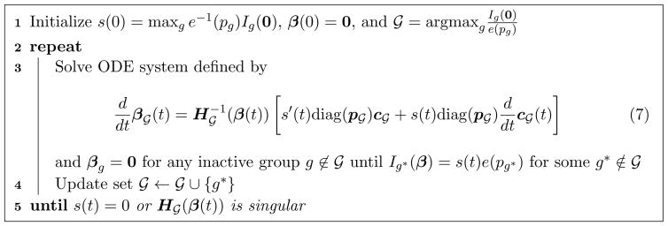
In this section we outline a strategy for extending ConvexLAR to incorporate group structure among predictors. Suppose predictors are divided into m groups with group size p_i, i = 1, …, m. Slightly abusing notation, we use g to represent both the g-th group and the index set of all predictors belonging to the g-th group. In a similar manner, we use 𝒢 to represent both the set of active groups and the index set of all predictors belonging to current active groups. For an arbitrary matrix H, H_ℐ,𝒥 denotes the sub-matrix of H with rows in ℐ and columns in 𝒥.

Group ConvexLAR can be devised based on the following considerations. (i) We need one way to gauge the aggregate “influence”, denoted by I_g(β), of a group g. For instance, we can use either the ℓ₂ norm or ℓ₁ norm of the sub-vector of the gradient corresponding to a group, i.e., $I_g(\mathit{\beta })={\Vert {\nabla }_{g}f(\mathit{\beta })\Vert }_2=\sqrt{{\sum }_{j\in g}{[{\nabla }_{j}f(\mathit{\beta })]}^2}$ or I_g(β) = ||∇_gf(β)||₁ = Σ_j∈g |∇_jf(β)|. Note that in principle any ℓ_p norm, p ≥ 1, can be used. (ii) For all groups in the active group set 𝒢, we use the function s(t) to control the common value of e(p_g)⁻¹I_g(β), g ∈ 𝒢, where p_g denotes the number of predictors in group g and e(p_g) is the effective size of g-th group. Common choices for e(p_g) are $\sqrt{p_g}$ or p_g. (iii) To make the ODE well defined, we need to assign the proportions of individual “influences” c_g(j) to each predictor j in group g. We require ||c_g||_p = 1 to satisfy the equation ||∇_gf(β)||_p = ||c_gI_g(β)||_p, where c_g is a column vector with c_g(j), j ∈ g, stacked together. These conditions imply the general group LAR identity

$${\nabla }_{j}f(\mathit{\beta })=c_g(j)I_g(\mathit{\beta })=c_g(j)e(p_g)s(t),j\in g,g\in \mathcal{G}.$$ (6)

Now the implicit function theorem yields the group LAR updating direction (7) in Algorithm 4. Here c_𝒢 is a column vector with c_g for g ∈ 𝒢 stacked together and p_𝒢 is a column vector with the corresponding effective group size e(p_g) for each predictor j in group g stacked together.

Algorithm 4.

A general scheme for Group ConvexLAR.

Specific choices of the group “influence” I_g(β), effective group size e(p_g), and individual “influence” c_g(j) lead to different updating directions. We specialize to the following three variants. The first has a close connection to the group lasso. The second and third recover two versions of group LAR algorithms developed in the literature.

1. GroupConvexLAR: We measure the group influence by I_g(β) = ||∇_gf(β)||₂, which is distributed to individual predictors within the group according to their effect size c_g(j) = −β_j/||β_g||₂. Let $e(p_g)=\sqrt{p_g}$ and assume 𝒢 = 𝒢₀ ∪ 𝒢₁, where 𝒢₀ = {g₀, …, g_a} denotes the set of active groups with ||β_g||₂ = 0 and 𝒢₁ = {g_a+1, …, g_a+b} denotes the set of active groups with ||β_g||₂ > 0.

   Theorem 2. For a strictly convex and twice differentiable loss function f(β), the LAR solution β(t) is continuous and differentiable at t within a segment.

   1. If 𝒢₀ is an empty set, the active solution vector β_𝒢(t) satisfies the differential equation

      $$\begin{array}{l}\frac{d}{dt}{\mathit{\beta }}_{\mathcal{G}}(t)={[{\mathit{H}}_{\mathcal{G}}(t)+\mathit{D}]}^{-1}{s}^{\prime }(t)\text{diag}({\mathit{p}}_{\mathcal{G}}){\mathit{c}}_{\mathcal{G}}\\ =\frac{s^{\prime }(t)}{s(t)}{[{\mathit{H}}_{\mathcal{G}}(t)+\mathit{D}]}^{-1}{\nabla }_{\mathcal{G}}f(\mathit{\beta }),\end{array}$$ (8)
      where D is the block diagonal matrix with blocks

      $$\frac{s(t)\sqrt{p_g}}{{\Vert {\mathit{\beta }}_g(t)\Vert }_2}\left({\mathit{I}}_{p_g}-\frac{1}{{\Vert {\mathit{\beta }}_g(t)\Vert }_2^2}{\mathit{\beta }}_g(t){\mathit{\beta }}_g^{\top }(t)\right),g\in \mathcal{G}.$$
   2. If 𝒢₀ is not empty, the solution vector β_gi for g_i ∈ 𝒢₀ satisfies

      $$\frac{d{\mathit{\beta }}_{g_i}(t)}{dt}=k_i{\nabla }_{g_i}f(\mathit{\beta }),$$ (9)
      and the constants k_i, i = 1, …, a, and updating direction for the groups in 𝒢₁ are jointly determined by

      $$\left(\begin{array}{c}{k}_1\\ ⋮\\ k_a\\ \frac{d}{dt}{\mathit{\beta }}_{{\mathcal{G}}_1}(t)\end{array}\right)=s(t){\left(\begin{array}{cc}\mathit{A}& {\mathit{B}}^{\top }\\ \mathit{B}& \mathit{C}\end{array}\right)}^{-1}\left(\begin{array}{c}{p}_{g_1}{s}^{\prime }(t)\\ ⋮\\ p_{g_a}{s}^{\prime }(t)\\ {\nabla }_{g_{a+1}}f(\mathit{\beta })/s^{\prime }(t)\\ ⋮\\ {\nabla }_{g_{a+b}}f(\mathit{\beta })/s^{\prime }(t)\end{array}\right),$$ (10)
      where A ∈ IR^a×a has entries a_ij = d_gif(β)H_gi,gj(β)∇_gj f(β), 1 ≤ i, j ≤ a,

      $$\mathit{B}=[\begin{array}{ccc}{\mathit{H}}_{{\mathcal{G}}_1,g_1}{\nabla }_{g_1}f(\mathit{\beta }),& \cdots ,& {\mathit{H}}_{{\mathcal{G}}_1,g_a}{\nabla }_{g_a}f(\mathit{\beta })\end{array}]\in {\text{IR}}^{{\sum }_{i=a+\mathit{1}}^{a+b}{p}_i\times a},$$
      and

      $$\mathit{C}={\mathit{H}}_{{\mathcal{G}}_1,{\mathcal{G}}_1}+{\mathit{D}}_{{\mathcal{G}}_1,{\mathcal{G}}_1}\in {\text{IR}}^{{\sum }_{i=a+\mathit{1}}^{a+b}{p}_i\times {\sum }_{i=a+\mathit{1}}^{a+b}{p}_i}.$$

      Note that, when 𝒢₀ is empty, (10) reduces to (8). The technical proof of Theorem 2 is delegated to the Appendix. Again the strict convexity assumption can be relaxed to the positive definiteness of H_𝒢(β(t)) along the path, which guarantees the non-singularity of the matrix involved in (10).

2. GroupConvexLAR-L1: We choose I_g(β) = ||∇_gf(β)||₁, e(p_g) = p_g and $c_g(j)=\frac{{\nabla }_{j}f(\mathit{\beta }(t_g))}{{\Vert {\nabla }_{g}f(\mathit{\beta }(t_g))\Vert }_1}$, where t_g is the time that the group g joins the active set 𝒢. Note that in this case c_g(j) is fixed for any j ∈ g once group g joins the active set. Therefore $\frac{d}{dt}{\mathit{c}}_{\mathcal{G}}(t)=\mathbf{0}$ and the group LAR direction (7) reduces to

   $$\frac{d}{dt}{\mathit{\beta }}_{\mathcal{G}}(t)=s^{\prime }(t){\mathit{H}}_{\mathcal{G}}{(\mathit{\beta })}^{-1}\text{diag}({\mathit{p}}_{\mathcal{G}}){\mathit{c}}_{\mathcal{G}}.$$ (11)

3. GroupConvexLAR-L2: With the choice I_g(β) = ||∇_gf(β)||₂, $e(p_g)=\sqrt{p_g}$ and $c_g(j)=\frac{{\nabla }_{j}f(\mathit{\beta }(t_g))}{{\Vert {\nabla }_{g}f(\mathit{\beta }(t_g))\Vert }_2}$, the ODE updating direction is same as (11) with the obvious substitute for c_𝒢 and p_𝒢.

   Note that, when all group sizes p_g are equal to 1,

   $$\frac{{\nabla }_{j}f(\mathit{\beta }(t_g))}{{\Vert {\nabla }_{g}f(\mathit{\beta }(t_g))\Vert }_2}=\frac{{\nabla }_{j}f(\mathit{\beta }(t_g))}{{\Vert {\nabla }_{g}f(\mathit{\beta }(t_g))\Vert }_1}=\frac{-{\beta }_j}{{\Vert {\mathit{\beta }}_g\Vert }_2}=sgn({\nabla }_{j}f(\mathit{\beta }))$$

   and $\frac{I_g(\mathit{\beta })}{e(p_g)}=\mid {\nabla }_{g}f(\mathit{\beta })\mid$ for all g. All three variants reduce to the ConvexLAR.

Connection with Previous Group LAR

Consider the variant GroupConvexLAR-L2 in the special case of least squares, i.e., $f(\mathit{\beta })={\Vert \mathit{y}-\mathit{X}\mathit{\beta }\Vert }_2^2/2$. In this case, both ${\mathit{H}}_{\mathcal{G}}(\mathit{\beta })={\mathit{X}}_{\mathcal{G}}^{\top }{\mathit{X}}_{\mathcal{G}}$ and c_𝒢(t) are constant within a segment. Thus, the group LAR updating direction (11) is constant within each segment, leading to a piecewise linear solution path with segment-wise slope

$$\frac{d}{dt}{\mathit{\beta }}_{\mathcal{G}}(t)=\frac{s^{\prime }(t)}{s(t)}{[{\mathit{X}}_{\mathcal{G}}^T{\mathit{X}}_{\mathcal{G}}]}^{-1}{\nabla }_{\mathcal{G}}f(\mathit{\beta }).$$

This recovers a version of group LAR proposed by Yuan and Lin (2006) for group selection in least squares. Park and Hastie (2006) argue that this version of group LAR tends to select a large group with only few of its component correlated with the response. To avoid this problem, they propose another version of group LAR by simply replacing the average squared correlation (Σ_j∈g[∇_jf(β)]²/p_g) with the average absolute correlation (Σ_j∈g |∇_jf(β)|/p_g), which is simply GroupConvexLAR-L1 specialized to least squares.

We emphasize that, for a general convex loss f, the solution paths by GroupConvexLARL1 and GroupConvexLAR-L2 are both piecewise smooth instead of piecewise linear and ODE solving is necessary.

3.3 Group ConvexLASSO Modification

We show next that a simple modification of the aforementioned first variant GroupConvexLAR yields the solution path of group lasso penalized problem min

$$\underset{\mathit{\beta }}{min}f(\mathit{\beta })+\lambda \sum _g\sqrt{p_g}{\Vert {\mathit{\beta }}_g\Vert }_2.$$

Its solution satisfies the following the Karush-Kuhn-Tucker (KKT) conditions

$${\nabla }_{g}f(\mathit{\beta })+\lambda \frac{\sqrt{p_g}}{{\Vert {\mathit{\beta }}_g\Vert }_2}{\mathit{\beta }}_g=0,{\mathit{\beta }}_g\ne \mathbf{0};$$ (12)

$${\Vert {\nabla }_{g}f(\mathit{\beta })\Vert }_2\le \lambda \sqrt{p_g},{\mathit{\beta }}_g=\mathbf{0}.$$ (13)

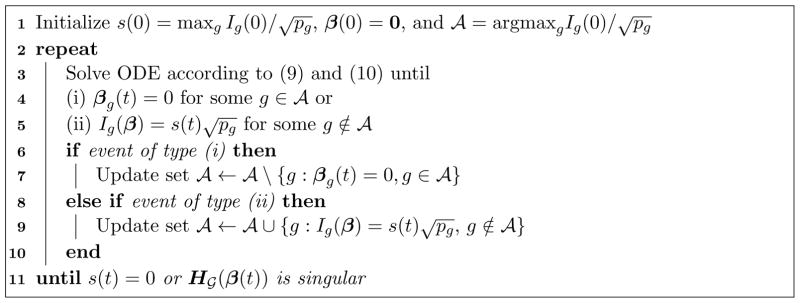
With the choice λ = s(t), the stationarity condition (12) coincides with the group LAR identity (6). This observation together with the above KKT conditions implies that the group lasso solution path moves along the same direction (8) of the GroupConvexLAR until either one of the following two types of event happens. The first type of event occurs when all predictors of an active group hit zero, denoted by event of type (i). The second type of event occurs when ||∇_gf(β)||₂ hits boundary $\lambda \sqrt{p_g}$, denoted by event of type (ii). Both types of event change the active set and redefine the direction. The second type of event is already considered in the GroupConvexLAR algorithm. Thus a simple modification of GroupConvexLAR by tracking the first type of event leads to the group lasso solution path. This modification is summarized in Algorithm 5. This exact path following algorithm for the group lasso penalized convex loss seems new. On a side note, there is no obvious connection between GroupConvexLAR-L1, L2 and group lasso.

Algorithm 5.

Group ConvexLASSO.

4 Examples

We illustrate ConvexLAR and its extensions on various statistical problems. To demonstrate the efficiency of the proposed algorithm, we report the running times of all numeric examples on i7 Core 2.93GHz, 8G RAM averaged over 50 independent runs.

4.1 Recurrent event data

Suppose that we have n independent subjects in a recurrent event study. For each subject i, N_i(t) denotes the number of events that occur over the interval (0, t] and x_i ∈ IR^p is the corresponding covariate vector. Assume that given x_i, the counting process {N_i(t)} is a non-homogeneous Poisson process with mean function

$${\mu }_i(t)=\mathrm{E}\{N_i(t)\mid {\mathit{x}}_i\}={\mu }_0(t)exp({\mathit{x}}_i^{\top }\mathit{\beta })$$ (14)

for some unknown continuous baseline mean function μ₀(t) and unknown parameters β ∈ IR^p. See Tong et al. (2009b) for a detailed introduction to recurrent event data.

As typical in survival study, each subject is subject to potential censoring. Let C_i denote the follow-up or dropout time for subject i and Ñ_i(t) = N_i(min(t,C_i)) be a point process for subject i’s observed process. The observed data are summarized as {(Ñ_i(t),C_i, x_i), i = 1, 2,⋯, n, 0 ≤ t ≤ T}, where the constant T denotes the maximum potential follow-up time. The log-partial likelihood function based on model (14) is given by

$$\ell (\mathit{\beta })=\frac{1}{n}\sum _{i=1}^n{\int }_0^{\top }\left[{\mathit{x}}_i^{\top }\mathit{\beta }-ln\left\{\sum _{j=1}^n{Y}_j(t)exp({\mathit{x}}_j^{\top }\mathit{\beta })\right\}\right]d{\stackrel{\sim }{N}}_i(t).$$ (15)

Under mild regularity conditions, the log-partial likelihood ℓ(β) is strictly concave in β. Thus in this example, our objective function is chosen to be f(β) = −ℓ(β). The first two derivatives of f(β) with respect to β are

$$\begin{array}{ll}\hfill \nabla f(\mathit{\beta })& =-\frac{1}{n}\sum _{i=1}^n{\int }_0^{\top }\left[{\mathit{x}}_i-\frac{{\sum }_{j=1}^n{Y}_j(t)exp({\mathit{x}}_j^{\top }\mathit{\beta }){\mathit{x}}_j}{{\sum }_{j=1}^n{Y}_j(t)exp({\mathit{x}}_j^{\top }\mathit{\beta })}\right]d{\stackrel{\sim }{N}}_i(t),\\ \hfill d^{2}f(\mathit{\beta })& =\frac{1}{n}\sum _{i=1}^n{\int }_0^{\top }\left[\frac{{\sum }_{j=1}^n{Y}_j(t)exp({\mathit{x}}_j^{\top }\mathit{\beta }){\mathit{x}}_j{\mathit{x}}_j^{\top }}{{\sum }_{j=1}^n{Y}_j(t)exp({\mathit{x}}_j^{\top }\mathit{\beta })}-\frac{\left({\sum }_{j=1}^n{Y}_j(t)exp({\mathit{x}}_j^{\top }\mathit{\beta }){\mathit{x}}_j\right){\left({\sum }_{j=1}^n{Y}_j(t)exp({\mathit{x}}_j^{\top }\mathit{\beta }){\mathit{x}}_j\right)}^{\top }}{{\left({\sum }_{j=1}^n{Y}_j(t)exp({\mathit{x}}_j^{\top }\mathit{\beta })\right)}^2}\right]d{\stackrel{\sim }{N}}_i(t).\end{array}$$

Tong et al. (2009b) studied a Chronic Granulomatous Disease (CGD) data which were collected from a multicenter placebo-controlled randomized trial of gamma inferon with chronic granulotomous disease. There were 128 patients randomized to two groups, gamma interferon group (n₁ = 63) and placebo group (n₂ = 65). For each patient the times from the beginning of the study to initial and any recurrent serious infections are available. Eleven covariates are considered: 1. trtmt=treatment (Yes/No), 2. inherit=pattern of inheritance (autosomal/recessive), 3. age, 4. height, 5. weight, 6. cortico=use of corticosteroids (Yes/No), 7. prophy=use of prophylactic antibiotics (Yes/No), 8. gender=female, 9. hosp1=hosp. (category: US/other), 10. hosp2=hosp. (category: Europe-Amsterdam), and 11. hosp3=hosp. (category: Europe-other). We standardize all continuous covariates (age, height and weight) to have mean 0 and unit length. Furthermore, we also include the six quadratic and interaction terms between three continuous covariates. They are: 12. age×age, 13. height×height, 14. weight×weight, 15. age×height, 16. age×weight, 17. height×weight.

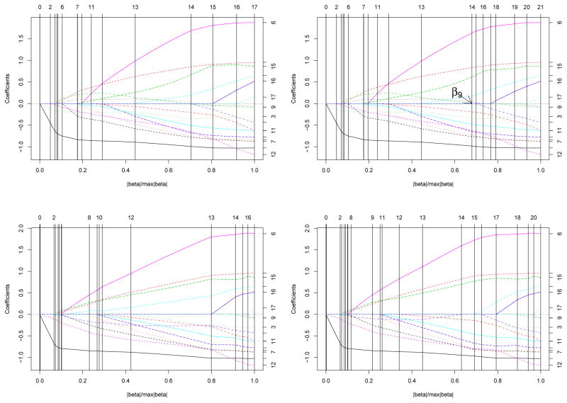
Figure 1 shows the solution paths from different algorithms. Here the numbers on the right hand side indicate which variable each path corresponds to. In all plots, the x-axes are in the units of ||β(t)||₁/max_t ||β(t)||₁ and vertical lines mark the event times for easy comparison between various solution paths. Top row of Figure 1 displays the ConvexLAR (top left panel) and ConvexLASSO (top right panel) solution paths for the CGD data. They are qualitatively different. For instance, in the ConvexLASSO path, β₉ hits zero and then escapes active set at Step 14. In addition we also apply the weighted CovexLAR and ConvexLASSO algorithms with weights set at the maximum likelihood estimator of equation (15). They differ significantly from the unweighted ones. The running times are 4.84, 5.60, 5.34 and 6.37 seconds for the ConvexLAR, ConvexLASSO, weighted ConvexLAR and weighted ConvexLASSO solution paths, respectively.

Figure 1.

Recurrent event example (CGD data). Top left: ConvexLAR; Top right: ConvexLASSO; Bottom left: weighted ConvexLAR; Bottom right: weighted ConvexLASSO.

4.2 Panel Count Data

In the above recurrent event example, we assume that the exact time of each event, if not censored, is observed. Unfortunately this is not the case in many studies. The model for panel count data (Sun and Wei, 2000; Tong et al., 2009a) provides a remedy.

Let T_i1 < T_i2 < ⋯ < T_imi be the potential observation times on process N_i(t) and $H_i(t)={\sum }_{j=1}^{m_i}I(T_{ij}\le t)$ denote the observation process. Let H̃_i(t) = H(min(t, C_i)) be the actual observation times after censoring. Then the observed data for panel count model are

$$\{(N_i(t)d{\stackrel{\sim }{H}}_i(t),{\stackrel{\sim }{H}}_i(t),C_i,{\mathit{x}}_i^{\top }),i=1,\dots ,n,0\le t\le T\}.$$

When H_i and C_i are mutually independent and also independent of N_i and x_i, Sun and Wei (2000) propose to estimate regression parameters by solving the following estimation equation

$$W(\mathit{\beta })=\sum _{i=1}^n{\overline{N}}_i{e}^{-{\mathit{x}}_i^{\top }\mathit{\beta }}{\mathit{x}}_i=\mathbf{0},$$

where ${\overline{N}}_i={\int }_0^{\top }{N}_i(t)d{\stackrel{\sim }{H}}_i(t)$. ConvexLAR and its extensions can be applied directly to the influence function

$$-W(\mathit{\beta })=\sum _{i=1}^n{\overline{N}}_i{e}^{-{\mathit{x}}_i^{\top }\mathit{\beta }}{\mathit{x}}_i$$

which has a positive definite derivative

$$-DW(\mathit{\beta })=\sum _{i=1}^n{\overline{N}}_i{e}^{-{\mathit{x}}_i^{\top }\mathit{\beta }}{\mathit{x}}_i{\mathit{x}}_i^{\top }.$$

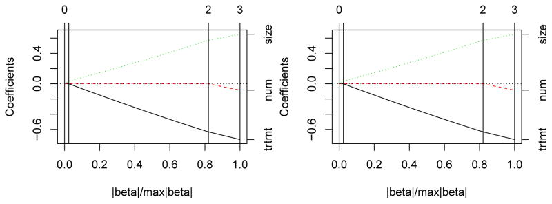
We illustrate with the bladder tumor recurrence data considered in Sun and Wei (2000). A total of 85 bladder tumor patients were randomized into two treatment groups, i.e., placebo group and thiotepa treatment group. Most patients visited the hospital several times to have their recurrent tumors removed. The number of new tumors discovered at each visit was recorded and removed after each visit. The binary treatment (trtmt) is one of our explanatory covariates. Furthermore, we consider two additional important baseline covariates, the number of initial tumors (num) and the size of the largest initial tumor (size). All covariates are centered around zero and scaled to have unit length. Figure 2 shows the ConvexLAR and ConvexLASSO solution paths for this example. The two solution paths are identical in this particular example as no active predictors return to zero along the path. The running times are 0.04 and 0.05 seconds for the ConvexLAR and ConvexLASSO solution paths, respectively.

Figure 2.

ConvexLAR and ConvexLASSO solution paths for the panel count data (bladder) example.

4.3 Ada-Boost

Ada-Boost is considered one of the best off-the-shelf classification methods (Hastie et al., 2009). In binary classification, we are given a training data set {(x_i, y_i} : i = 1, ⋯, n} with x_i ∈ IR^p and y_i ∈{−1, +1}. The goal is to estimate a function f(x) whose sign will be used as the classification rule. For simplicity we consider the linear classification, in which f(x) = β₀ + x^⊤β. The Ada-Boost estimates parameters by solving

$$\underset{{\beta }_0,\mathit{\beta }}{min}\sum _{i=1}^n{e}^{-y_i({\beta }_0+{\mathit{x}}_i^{\top }\mathit{\beta })},$$ (16)

which is strictly convex and thus amenable to our ConvexLAR algorithm. Denote 𝒟 = {i : y_i = −1}. Define the marginal minimizer of β₀ as a function of β

$${\mathit{\beta }}_0(\mathit{\beta })={\text{argmin}}_{{\mathit{\beta }}_0}f({\mathit{\beta }}_0,\mathit{\beta })=\frac{1}{2}log\left\{\frac{{\sum }_{i\in {\mathcal{D}}^c}{e}^{-{\mathit{x}}_i^{\top }\mathit{\beta }}}{{\sum }_{i\in \mathcal{D}}{e}^{{\mathit{x}}_i^{\top }\mathit{\beta }}}\right\}.$$ (17)

Thus the first two derivatives of f(β) with respect to β are

$$\begin{array}{l}\nabla f(\mathit{\beta })=\left(\frac{\partial {\beta }_0}{\partial \mathit{\beta }}\right)\left[e^{{\beta }_0}\sum _{\mathcal{D}}{e}^{{\mathit{x}}_i^{\top }\mathit{\beta }}-e^{-{\beta }_0}\sum _{{\mathcal{D}}^c}{e}^{-{\mathit{x}}_i^{\top }\mathit{\beta }}\right]+\left[e^{{\beta }_0}\sum _{\mathcal{D}}{e}^{{\mathit{x}}_i^{\top }\mathit{\beta }}{\mathit{x}}_i-e^{-{\beta }_0}\sum _{{\mathcal{D}}^c}{e}^{-{\mathit{x}}_i^{\top }\mathit{\beta }}{\mathit{x}}_i\right],\\ d^{2}f(\mathit{\beta })=\left(\frac{{\partial }^2{\beta }_0}{\partial \mathit{\beta }\partial {\mathit{\beta }}^{\top }}\right)\left[e^{{\beta }_0}\sum _{\mathcal{D}}{e}^{{\mathit{x}}_i^{\top }\mathit{\beta }}-e^{-{\beta }_0}\sum _{{\mathcal{D}}^c}{e}^{-{\mathit{x}}_i^{\top }\mathit{\beta }}\right]\\ +\left(\frac{\partial {\beta }_0}{\partial \mathit{\beta }}\right){\left(\frac{\partial {\beta }_0}{\partial \mathit{\beta }}\right)}^{\top }\left[e^{{\beta }_0}\sum _{\mathcal{D}}{e}^{{\mathit{x}}_i^{\top }\mathit{\beta }}+e^{-{\beta }_0}\sum _{{\mathcal{D}}^c}{e}^{-{\mathit{x}}_i^{\top }\mathit{\beta }}\right]\\ +\left(\frac{\partial {\beta }_0}{\partial \mathit{\beta }}\right){\left[e^{{\beta }_0}\sum _{\mathcal{D}}{e}^{{\mathit{x}}_i^{\top }\mathit{\beta }}{\mathit{x}}_i+e^{-{\beta }_0}\sum _{{\mathcal{D}}^c}{e}^{-{\mathit{x}}_i^{\top }\mathit{\beta }}{\mathit{x}}_i\right]}^{\top }\\ +\left[e^{{\beta }_0}\sum _{\mathcal{D}}{e}^{{\mathit{x}}_i^{\top }\mathit{\beta }}{\mathit{x}}_i+e^{-{\beta }_0}\sum _{{\mathcal{D}}^c}{e}^{-{\mathit{x}}_i^{\top }\mathit{\beta }}{\mathit{x}}_i\right]{\left(\frac{\partial {\beta }_0}{\partial \mathit{\beta }}\right)}^{\top }\\ +\left[e^{{\beta }_0}\sum _{\mathcal{D}}{e}^{{\mathit{x}}_i^{\top }\mathit{\beta }}{\mathit{x}}_i{\mathit{x}}_i^{\top }+e^{-{\beta }_0}\sum _{{\mathcal{D}}^c}{e}^{-{\mathit{x}}_i^{\top }\mathit{\beta }}{\mathit{x}}_i{\mathit{x}}_i^{\top }\right],\end{array}$$

where

$$\begin{array}{l}\frac{\partial {\beta }_0(\mathit{\beta })}{\partial \mathit{\beta }}=-\frac{1}{2}\left\{\frac{{\sum }_{{\mathcal{D}}^c}{e}^{-{\mathit{x}}_i^{\top }\mathit{\beta }}{\mathit{x}}_i}{{\sum }_{{\mathcal{D}}^c}{e}^{-{\mathit{x}}_i^{\top }\mathit{\beta }}}+\frac{{\sum }_{\mathcal{D}}{e}^{{\mathit{x}}_i^{\top }\mathit{\beta }}{\mathit{x}}_i}{{\sum }_{\mathcal{D}}{e}^{{\mathit{x}}_i^{\top }\mathit{\beta }}}\right\},\\ \frac{{\partial }^2{\beta }_0(\mathit{\beta })}{\partial \mathit{\beta }\partial {\mathit{\beta }}^{\top }}=\frac{1}{2}\left\{\frac{\left({\sum }_{{\mathcal{D}}^c}{e}^{-{\mathit{x}}_i^{\top }\mathit{\beta }}{\mathit{x}}_i{\mathit{x}}_i^{\top }\right)\left({\sum }_{{\mathcal{D}}^c}{e}^{-{\mathit{x}}_i^{\top }\mathit{\beta }}\right)-\left({\sum }_{{\mathcal{D}}^c}{e}^{-{\mathit{x}}_i^{\top }\mathit{\beta }}{\mathit{x}}_i\right){\left({\sum }_{{\mathcal{D}}^c}{e}^{-{\mathit{x}}_i^{\top }\mathit{\beta }}{\mathit{x}}_i\right)}^{\top }}{{\left({\sum }_{{\mathcal{D}}^c}{e}^{-{\mathit{x}}_i^{\top }\mathit{\beta }}\right)}^2}\right\}\\ -\frac{1}{2}\left\{\frac{\left({\sum }_{\mathcal{D}}{e}^{{\mathit{x}}_i^{\top }\mathit{\beta }}{\mathit{x}}_i{\mathit{x}}_i^{\top }\right)\left({\sum }_{\mathcal{D}}{e}^{{\mathit{x}}_i^{\top }\mathit{\beta }}\right)-\left({\sum }_{\mathcal{D}}{e}^{{\mathit{x}}_i^{\top }\mathit{\beta }}{\mathit{x}}_i\right){\left({\sum }_{\mathcal{D}}{e}^{{\mathit{x}}_i^{\top }\mathit{\beta }}{\mathit{x}}_i\right)}^{\top }}{{\left({\sum }_{\mathcal{D}}{e}^{{\mathit{x}}_i^{\top }\mathit{\beta }}\right)}^2}\right\}.\end{array}$$

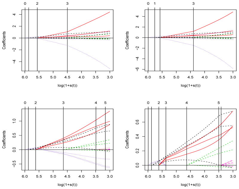
The Wisconsin Diagnostic Breast Cancer (WDBC) data (Frank and Asuncion, 2010) are collected on n = 569 patients from digitized images of a fine needle aspirate (FNA) of their breast mass. The number of predictors is p = 10. The mean, standard error, and “worst” or largest (mean of the three largest values) of these predictors were computed for each patient, resulting in 30 features forming 10 groups each of size 3. The response is binary in that each patient is diagnosed either as malignant (Y = 1) or benign (Y = −1). Each predictor variable is standardized to have mean zero and variance one. Figure 3 displays the group ConvexLARs solution paths for this example. The x-axis is log(1+s(t)), where s(t) is the same as the λ in group ConvexLASSO. To have a clear view, only the solution paths where log(1 + s(t)) > 3 are plotted. GroupConvexLAR-L2 and GroupConvexLAR-L1 appear quite different from GroupConvexLAR with larger max_i∈𝒢 |β_i(t)| across the same level of s(t). Bottom row of Figure 3 displays the GroupConvexLAR and Group ConvexLASSO solution paths, which are fundamentally different for the WDBC data. The third group (displayed with dotted line) is the first active one and then stay active along the whole GroupConvexLAR solution path. In contrast, the same group hits zero in the event 3 of the Group ConvexLASSO solution path and escapes the active set thereafter. The running times are 1.53, 1.58, 1.49 and 2.13 seconds for the GroupConvexLAR-L2, GroupConvexLAR-L1, GroupConvexLAR and GroupConvexLASSO solution paths, respectively.

Figure 3.

Group LARs solution paths for the Ada-Boost data (WDBC) example. Top left: GroupConvexLAR-L2; Top right: GroupConvexLAR-L1; Bottom left: GroupConvexLAR; Bottom right: Group ConvexLASSO.

4.4 Gaussian graphical model

Our fourth example concerns the LAR for Gaussian graphical model. Assume we have iid observations x₁, x₂, ⋯, x_n ∈ IR^p from N(0, Σ). Denote the sample variance covariance matrix by $\widehat{\mathbf{\sum }}=\frac{1}{n}{\sum }_{i=1}^n{\mathit{x}}_i{\mathit{x}}_i^{\top }$ and precision matrix by Ω = Σ^−1. Then the negative likelihood for Ω is given by −ℓ(Ω) = −log detΩ + tr(Σ̂Ω), which is convex. Let ω_ij denote the (i, j)-element of Ω. w_ij = 0, i ≠ j, implies the conditional independence between variables i and j. We partition the parameters into the sets Ω₀ = (ω₁₁, ω₂₂, ⋯, ω_pp)^⊤ ∈ IR^p and Ω₁ = (ω₁₂, ω₁₃, ⋯, ω_(p−1)p)^⊤ ∈ IR^p(p−1)/2. Only those in Ω₁ are subject to regularization. We may rewrite the negative loglikelihood as −ℓ(Ω₀,Ω₁). For every fixed Ω₁, we define Ω₀(Ω₁) = argmin_Ω0 − ℓ(Ω₀, Ω₁). With these notations, we have f(Ω₁) = −ℓ(Ω₀(Ω₁), Ω₁).

To derive the LAR solution path, we need the first two derivatives of the objective function

$$f({\mathbf{\Omega }}_0,{\mathbf{\Omega }}_1)=-logdet\mathbf{\Omega }({\mathbf{\Omega }}_0,{\mathbf{\Omega }}_1)+\text{tr}(\widehat{\mathbf{\sum }}\mathbf{\Omega }({\mathbf{\Omega }}_0,{\mathbf{\Omega }}_1)),$$

where Ω₀ is implicitly determined by Ω₁. We first show how to determine Ω₀ given Ω₁. Setting partial derivative of f with respect to Ω₀

$$D_{{\mathbf{\Omega }}_0}f({\mathbf{\Omega }}_0,{\mathbf{\Omega }}_1)=D_{{\mathbf{\Omega }}_0}f(\mathbf{\Omega })D\mathbf{\Omega }({\mathbf{\Omega }}_0)=-{(\text{vec}{\mathbf{\Omega }}^{-1})}^{\top }D\mathbf{\Omega }({\mathbf{\Omega }}_0)+{(\text{vec}\widehat{\mathbf{\sum }})}^{\top }D\mathbf{\Omega }({\mathbf{\Omega }}_0)$$

to 0 gives the stationarity condition

$$\text{diag}({\mathbf{\Omega }}^{-1}({\mathbf{\Omega }}_0,{\mathbf{\Omega }}_1))={({\widehat{\sigma }}_{11},\dots ,{\widehat{\sigma }}_{pp})}^{\top }.$$

In other words, given Ω₁, we need to choose Ω₀ such that the diagonal entries of Ω⁻¹ match those of Σ̂. In practice, Newton’s iteration

$${\omega }_0^{(t+1)}={\omega }_0^{(t)}+{\{{[D\mathbf{\Omega }({\mathbf{\Omega }}_0)]}^{\top }[{\mathbf{\Omega }}^{-1}\otimes {\mathbf{\Omega }}^{-1}][D\mathbf{\Omega }({\mathbf{\Omega }}_0)]\}}^{-1}[\text{diag}({\mathbf{\Omega }}^{-1}-\widehat{\mathbf{\sum }})]$$

can be applied to solve for Ω₀ given Ω₁. We denote this mapping by Ω₀(Ω₁). The gradient DΩ₀(Ω₁) ∈ ℝ^{p×p(p−1)/2} will be of use later and is obtained through the implicit function theorem

$$D{\mathbf{\Omega }}_0({\mathbf{\Omega }}_1)=-{\{{[D\mathbf{\Omega }({\mathbf{\Omega }}_0)]}^{\top }({\mathbf{\Omega }}^{-1}\otimes {\mathbf{\Omega }}^{-1})[D\mathrm{\Omega }({\mathbf{\Omega }}_0)]\}}^{-1}{[D\mathbf{\Omega }({\mathbf{\Omega }}_0)]}^{\top }({\mathbf{\Omega }}^{-1}\otimes {\mathbf{\Omega }}^{-1})[D\mathrm{\Omega }({\mathbf{\Omega }}_1)].$$ (18)

Now the first derivative of objective function f with respect to Ω₁ is

$$D_{{\mathbf{\Omega }}_1}f({\mathbf{\Omega }}_0({\mathbf{\Omega }}_1),{\mathbf{\Omega }}_1)=D_{{\mathbf{\Omega }}_1}f({\mathbf{\Omega }}_0,{\mathbf{\Omega }}_1)+D_{{\mathbf{\Omega }}_0}f({\mathbf{\Omega }}_0,{\mathbf{\Omega }}_1)D{\mathbf{\Omega }}_0({\mathbf{\Omega }}_1)$$

but the second term vanishes because D_Ω0 f(Ω₀, Ω₁) = 0. Hence

$$D_{{\mathbf{\Omega }}_1}f({\mathbf{\Omega }}_0({\mathbf{\Omega }}_1),{\mathbf{\Omega }}_1)=Df(\mathbf{\Omega })D\mathbf{\Omega }({\mathbf{\Omega }}_1)={(-\text{vec}{\mathbf{\Omega }}^{-1}+\text{vec}\widehat{\mathbf{\sum }})}^{\top }D\mathbf{\Omega }({\mathbf{\Omega }}_1).$$

In words, given current Ω₁, calculate Ω⁻¹ at optimal Ω₀; then the off-diagonal entries of 2(Σ̂ − Ω⁻¹) form the gradient of f in terms of Ω₁. For the Hessian,

$$\begin{array}{l}Hf({\mathbf{\Omega }}_1)=D_{{\mathbf{\Omega }}_1}{[D_{{\mathbf{\Omega }}_1}f({\mathbf{\Omega }}_0({\mathbf{\Omega }}_1),{\mathbf{\Omega }}_1)]}^{\top }\\ =D_{{\mathbf{\Omega }}_1}[D\mathbf{\Omega }{({\mathbf{\Omega }}_1)}^{\top }(-\text{vec}{\mathbf{\Omega }}^{-1}+\text{vec}\widehat{\mathbf{\sum }})]\\ =-D_{{\mathbf{\Omega }}_1}[D\mathbf{\Omega }{({\omega }_1)}^{\top }(\text{vec}{\mathbf{\Omega }}^{-1})]\\ =-{[D\mathbf{\Omega }({\omega }_1)]}^{\top }({\mathbf{\Omega }}^{-1}\otimes {\mathbf{\Omega }}^{-1})[D\mathbf{\Omega }({\mathbf{\Omega }}_1)+D\mathbf{\Omega }({\mathbf{\Omega }}_0)D{\mathbf{\Omega }}_0({\mathbf{\Omega }}_1)].\end{array}$$ (19)

Now substitute DΩ₀(Ω₁) by the expression (18).

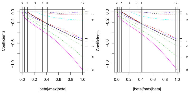
We illustrate our algorithm by two examples. The first data set contains 88 students’ scores on five math courses - mechanics, vector, algebra, analysis and statistics. See Table 1.2.1 of Mardia et al. (1979) for more details. Figure 4 displays the ConvexLAR and ConvexLASSO solution paths. The most important three edges are analysis-algebra, statisticsalgebra, and algebra-vector by lasso regularization. The ConvexLAR and ConvexLASSO solution paths coincide in this example. The running times are 0.28 and 0.37 seconds for the ConvexLAR and ConvexLASSO solution paths, respectively.

Figure 4.

ConvexLAR and ConvexLASSO solution paths for the graphical model (math score) example.

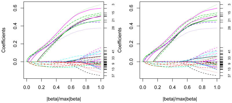
Our second example concerns a simulated data set with p = 10 and n = 200 and illustrates a case where ConvexLAR and ConvexLASSO yield different paths. The true precision matrix Ω = (ω_ij) has entries ω_ii = 1, ω_i,i−1 = 0.5, ω_i,i+1 = 0.5, and ω_ij = 0 for |i − j| > 1. There are 45 non-diagonal free parameters. Figure 5 displays the ConvexLAR and ConvexLASSO solution paths. The solution paths appear different. The running times are 1.63 and 2.62 seconds for the ConvexLAR and ConvexLASSO solution paths, respectively.

Figure 5.

ConvexLAR and ConvexLASSO solution paths for the graphical model example with the simulated data.

5 Discussion

Variable selection has become an essential tool for modern data analysis. So far penalization method such as lasso has been the dominant regularization technique and extended to handle increasingly more applications. In contrast, the original LAR (Efron et al., 2004) has received much less generalizations despite its popularity. In this expository article, we show that the simple geometric idea in LAR can be naturally extended to various situations such as convex loss, group structures in predictors, and data adaptive regularizations. The classical score function plays an essential role throughout the development. The original “least angle” idea translates to the equality of contributions by the active predictors to the score function. In our understanding, this is the fundamental idea in LAR and underpins the various extensions presented in this article.

This illustrative article is meant to whet readers’ appetites not satiate them. Much is left undone. For instance, in principle it is the estimation equation that LAR operates on. Therefore LAR naturally applies many statistical methods without a natural loss function such as generalized estimation equation (GEE), as hinted in the panel count data in Section 4. In this article we focus on LAR algorithmic development and forego the theoretical treatment. There has been intensive study of the asymptotic properties of regularized estimates by penalty methods in recent years. Same study for ConvexLAR is worth pursuing. Especially those that might shed light on the difference between the two regularization methods are much desired.

Appendix

Proof of Theorem 1

The LAR fundamental identity (1) for active predictors dictates the vector equation

$$k({\mathit{\beta }}_{\mathcal{A}},t)={\nabla }_{\mathcal{A}}f(\mathit{\beta })-\text{sgn}({\nabla }_{\mathcal{A}}f(\mathit{\beta }))s(t)=\mathbf{0}.$$

To solve for β_𝒜 in terms of t, we apply the implicit function theorem (Lange, 2004). This requires calculating the differential of k with respect to the dependent variables β_𝒜 and the independent variable t

$$\begin{array}{ll}\hfill {\partial }_{{\mathit{\beta }}_{\mathcal{A}}}k({\mathit{\beta }}_{\mathcal{A}},t)& ={\mathit{H}}_{\mathcal{A}}(\mathit{\beta },t)\\ \hfill {\partial }_{t}k({\mathit{\beta }}_{\mathcal{A}},t)& =-s^{\prime }(t)\text{sgn}({\nabla }_{\mathcal{A}}f(\mathit{\beta })).\end{array}$$

Given the non-singularity of H_𝒜(β, t), the implicit function theorem applies and shows the continuity and differentiability of β_𝒜(t) at t. Furthermore, it supplies the derivative (2).

Derivation of GroupConvexLAR directions (8), (9) and (10)

We use 𝒢₀ to denote the set of active groups that equal to 0. Let 𝒢₁ = 𝒢 − 𝒢₀, where 𝒢 denotes the set of all active groups. We slightly abuse notation by letting 𝒢₀, 𝒢₁ and 𝒢 to denote both the sets of groups and the set of all predictors belonging to the corresponding groups. Obviously, 𝒢₀, 𝒢₁ and 𝒢 depend on the time index t.

Derivation of updating direction hinges upon the LAR identity (6), which we rewrite here for convenience

$${\nabla }_{g}f(\mathit{\beta })+\sqrt{p_g}s(t)\frac{{\mathit{\beta }}_g}{{\Vert {\mathit{\beta }}_g\Vert }_2}={\mathbf{0}}_{p_g},g\in \mathcal{G}.$$ (20)

1. When 𝒢₀ is empty, differentiating the vector equation (20) with respect to t via chain rule gives

   $$\left[{\mathit{H}}_{g,\mathcal{G}}(\mathit{\beta })+\sqrt{p_g}\frac{s(t)}{{\Vert {\mathit{\beta }}_g\Vert }_2}\left({\mathit{I}}_{p_g}-\frac{{\mathit{\beta }}_g{\mathit{\beta }}_g^{\top }}{{\Vert {\mathit{\beta }}_g\Vert }_2^2}\right)D_{{\mathit{\beta }}_{\mathcal{G}}}{\mathit{\beta }}_g\right]\frac{d{\mathit{\beta }}_{\mathcal{G}}(t)}{dt}+\sqrt{p_g}{s}^{\prime }(t)\frac{{\mathit{\beta }}_g}{\Vert {\mathit{\beta }}_g\Vert }={\mathbf{0}}_{p_g},$$ (21)
   where $D_{{\mathit{\beta }}_{\mathcal{G}}}{\mathit{\beta }}_g=(\mathbf{0},{\mathit{I}}_{p_g},\mathbf{0})\in {\text{IR}}^{p_g\times {\sum }_{i=1}^{a+b}{g}_i}$. Combining all |𝒢| vector equations and rearranging yields the LAR updating direction

   $$\frac{d}{dt}{\mathit{\beta }}_{\mathcal{G}}(t)=-{[{\mathit{H}}_{\mathcal{G}}(t)+\mathit{D}]}^{-1}\sqrt{p_g}{s}^{\prime }(t)\frac{{\mathit{\beta }}_g}{\Vert {\mathit{\beta }}_g\Vert }=\frac{s^{\prime }(t)}{s(t)}{[{\mathit{H}}_{\mathcal{G}}(t)+\mathit{D}]}^{-1}{\nabla }_{\mathcal{G}}f(\mathit{\beta }),$$ (22)
   where D is the block diagonal matrix with blocks

   $$\sqrt{p_g}\frac{s(t)}{{\Vert {\mathit{\beta }}_g\Vert }_2}\left({\mathit{I}}_{p_g}-\frac{{\mathit{\beta }}_g{\mathit{\beta }}_g^{\top }}{{\Vert {\mathit{\beta }}_g\Vert }_2^2}\right),g\in \mathcal{G}.$$
2. When 𝒢₀ not empty, we assume that 𝒢₀ contains a groups, g₁, …, g_a, and 𝒢₁ contains b groups, g_a+1, …, g_a+b. By rearranging the order of groups, we have ${\mathit{\beta }}_{\mathcal{G}}^{\top }=({\mathit{\beta }}_{{\mathcal{G}}_0}^{\top },{\mathit{\beta }}_{{\mathcal{G}}_1}^{\top })$, where ${\mathit{\beta }}_{{\mathcal{G}}_0}^{\top }=({\mathit{\beta }}_{g_1}^{\top },{\mathit{\beta }}_{g_2}^{\top },\dots ,{\mathit{\beta }}_{g_a}^{\top })$ and ${\mathit{\beta }}_{{\mathcal{G}}_1}^{\top }=({\mathit{\beta }}_{g_{a+1}}^{\top },{\mathit{\beta }}_{g_{a+2}}^{\top },\dots ,{\mathit{\beta }}_{g_{a+b}}^{\top })$. For any group g ∈ 𝒢₁, i.e., ||β_g||₂ ≠ 0, the vector equation (21) still holds which gives

   $$\left[{\mathit{H}}_{g,\mathcal{G}}(\mathit{\beta })+\frac{\sqrt{p_g}s(t)}{{\Vert {\mathit{\beta }}_g\Vert }_2}\left({\mathit{I}}_{p_g}-\frac{{\mathit{\beta }}_g{\mathit{\beta }}_g^{\top }}{{\Vert {\mathit{\beta }}_g\Vert }_2}\right)D_{{\mathit{\beta }}_{\mathcal{G}}}{\mathit{\beta }}_g\right]\frac{d{\beta }_{\mathcal{G}}(t)}{dt}=\frac{s(t)}{s^{\prime }(t)}{\nabla }_{g}f(\mathit{\beta }).$$ (23)
   Unfortunately it does not hold for any g ∈ 𝒢₀ due to the singularity ||β_g||₂ = 0. First we show that the updating direction of such groups is proportional to their gradient sub-vectors. By the LAR identity (20) and the fact β_g(t) = 0_pg,

   $$\frac{[{\mathit{\beta }}_g(t+\delta t)-{\mathit{\beta }}_g(t)]/\delta t}{{\Vert [{\mathit{\beta }}_g(t+\delta t)-{\mathit{\beta }}_g(t)]/\delta t\Vert }_2}=-\frac{1}{\sqrt{p_g}s(t+\delta t)}{\nabla }_{g}f(\mathit{\beta }(t+\delta t))$$
   for all δt > 0. Taking limit δt ↓ 0 yields

   $$\frac{d{\mathit{\beta }}_g(t)}{dt}=k_g{\nabla }_{g}f(\mathit{\beta }),$$ (24)

   where k_g are the constants to be determined.

Equating the norms of the two summand vectors in the LAR identity (20) shows ${\Vert {\nabla }_{g}f(\mathit{\beta })\Vert }_2^2=p_g{s}^2(t)$. Differentiating both sides of this identity with respect to t via chain rule gives

$$d_{g}f(\mathit{\beta }){\mathit{H}}_{g,\mathcal{G}}(\mathit{\beta })\frac{d{\mathit{\beta }}_{\mathcal{G}}(t)}{dt}=p_{g}s(t)s^{\prime }(t)$$ (25)

for any g ∈ 𝒢₀. Now substituting (24) into the equations (23) and (25), we obtain

$$\left(\begin{array}{cc}\mathit{A}& {\mathit{B}}^{\top }\\ \mathit{B}& \mathit{C}\end{array}\right)\left(\begin{array}{c}{k}_1\\ ⋮\\ k_a\\ \frac{d}{dt}{\mathit{\beta }}_{{\mathcal{G}}_1}(t)\end{array}\right)=\left(\begin{array}{c}{p}_{g_1}{s}^{\prime }(t)\\ ⋮\\ p_{g_a}{s}^{\prime }(t)\\ {\nabla }_{g_{a+1}}f(\mathit{\beta })/s^{\prime }(t)\\ ⋮\\ {\nabla }_{g_{a+b}}f(\mathit{\beta })/s^{\prime }(t)\end{array}\right)s(t),$$ (26)

where A ∈ IR^a×a has entries a_ij = d_gif(β)H_gi,gj(β)∇_gj f(β), 1 ≤ i, j ≤ a,

$$\begin{array}{l}\mathit{B}=[\begin{array}{ccc}{\mathit{H}}_{{\mathcal{G}}_1,g_1}{\nabla }_{g_1}f(\mathit{\beta }),& \cdots ,& {\mathit{H}}_{{\mathcal{G}}_1,g_a}{\nabla }_{g_a}f(\mathit{\beta })\end{array}]\in {\text{IR}}^{{\sum }_{i=a+\mathit{1}}^{a+b}{p}_i\times a},\\ \mathit{C}={\mathit{H}}_{{\mathcal{G}}_1,{\mathcal{G}}_1}+{\mathit{D}}_{{\mathcal{G}}_1,{\mathcal{G}}_1}\in {\text{IR}}^{{\sum }_{i=a+\mathit{1}}^{a+b}{p}_i\times {\sum }_{i=a+\mathit{1}}^{a+b}{p}_i}.\end{array}$$

Next we show that the linear system is nonsingular and thus admits a unique solution, when H_𝒜(β(t)) = H_𝒢,𝒢(β(t)) is positive definite. Rewrite

$$\left(\begin{array}{cc}\mathit{A}& {\mathit{B}}^{\top }\\ \mathit{B}& \mathit{C}\end{array}\right)=\mathit{E}({\mathit{H}}_{\mathcal{A}}+\stackrel{\sim }{\mathit{D}}){\mathit{E}}^{\top }$$

where

$$\begin{array}{l}\mathit{E}=\left(\begin{array}{cccc}{d}_{g_1}f(\mathit{\beta })& & & \\ & \ddots & & \\ & & d_{g_a}f(\mathit{\beta })& \\ & & & {\mathit{I}}_{{\sum }_{i=a+1}^{a+b}{p}_{g_i}}\end{array}\right)\in {\text{IR}}^{(a+{\sum }_{i=a+\mathit{1}}^{a+b}{p}_i)\times {\sum }_{i=1}^{a+b}{p}_i},\\ \stackrel{\sim }{\mathit{D}}=\left(\begin{array}{cc}{\mathbf{0}}_{{\sum }_{i=1}^a{p}_{g_i}\times {\sum }_{i=1}^a{p}_{g_i}}& \\ & {\mathit{D}}_{{\mathcal{G}}_1,{\mathcal{G}}_1}\end{array}\right)\in {\text{IR}}^{{\sum }_{i=\mathit{1}}^{a+b}{p}_i\times {\sum }_{i=\mathit{1}}^{a+b}{p}_i}.\end{array}$$

Combining the facts (i) H_𝒜 is positive definite, (ii) D̃ is positive semidefinite, and (iii) ${\Vert {\nabla }_{g}f(\mathit{\beta })\Vert }_2^2=p_g{s}^2(t)>0$ for all g ∈ 𝒢₀, E(H + D̃)E^⊤ is positive definite. Thus

$$\left(\begin{array}{c}{k}_1\\ ⋮\\ k_a\\ \frac{d}{dt}{\mathit{\beta }}_{{\mathcal{G}}_1}(t)\end{array}\right)={\left(\begin{array}{cc}\mathit{A}& {\mathit{B}}^{\top }\\ \mathit{B}& \mathit{C}\end{array}\right)}^{-1}\left(\begin{array}{c}{p}_{g_1}{s}^{\prime }(t)\\ ⋮\\ p_{g_a}{s}^{\prime }(t)\\ {\nabla }_{g_{a+1}}f(\mathit{\beta })/s^{\prime }(t)\\ ⋮\\ {\nabla }_{g_{a+b}}f(\mathit{\beta })/s^{\prime }(t)\end{array}\right)s(t).$$ (27)

Equation (27) coupled with (24) yields the LAR updating direction for all active predictors.

References

- Donoho DL, Johnstone IM. Ideal spatial adaptation by wavelet shrinkage. Biometrika. 1994;81:425–455. [Google Scholar]
- Efron B, Hastie T, Johnstone I, Tibshirani R. Least angle regression. Ann Statist. 2004;32(2):407–499. With discussion, and a rejoinder by the authors. [Google Scholar]
- Frank A, Asuncion A. UCI machine learning repository 2010 [Google Scholar]
- Hastie T, Tibshirani R, Friedman J. The Elements of Statistical Learning: Data Mining, Inference, and Prediction. 2 Springer; New York: 2009. Springer Series in Statistics. [Google Scholar]
- Lange K. Optimization. Springer-Verlag; New York: 2004. Springer Texts in Statistics. [Google Scholar]
- Mardia KV, Kent JT, Bibby JM. Multivariate Analysis. Academic Press [Harcourt Brace Jovanovich Publishers]; London: 1979. Probability and Mathematical Statistics: A Series of Monographs and Textbooks. [Google Scholar]
- Meier L, van de Geer S, Bühlmann P. The group Lasso for logistic regression. J R Stat Soc Ser B Stat Methodol. 2008;70(1):53–71. [Google Scholar]
- Ortega JM, Rheinboldt WC. Iterative Solution of Nonlinear Equations in Several Variables, volume 30 of Classics in Applied Mathematics. Society for Industrial and Applied Mathematics (SIAM); Philadelphia, PA: 2000. Reprint of the 1970 original. [Google Scholar]
- Park MY, Hastie T. Technical report. Stanford University; 2006. Regularization path algorithms for detecting gene interactions. [Google Scholar]
- Sun J, Wei LJ. Regression analysis of panel count data with covariatedependent observation and censoring times. Journal of The Royal Statistical Society Series B. 2000;62(2):293–302. [Google Scholar]
- Tibshirani R. Regression shrinkage and selection via the lasso. J Roy Statist Soc Ser B. 1996;58(1):267–288. [Google Scholar]
- Tong X, He X, Sun L, Sun J. Variable selection for panel count data via non-concave penalized estimating function. Scandinavian Journal of Statistics. 2009a;36(4):620–635. [Google Scholar]
- Tong X, Zhu L, Sun J. Variable selection for recurrent event data via nonconcave penalized estimating function. Lifetime Data Analysis. 2009b;15(2):197–215. doi: 10.1007/s10985-008-9104-2. [DOI] [PubMed] [Google Scholar]
- Wu Y. An ordinary differential equation-based solution path algorithm. Journal of Nonparametric Statistics. 2011;23:185–199. doi: 10.1080/10485252.2010.490584. [DOI] [PMC free article] [PubMed] [Google Scholar]
- Wu Y. Elastic net for Coxs proportional hazards model with a solution path algorithm. Statistical Sinica. 2012;22:271–294. doi: 10.5705/ss.2010.107. [DOI] [PMC free article] [PubMed] [Google Scholar]
- Yuan M, Lin Y. Model selection and estimation in regression with grouped variables. J R Stat Soc Ser B Stat Methodol. 2006;68(1):49–67. [Google Scholar]
- Zou H. The adaptive lasso and its oracle properties. Journal of the American Statistical Association. 2006;101(476):1418–1429. [Google Scholar]
Associated Data
This section collects any data citations, data availability statements, or supplementary materials included in this article.