On contextuality in behavioural data

Abstract

Dzhafarov et al. (Dzhafarov et al. 2016 Phil. Trans. R. Soc. A 374, 20150099. (doi:10.1098/rsta.2015.0099)) reviewed several behavioural datasets imitating the formal design of the quantum-mechanical contextuality experiments. The conclusion was that none of these datasets exhibited contextuality if understood in the generalized sense proposed by Dzhafarov et al. (2015 Found. Phys. 7, 762–782. (doi:10.1007/s10701-015-9882-9)), while the traditional definition of contextuality does not apply to these data because they violate the condition of consistent connectedness (also known as marginal selectivity, no-signalling condition, no-disturbance principle, etc.). In this paper, we clarify the relationship between (in)consistent connectedness and (non)contextuality, as well as between the traditional and extended definitions of (non)contextuality, using as an example the Clauser–Horn–Shimony–Holt inequalities originally designed for detecting contextuality in entangled particles.

1. Introduction

This paper is based on two talks given at the conference Quantum theory: from foundations to technologies organized by Andrei Khrennikov at the Linnaeus University in Växjö, Sweden. The content of these talks has been to a large extent published elsewhere [1–5], and this paper focuses on one specific aspect of these talks: the relationship between (in)consistent connectedness and (non)contextuality. This focus was prompted by a recent extensive exchange of personal communications involving a few of our colleagues and related to a new experiment announced by Aerts & Sozzo [6].

The issue in question is by no means new: it was in fact raised and discussed in [7], using as an example an experiment by Aerts et al. [8]. Later, this issue has become a central one in the development of our approach to contextuality, called contextuality-by-default (CbD) [1–5,9–12]. It has become clear from the discussion in question, however, that there are still serious disagreements about this issue. The aim of this paper is to offer a resolution for these disagreements and to dispel possible conceptual confusions.

Although prompted by a discussion of [6], this paper is not meant to be a critique of that or any particular paper. We use the experiment presented in [6] and the paradigm in which it was conducted only as an example, one providing an opportunity to demonstrate the workings of our theory of contextuality and to make our points. We would like therefore to play down the critical aspects of this paper.

2. A list of important terms and notation conventions

Special terms used in this paper are rigorously defined and every notation convention is stipulated. The reader may, however, find it useful to consult the following list from time to time to recall a term or to more easily find where it is systematically discussed.

(a). Measurements (random variables)

The generic notation for random variables is , interpreted as the measurement of property q in context c. If c can be c₁,…,c_m and q can be q₁,…,q_n, then instead of we write (see §3).

In the ‘Alice–Bob’ variant of cyclic-4 systems (§§3 and 8), we replace the general notation for the measurements by A–B notation, with the following table of correspondences:

2.1

The logic of these correspondences is explained in §8, (8.1) and (8.2).

(b). Bunches and connections

In a set of measurements, a subset of all with the same c and different qs forms a bunch of measurements representing context c; a subset of all with the same q and different cs forms a connection of measurementsrepresenting property q (§3).

(c). Consistent connectedness

Some connections have a certain property, (3.1), that makes them consistent; and a system of measurements with all its connections consistent is consistently connected (see §§3 and 5). The term is close to such terms as no-signalling, no-disturbance, etc., but void of their physical connotations.

(d). Contextual and non-contextual systems

(Non)contextuality of a consistently connected system of measurements is defined in §6, definition 6.4. The general definition of (non)contextuality, for arbitrarily connected systems, is given in §7, definition 7.1.

(e). Couplings: S-notation and T-notation

The notion of (non)contextuality is based on the notion of a (probabilistic) coupling. Definition 6.1 defines the couplings for cyclic-4 systems, and the subsequent remarks explain how the definition applies to arbitrary systems of random variables.

When a coupling is constructed for all measurements in a cyclic-4 system, then for each in this system we denote its counterpart in the coupling by (definition 6.1).

When a coupling is constructed for only a part of a cyclic-4 system, specifically for pairs of the measurements forming a connection, then the corresponding elements of the coupling are denoted (definition 6.2).

3. Systems of measurements

Of the two concepts characterizing a system of measurements, (in)consistent connectedness and (non)contextuality, the former is about distributions of the measurements of one and the same property in different contexts, whereas the latter is about the (im)possibility of imposing certain joint distributions on all the measurements, for all properties and all contexts involved.

Let a property q be measured in contexts c and c′. These measurements can be denoted and . The property q may be a spin in a given particle along a given axis, and the contexts c and c′ may be defined by what other spins (say, in other particles) are measured together with this one. Outside physics, the property q may be a question, and the contexts c and c′ may be defined by whether this question was asked first or following another question. Examples can be easily multiplied, within physics and without. The measurements and are two different random variables, and their distributions can be the same or different. If they are the same, we write

3.1

and if this distributional equality holds for any q and any contexts c,c′ in which q is measured, we say that the system of measurements is consistently connected. This term derives from the term connection that we use to denote a set of all measurements of a given property in all contexts in which it is measured. For instance, if property q is measured in three contexts, c,c′,c′′, and in no other contexts, then the set is the connection for q. Consistent connectedness is known under many different names: no-signalling condition [13], marginal selectivity [11,14,15], no-disturbance principle [16], etc. (see [17] for a few other terms).

Contextuality is about all measurements composing a system. Such a system can always be viewed as a set of bunches, where a bunch is defined as the set of all measurements made within a given context. For instance, let q,q′,q′′ be measured in a context c (e.g. q,q′,q′′ are three spins measured simultaneously, or three questions asked of one and the same person), and let no other properties be measured in that context. Then the set is the bunch (of measurements) representing the context c. The random variables within a bunch are jointly distributed, which means that they can be viewed as a single (‘vector-valued’) random variable.

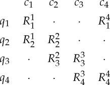
Assuming the numbers of the properties and the contexts are finite, one can present the system of measurements in the form of a matrix, in which rows correspond to the properties {q₁,…,q_n} and columns to the contexts {c₁,…,c_m}, and each cell (i,j) is filled with the measurement if q_i is measured in context c_j (and is left empty otherwise).

3.2

The random variables in any row of this matrix form a connection for the corresponding property, and those in any column form a bunch representing the corresponding context.

We will focus in this paper on a special system of measurements, a cyclic system of rank 4 [1,4,5], or cyclic-4 system for short. Its best-known implementation is the ‘Alice–Bob’ version of the Einstein–Podolsky–Rosen–Bohm system (EPR-B, where B can also stand for Bell). This system has been prominently studied in relation to contextuality since John Bell's pioneering work [18,19], although the conceptual framework used in quantum physics (entanglement, non-locality) initially did not include contextuality explicitly. Outside quantum physics, the term ‘non-locality’ rarely makes sense, and ‘entanglement’, if it does make sense (even if only metaphorical), can always be taken as a possible ‘explanation’ for contextuality, if observed. We will return to the EPR-B implementation of the cyclic-4 system in §8.

The system in question can be presented in the format of the matrix (3.2) as follows:

3.3

We will change the notation later, in §8, to conform with the traditional interpretation of the properties and contexts involved, e.g. in a pair of two entangled particles. For now, one can think of any four properties measured in any four contexts so that (i) each context contains two properties measured together; (ii) each property is measured in two different contexts; (iii) no two contexts share more than one property; and (iv) each measurement is a binary random variable, with values ±1.

4. Traditional understanding of contextuality in cyclic-4 systems

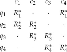
The traditional understanding of contextuality in the cyclic-4 paradigm can be presented as follows. Let us assume the measurements of any property q in the contexts c,c′ in which it is measured to be in fact one and the same random variable, . This assumption can be referred to as that of context-irrelevance, and in many traditional treatments it is made implicitly, by the virtue of indexing the measurements by the properties being measured but not by the contexts. The assumption implies that our matrix (3.3) can be written as

4.1

immediately and trivially implying consistent connectedness: e.g. measured together with in context c₁ is precisely the same random variable as measured together with in context c₄ (otherwise they could not be denoted by the same symbol ); and, of course, a fixed random variable has a fixed distribution.

It is easy to show that if random variables are understood within the framework of the classical, Kolmogorovian probability theory (KPT), then the four random variables in system (4.1) possess a joint distribution. Indeed, the random variables in context c₁ are jointly distributed, which means that they are two measurable functions defined on the same probability space S,

4.2

(More precisely, S is a set in a probability space (S,Σ,μ), where Σ is a sigma-algebra (set of events) on S and μ some probability measure. A function is measurable (and therefore X is a random variable) if the set of values mapped into +1 is an event (i.e. it belongs to Σ, and therefore has a well-defined probability value). We conveniently confuse the set S with the probability space containing S.)

The random variables in context c₄ are also jointly distributed, whence are measurable functions on the same probability space. This must be the same space S as above because the variable in the contexts c₁ and c₄ is the same. Hence

4.3

Finally, in context c₂, the random variables are jointly distributed, and we conclude that

4.4

As a result, all four random variables in (3.3) are measurable functions defined on the same probability space, i.e. they are jointly distributed.

(There is a naive way of arriving at the same conclusion, by assuming that in the KPT any set of random variables is jointly distributed. This view is untenable [9,11].)

Now, the joint distribution of is unobservable, because no two measurements made in two different contexts (such as or ), ‘co-occur’ in any empirical meaning of ‘co-occurrence’. One can only observe (i.e. estimate from observed frequencies of co-occurrences) the distributions of four specific subsets of , the pairs of random variables forming the columns of matrix (4.1). We have the following theorem about these pairs that was first proved, mutatis mutandis, in [20]. In its formulation, 〈⋅〉 denotes expected value, and the maximum is taken over all combinations of + and − signs replacing ± so that the number of the − signs is odd (1 or 3).

Theorem 4.1 —

In any system described by (4.1),

4.5

The above inequality is usually presented as a necessary condition for the existence of a joint distribution of , implying that (4.5) can be violated, in which case do not have a joint distribution and we say that the cyclic-4 system is contextual. This understanding, however, lacks logical rigour. If the left-hand side of (4.5) can be computed at all, then the expected products in it are well defined, whence each of the corresponding pairs has a well-defined joint distribution. But then, as we have seen, the entire set has to have a joint distribution too, and then, by theorem 4.1, (4.5) must hold. It simply cannot be violated.

Put differently but equivalently, if do not possess a joint distribution, then at least two of the four pairs forming columns of matrix (4.1) do not have joint distributions (because a global joint distribution follows from any three of these pairs being jointly distributed). But if this is the case, the left-hand side of (4.5) simply cannot be computed.

5. Consistent connectedness and contextuality in traditional understanding

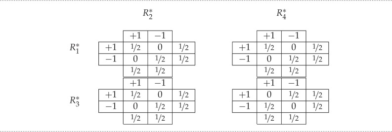
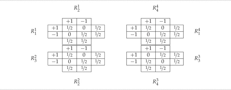
One can be easily confused by the reasoning above, because it may seem that it is trivial to construct a system (4.1) in which all four expected products are well defined while (4.5) is violated (and it is routinely claimed that quantum mechanics predicts such situations and experiments confirm these predictions). This seemingly trivial possibility, however, is merely an illusion, because such a construction would be one of a mathematically self-contradictory system. One example is given by the four distributions in table 1, where entries within the 2×2 interiors are joint probabilities, while the margins show marginal probabilities. The expected products here are

and the left-hand side of (4.5) is 4, violating the inequality. As this system is mathematically impossible, we must have made an assumption that this contradiction demonstrates to be false.

Table 1.

Example in which the left-hand side of (4.5) is seemingly well defined and exceeds 2. Since this is mathematically impossible, there should be a hidden assumption here that is false.

What might this assumption be? Can it be that are are not jointly distributed, or that they are not well-defined random variables? The answer is clearly negative: are are observed empirically and jointly. The same reasoning applies to the remaining three pairs: in each pair, the two random variables are well defined and jointly distributed. The only possible error therefore is in the identity of these random variables across different contexts: we have assumed, e.g., that measured together with is the same random variable as measured together with . It must be wrong to label the measurements by the measured properties only, ignoring the contexts.

This means that a correct initial representation of the system would be as in table 2, with the random variables contextually labelled, so that the pairs of measurements forming different bunches do not overlap. If one makes the assumption that, for any property q and any two contexts c,c′, the measurements and in this matrix are ‘one and the same variable’ , then this assumption is rejected by reductio ad absurdum: if it were correct, (4.5) would have to hold, and it does not.

Table 2.

Example of table 1 without the assumption of context-irrelevance: the identity of measurements (random variables) depends not only on what is measured but also on the context in which it is measured.

Below we will present a rigorous way of formulating the hypothesis that random variables measuring the same property in different contexts are (in some sense) ‘the same’. We already have, however, sufficient clarity about this hypothesis to address the often misunderstood question of the relationship, within the framework of this hypothesis, between the concepts of consistent connectedness and contextuality.

It is clear that the assumption of consistent connectedness can be formulated and, in special cases, even justified without assuming context-irrelevance. Its formulation for the cyclic-4 system presented in the form (3.3) is

5.1

Such a hypothesis can often be entertained without assuming that the identically distributed random variables are ‘the same’. For instance, in the classical entanglement paradigm for two electrons, property 1 corresponds to Alice's choice of a certain axis in her particle, and the context c₁ is defined by Bob's simultaneously choosing axis 2 in his particle, while the context c₄ is defined by Bob's simultaneously choosing axis 4 (on labelling Alice's two axes 1,3 and Bob's two axes 2,4). If the two particles are space-like separated, one should assume that Bob's settings cannot influence Alice's measurements, which implies the distribution of is the same as the distribution of . No physical principle prevents one, however, from viewing and as different random variables with one and the same distribution. We have seen already that one's denying this view leads to a mathematical contradiction.

The expected products in (4.5) also can be written without regard to the context-irrelevance hypothesis. One can replace with , with , etc., to obtain the following analogue of inequality (4.5):

5.2

Using this formulation, theorem 4.1 can be understood as stating that (5.2) holds under the context-irrelevance hypothesis. If this hypothesis does not hold, (5.2) does not have to be satisfied and therefore cannot be derived as a theorem. One can always check whether it holds or not, but the outcome has no known to us interpretation if and are not assumed always to be the same. Now, the context-irrelevance hypothesis simply cannot be entertained if consistent connectedness is violated: ‘one and the same’ random variable cannot have two different distributions. There is therefore no reason for checking the inequality (5.2) if (5.1) does not hold.

The only exception can be made in an imaginary situation wherein the consistency of connectedness is not known (e.g. it is not established in a statistically reliable way), but one knows (in a statistically reliable way) that the inequality (5.2) is violated. In this case, one can reject the context-irrelevance hypothesis by the following reasoning: (i) if the system is consistently connected, then the hypothesis of context-irrelevance leads to (5.2), which is rejected; (ii) if the system is not consistently connected, the hypothesis of context-irrelevance is rejected as well; (iii) hence this hypothesis is rejected.

6. Traditional understanding of contextuality translated into the contextuality-by-default language

In accordance with the CbD approach, and (c≠c′) are a priori different random variables, and since they are never observed ‘together’ (in any empirically grounded sense of this word), they do not posses a joint distribution. The conceptual coherence and advantages offered by this understanding of random variables recorded in different contexts has been discussed in [1,9,21]. In the framework of KPT this means that and are functions defined on two different probability spaces:

6.1

It is therefore impossible to hypothesize that and (c≠c′) are in fact ‘the same’. Nor is it possible to treat these and as ‘different but always equal to each other’,

6.2

since this statement also implies a joint distribution of , translating into S_c=S_c′.

To formulate the analogue of the context-irrelevance hypothesis within the framework of CbD, one has to use the foundational notion of a (probabilistic) coupling.

Definition 6.1 —

A coupling for the cyclic-4 system (3.3) is a set of eight jointly distributed random variables

6.3

such that

6.4

In other words, the bunches of the system are distributed as the corresponding marginals of the coupling. A system has generally an infinity of couplings.

The notion of a coupling is not confined to cyclic-4 systems. It applies to any system of random variables, the idea being that (i) the coupling is a set of jointly distributed random variables in a one-to-one correspondence with the variables constituting the system being coupled and (ii) the observable parts of this system are distributed in the same way as the corresponding marginals (subsets, or subcouplings) of the coupling. In particular, the system being coupled can be a connection of the cyclic-4 system.

Recall that the connection for property q is the set of all random variables measuring q in different contexts. In the cyclic-4 system, the connection for property 1 is , for property 2 it is , etc., along the rows of the matrix (3.3). Each of these connections taken in isolation has its couplings.

Definition 6.2 —

A pair of jointly distributed random variables is a coupling of a connection in a cyclic-4 system if

6.5

The coupling is called maximal if the probability with which attain equal values, , is maximal among all couplings of .

Another way of stating the second part of the definition is that is as large as it is allowed to be by the distributions of and , which are fixed by (6.5). The following theorem says that this concept is well defined.

Theorem 6.3 (Refs. [1,4]). —

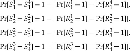
A maximal coupling of a connection in a cyclic-4 system exists and its distribution is unique: it is defined by (6.5) and

6.6

or equivalently,

6.7

The notion of a maximal coupling and the existence part of the theorem above can be generalized to arbitrary systems [2,4,21], but in this paper we focus on the cyclic-4 systems only.

It is easy to see that if a cyclic-4 system is consistently connected, i.e. if for all q,c,c′, then in a maximal coupling of any connection we have , or equivalently,

6.8

In other words, in a maximal coupling the measurements in a connection are modelled as being essentially ‘the same’. This simple observation allows us to make use of the notion of maximal couplings in the following rigorous version of the traditional understanding of contextuality.

Definition 6.4 —

A consistently connected cyclic-4 system (3.3) is non-contextual if it has a coupling (6.3) in which are maximal couplings for the corresponding connections , i.e. if

6.9

If such a coupling does not exist, the system is contextual.

This definition allows one to preserve the spirit of the traditional understanding (the context-irrelevance hypothesis: and are always ‘the same’) while adhering to the logic of the CbD approach: and are not only different, they are not even stochastically interrelated. From this point of view, the following theorem, first proved mutatis mutandis by Fine [22,23], summarizes the traditional analysis of contextuality for the cyclic-4 systems.

Theorem 6.5 —

A consistently connected cyclic-4 system (3.3) is non-contextual (by definition 6.4) if and only if (5.2) is satisfied.

This is a special case of theorem 7.2 below, which in turn is a special case of a theorem proved in [5] (see also [1,2,4,21]) that applies to a broad class of cyclic systems, of which cyclic-4 ones are a special case.

7. A general definition and criterion of contextuality in the contextuality-by-default framework

The fact that we relate definition 6.4 to the notion of maximal couplings for connections reflects the intuition we are guided by and suggests a natural way of generalizing contextuality beyond consistently connected systems.

The intuition in question can be explicated as follows. For an inconsistently connected system, we interpret the non-coincidence of the distributions of and as evidence that changes in context, , ‘directly’ influence the measurement of q. For instance, in the Alice–Bob entanglement paradigm, if the two measurements are time-like separated, Alice's choice of the spin axis can influence Bob's measurement along a given axis. This is referred to as ‘signalling’. It is also possible that a Charlie who receives information from both Alice and Bob and records both their settings and their measurement results makes systematic errors in recording Bob's results depending on Alice's settings. This is referred to as ‘context-dependent biases’. Whatever the cause, when we model these ‘direct’ influences by a coupling of , we translate the differences in distributions into differences in values: as c changes into c′, the value of changes into a corresponding value of . In a maximal coupling, we do this in the maximally conservative way: the values of and remain the same as often as it is allowed by their individual distributions (in particular, they remain always the same if the distributions are the same). Modelling by such a coupling is always possible if is coupled in isolation. Now, if this is also possible for all the connections taken together, within the framework of an overall coupling of the entire system, we can say that direct influences are sufficient to account for the system. If, however, this is not possible, then the maximal couplings for different connections are not mutually compatible: we interpret this as evidence that we need more than direct influences to account for the system. This ‘more’ is what we call contextuality, as distinct from direct influences.

The generalization of definition 6.4 to arbitrary systems of measurement therefore is straightforward: one can simply drop the qualification ‘consistently connected’ and use the general form of theorem 6.3.

Definition 7.1 —

A cyclic-4 system (3.3) is non-contextual if it has a coupling (6.3) in which are maximal couplings for the corresponding connections , i.e. if

7.1

This is arguably the most conservative generalization of definition 6.4, but it is sufficient to deal with all conceivable cyclic-4 systems. The correspondingly generalized version of theorem 6.5 is as follows [1,4,5,12].

Theorem 7.2 —

A cyclic-4 system (3.3) is non-contextual if and only if

7.2

where

7.3

and

7.4

The abbreviations in this theorem are as follows. CHSH is the left-hand side expression in the classical Clauser–Horn–Shimony–Holt (CHSH) inequality (5.2), named so after the authors of [20]. ICC is a measure of inconsistency of the connectedness [1,4,12]: if it is zero, then the criterion (7.2) reduces to the CHSH inequality (5.2), and the theorem above reduces to theorem 6.5.

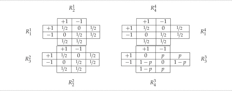
To illustrate the computations, consider the modification of the example of table 2 in table 3. The value of CHSH in the system is 4, the same maximal possible value as in table 2. But

whence

The system is non-contextual by the criterion (7.2) only if p=0 or p=1; for other values the difference exceeds 2.

Table 3.

An inconsistently connected cyclic-4 system. In accordance with the general definition 7.1, the system is contextual if and only if p is not 0 or 1. In accordance with the narrow (traditional) definition 6.4, the notion of contextuality is not applicable unless p=1/2; in all other cases the criterion (5.2) is not derivable and the value of CHSH is not interpretable.

One can see in (7.2) an algebraic realization of the intuition described above, of direct influences being or not being sufficient to account for the system. The direct influences are represented by the term ICC while CHSH−2 can be viewed as the total of the dependence of measurements on contexts. If ICC is not large enough, it does not exceed CHSH−2, and in this sense it is ‘insufficient’ to explain the total of the context-dependence. The difference is the ‘unexplained’ context-dependence that we view as true contextuality.

For the arguments in favour of generalizing the definition of contextuality to inconsistently connected systems, see [1,4,21]. Let us emphasize here a pragmatic argument. Since one cannot prove a null hypothesis, dealing with experimental results one can never be certain that consistent connectedness holds. If one confines one's definition of contextuality to the latter case (definition 6.4), one's determination that a system is contextual would always be ‘suspended’ and could be easily invalidated if with a larger sample size a small inconsistency were detected. Moreover, small inconsistencies should be expected in virtually all real experiments, as one can never be rid of all systematic sources of error or make them perfectly counterbalanced. None of this poses a problem for definition 7.1: small values of ICC, unless CHSH is very close to 2, will not change one's determination that a system is or is not contextual.

8. The ‘Alice–Bob’ EPR-B version of the cyclic-4 system

The contextuality analysis of a cyclic-4 system does not depend on what precisely the properties {q₁,q₂,q₃,q₄} are, nor on what the contexts {c₁,c₂,c₃,c₄} are. All that matters is that each context involves two properties measured ‘together’, no two contexts share more than one property, each property is measured in precisely two different contexts, and each measurement has two possible values.

The importance of the cyclic-4 systems, however, is primarily related to the entanglement paradigm in quantum mechanics: two particles created in a singular state move away from each other, reaching simultaneously two observers, one of them Alice and another Bob; Alice chooses one of two fixed axes and measures her particle's spin along it; Bob does the same with his particle. Assuming the two particles are spin- ones, the outcomes are binary random variables. Alice's two fixed axes can be denoted a₁=q₁ and a₂=q₃, and Bob's axes can be denoted b₁=q₂ and b₂=q₄. The contexts then can be identified by the pairs of axes simultaneously chosen by Alice and Bob:

8.1

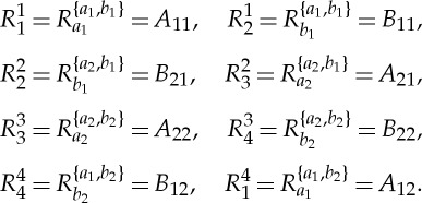
We can now simplify notation for the measurements by denoting Alice's measurements by A and Bob's by B. We will use two subscripts of which (note the asymmetry) the first one refers to Alice's choice of one of her two axes, and the second one refers to Bob's choice of one of his two axes. This notation ensures that A_ij and B_ij (and only these, identically subscripted pairs) are jointly distributed. Random variable A_ij is interpreted as the outcome of measuring property a_i in the context of being measured together with property b_j (whether or not the distribution of A_ij depends on j); B_ij is the outcome of measuring property b_j in the context of being measured together with property a_i (whether or not the distribution of B_ij depends on i).

The correspondence between the general notation and the special A_ij–B_ij notation is as follows:

8.2

The entanglement paradigm serves as a template for other applications, with very different meanings of the properties a,b (see [3] for examples in psychology). In this paper, we will use as an example the experiment by Aerts & Sozzo [6], where a and b are cardinal and intercardinal orientations, respectively, chosen in the Rose of the Winds, and the measurements are choices (by human respondents) of one of two possible wind directions along each of these orientations, as shown in table 4.

Table 4.

The properties and their measurements in the EPR-B-like system used in [6]. In each trial, a human respondent is asked to choose ‘wind directions’ along a pair of spatial orientations in the Rose of the Winds. Each pair consists of one cardinal orientation (a₁ or a₂) and one intercardinal orientation (b₁ or b₂). For instance, the respondent can be given (a₂,b₁), in which case her possible choices would be ‘East and Northeast’, ‘East and Southwest’, ‘West and Northeast’ and ‘West and Southwest’, corresponding to four possible values of (A₂₁,B₂₁).

properties, q (Rose of the Winds)	measurements (choices of direction)	context (options for other direction)
North–South (a1)	A1j=+1=North	measured together with bj ( j=1,2)
	A1j=−1=South
East–West (a2)	A2j=+1=East
	A2j=−1=West
Northeast–Southwest (b1)	Bi1=+1=Northeast	measured together with ai (i=1,2)
	Bi1=−1=Southwest
Northwest–Southeast (b2)	Bi2=+1=Southeast
	Bi2=−1=Northwest

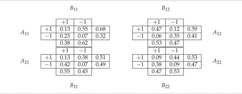
The results of this experiment (table 5) yield the following computations:

whence

We conclude that the data exhibit no contextuality in the sense of definition 7.1.

Table 5.

The results of the experiment reported in [6]. All probability estimates are computed from polling 85 people, treating them as 85 realizations of one and the same pair of random variables in each of the four contexts.

9. Methodological remarks

One may, of course, reject the generalized definition 7.1 and stick with the traditional understanding (definition 6.4), but the latter applies only to consistently connected systems of measurements, whereas the inconsistency of the connectedness in the data of [6] is clearly present in spite of the small sample size used (p<0.03 for the difference between 〈B₁₁〉 and 〈B₂₁〉). As explained in §5, in this case no inequality can be derived for CHSH (except for the trivial CHSH≤4), and no interpretation is known for whether CHSH exceeds or does not exceed any value below 4.

The authors of [6] are aware of the difficulties caused by inconsistent connectedness in judging violations of the CHSH inequality [7], so they propose a computational modification of their data that makes all marginal distributions uniform. They justify this procedure by an isotropy argument, according to which any direction in the Rose of the Winds plane could be taken to play the role of the vector North, with all other directions rotated to preserve their angles with respect to this new North. Using this argument, Aerts and Sozzo average the observed probabilities in such a way that all marginal probabilities become while the value of CHSH does not change.

An isotropy argument, however, as any other symmetry argument, only makes sense if formulated as invariance of a relevant feature (in our case, measurement) with respect to certain changes. To give a trivial example, the length of a segment in the Euclidean plane is invariant with respect to its rotations. Therefore, one can average the length measurements of a radius at different orientations, and this averaging would only improve statistical reliability of the measurements rather than change the true measured value. By contrast, we see in table 5 that the measurements A_ij and B_ij are not invariant with respect to rotations: e.g. is different from , although the ordered pair of the orientations in the second case, (b₁,a₂), is a rotated by π/4 copy of the orientation pair in the first case, (a₁,b₁). Even more obvious: is not the same as although they pertain to orientation pairs rotated by π with respect to each other.

The latter example is important for the computational modification of the data used in [6]. This procedure achieves uniform marginals while retaining the value of CHSH precisely because it considers the jointly-opposite outcomes

9.1

with x,y∈{−1,+1}, to be ‘equivalent’. The probability of each of them is therefore replaced with their average:

9.2

Let us denote by and the new random variables with these symmetrized distributions. Owing to the symmetry,

9.3

At the same time,

9.4

and since it follows from (9.2) that

9.5

the value of CHSH remains intact.

This averaging procedure has been described in the quantum physics literature by Masanes et al. [24]; it is the first part of their ‘depolarization’ procedure. There, however, it is meant to be a data generation or data doctoring procedure (not a data analysis one), involving either direct signalling between Alice or Bob, or a third party, Charley, who receives from Alice and from Bob their settings and their measurement results, flips a fair coin, and multiplies these measurement results (always both of them) by +1 or −1 accordingly. Since this averaging procedure is universal (applicable to all EPR-B systems without exception), if taken as a data analysis procedure it amounts to ignoring the marginal probabilities altogether and simply defining contextuality (or entanglement) as any violation of the CHSH inequality.

One might ask: why not adopt this approach? It is definitely simpler than the approach advocated by us, which involves (i) labelling the measurements contextually, (ii) determining subsystems of measurements that are stochastically unrelated to each other, (iii) defining contextuality in terms of the (non)existence of a coupling for these subsystems with certain constraints imposed on the connections (measurements of the same properties in different contexts), and (iv) deriving CHSH inequalities or their generalizations as theorems [1,2,4,5,9–11,21].

The answer to the question is that adopting the definition in question, in addition to being arbitrary, would make construction of contextual systems child's play: the contextual system will become ubiquitous and obvious, including systems in classical mechanics and human behaviour that no one normally would think of as contextual. Moreover, with the definition in question one would have to forget about the ‘quantum’ motivation for seeking contextuality, because these contextual systems in classical mechanics and human behaviour would violate Tsirelson (or Cirel'son) bounds [25,26] as easily as they would the CHSH ones.

10. Contextuality as child's play

We will consider just one example, with multiple possible implementations. Table 6 represents the probabilities of [A_ij=x,B_ij=y] in a hypothetical EPR-B-type system (i,j∈{1,2}, x,y∈{−1,+1}). Here,

the algebraically maximal possible value for CHSH. The system is, however, non-contextual by definition 7.1 and theorem 7.2: ICC in it equals the value of 〈A₂₁〉−〈A₂₂〉=2, whence

In fact, any deterministic system (one in which all probabilities are 0 or 1) is non-contextual. A simple way of demonstrating this is as follows: a deterministic system has a single coupling, and its subcouplings corresponding to connections (each of which is deterministic) are their only couplings, hence maximal ones.

Table 6.

A deterministic system that is (as any other deterministic system) non-contextual by definition 7.1 but is ‘maximally contextual’ if one ignores marginal probabilities (or, equivalently, averages over jointly opposite outcomes).

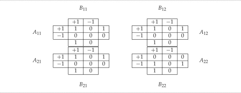However, if in table 6 one decides to ignore marginal probabilities, the system is maximally contextual (and in fact more contextual than allowed by quantum mechanics).

It is trivial to find or construct a system described by table 6. To begin with conceptual combinations, consider e.g. the experiment in which the properties a,b and measurements A,B are identified as shown in table 7. Such an experiment would yield table 6 unless the participants choose to deliberately give wrong responses. There is, in fact, nothing wrong in considering the conceptual inferences like ‘Green Triangle is Green’ and ‘Green Triangle is Triangular’ as examples of contextuality or ‘(super-quantum) entanglement,’ but this looks to us as making the concept of contextuality too trivial to be of interest.

Table 7.

A trivial system described by table 6 if people are instructed to choose correct responses. In the context (a₁,b₁), the choice is among the sentences: ‘Green Triangle is Green’, ‘Green Triangle is Red’, ‘Yellow Circle is Green’ and ‘Yellow Circle is Red’. In the context (a₁,b₂) the choice is among the sentences: ‘Green Triangle is Triangular’, ‘Green Triangle is Square’, ‘Yellow Circle is Triangular’ and ‘Yellow Circle is Square’. In the context (a₂,b₁), the choice is among the sentences: ‘Green Circle is Green’, ‘Green Circle is Red’, ‘Yellow Triangle is Green’ and ‘Yellow Triangle is Red’. In the context (a₂,b₂), the choice is among the sentences: ‘Green Circle is Triangular’, ‘Green Circle is Square’, ‘Yellow Triangle is Triangular’ and ‘Yellow Triangle is Square’.

properties (choices between)	measurements (choices)	context
Green Triangle and Yellow Circle (a1)	A1j=+1=Green Triangle	together with bj ( j=1,2)
	A1j=−1=Yellow Circle
Green Circle and Yellow Triangle (a2)	A2j=+1=Green Circle
	A2j=−1=Yellow Triangle
Green and Red (b1)	Bi1=+1=Green	together with ai ( j=1,2)
	Bi1=−1=Red
Triangular and Square (b2)	Bi2=+1=Triangular
	Bi2=−1=Square

Another example of ‘conceptual entanglement’ involves creation of new concepts in children by means of teaching them a simple nonsense verse:

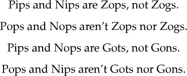Children who learned this piece of poetry by heart (or are allowed to look at it while responding) would confidently respond to the questions like ‘Are Pips Zops?’ and ‘Are Pops Gots?’ The resulting table of the probabilities for them will be the same as in table 6, on denoting the conditions and outcomes as in table 8.

Table 8.

A trivial system described by table 6 if people are instructed to choose correct responses given by the nonsense verse about Pips, Nips, etc.

properties (choices between)	measurements (choices)	context
Pip and Pop (a1)	A1j=+1=Pip	together with bj ( j=1,2)
	A1j=−1=Pop
Nip and Nop (a2)	A2j=+1=Nip
	A2j=−1=Nop
Zop and Zog (b1)	Bi1=+1=Zop	together with ai (i=1,2)
	Bi1=−1=Zog
Got and Gon (b2)	Bi2=+1=Got
	Bi2=−1=Gon

Finally, here is a scenario of creating table 6 in a purely classical physical situation. There is a gadget ‘Alice’ that responds to inputs i,j∈{1,2} by computing , and a gadget ‘Bob’ that outputs 1 no matter what. This example is essentially identical to one given by Filk in fig. 3 of [27]. No physicist, as it seems to us, would call the system consisting of these two gadgets entangled or contextual. It is simply that both inputs influence one of the outputs (Alice's), resulting in the observed inconsistent connectedness.

11. Conclusion

Inconsistent connectedness is almost a universal rule in behavioural and social data (e.g. it is very plausible that the task of choosing between the North and South winds affects the probabilities with which one, in the same trial, chooses between the Northeast and Southwest winds). It is therefore a sound scientific strategy to make inconsistent connectedness part of one's theory of contextuality. Inconsistent connectedness means that the measurement of a property is directly influenced by the measurement of other properties, and this may or may not be sufficient to account for a system's behaviour. For instance, in the experiment described in [28], we find violations of consistent connectedness due to context-dependent biases in measurements, but the detailed analysis presented in [4] shows that contextuality, in the sense of definition 7.1, is still prominently present in these data. By contrast, the system in table 6 is non-contextual by definition 7.1, which means that the direct influences it entails are sufficient to explain its behaviour (no contextuality exists ‘on top of’ these input–output relations). The same conclusion applies to the many different experiments analysed in [3] and to the experiment reported in [6]. We have argued that the justification proposed in the latter for averaging across different contexts is not tenable, and the reason it works as desired is that it is equivalent to ignoring marginal probabilities altogether. The consequence of such ignoring, in addition to being ad hoc, is that contextuality becomes trivial and uninteresting.

We make no claim, however, that contextuality, in the sense of our definition, cannot be found in behavioural data: we merely say that we have not found it yet. We also acknowledge that there may be viable alternatives to our definition 7.1 that also take into account inconsistent connectedness in a different way.

Finally, we would like to refer the reader to the concluding part of [3] to emphasize that absence of contextuality in behavioural and social systems does not mean that quantum formalisms are not applicable to them. The so-called QQ equality, in our opinion the most impressive outcome of quantum cognition research to date [29,30], provides a clear illustration of how absence of contextuality can in fact be precisely a prediction derived from quantum theory.

Authors' contributions

All authors significantly contributed to writing of the paper. The mathematical theory was developed primarily by J.V.K. and E.N.D.

Competing interests

We declare we have no competing interests.

Funding

This research has been supported by NSF grant no. SES-1155956, AFOSR grant no. FA9550-14-1-0318, A. von Humboldt Foundation and the J. William Fulbright Grant from Fulbright Colombia.

References

- 1.Dzhafarov EN, Kujala JV, Larsson J- Å. 2015. Contextuality in three types of quantum-mechanical systems. Found. Phys. 7, 762–782. ( 10.1007/s10701-015-9882-9) [DOI] [Google Scholar]
- 2.Dzhafarov EN, Kujala JV, Cervantes VH. 2016. Contextuality-by-default: a brief overview of ideas, concepts, and terminology. Lect. Notes Comput. Sci. 9535, 12–23. ( 10.1007/978-3-319-28675-4_2) [DOI] [Google Scholar]
- 3.Dzhafarov EN, Zhang R, Kujala JV. 2016. Is there contextuality in behavioral and social systems? Phil. Trans. R. Soc. A 374, 20150099 ( 10.1098/rsta.2015.0099) [DOI] [PubMed] [Google Scholar]
- 4.Kujala JV, Dzhafarov EN, Larsson J- Å. 2015. Necessary and sufficient conditions for maximal noncontextuality in a broad class of quantum mechanical systems. Phys. Rev. Lett. 115, 150401 ( 10.1103/PhysRevLett.115.150401) [DOI] [PubMed] [Google Scholar]
- 5.Kujala JV, Dzhafarov EN.2015. Proof of a conjecture on contextuality in cyclic systems with binary variables. (http://arxiv.org/abs/1503.02181. )
- 6.Aerts D, Sozzo S.2015. Spin and wind directions: identifying entanglement in nature and cognition. (http://arxiv.org/abs/1508.00434v2. )
- 7.Dzhafarov EN, Kujala JV. 2014. Selective influences, marginal selectivity, and Bell/CHSH inequalities. Top. Cogn. Sci. 6, 121–128. ( 10.1111/tops.12060) [DOI] [PubMed] [Google Scholar]
- 8.Aerts D, Gabora L, Sozzo S. 2013. Concepts and their dynamics: A quantum-theoretic modeling of human thought. Top. Cogn. Sci. 5, 737–772. ( 10.1111/tops.12042) [DOI] [PubMed] [Google Scholar]
- 9.Dzhafarov EN, Kujala JV. 2014. Contextuality is about identity of random variables. Phys. Scripta T163, 014009 ( 10.1088/0031-8949/2014/T163/014009) [DOI] [Google Scholar]
- 10.Dzhafarov EN, Kujala JV. 2014. Embedding quantum into classical: contextualization vs conditionalization. PLoS ONE 9, e92818 ( 10.1371/journal.pone.0092818) [DOI] [PMC free article] [PubMed] [Google Scholar]
- 11.Dzhafarov EN, Kujala JV. 2014. A qualified Kolmogorovian account of probabilistic contextuality. Lect. Notes Comput. Sc. 8369, 201–212. ( 10.1007/978-3-642-54943-4_18) [DOI] [Google Scholar]
- 12.Kujala JV, Dzhafarov EN. 2015. Probabilistic Contextuality in EPR/Bohm-type systems with signaling allowed. In Contextuality from quantum physics to psychology (eds EN Dzhafarov, JS Jordan, R Zhang, VH Cervantes), pp. 287–308. Hackensack, NJ: World Scientific Press.
- 13.Popescu S, Rohrlich D. 1994. Quantum nonlocality as an axiom. Found. Phys. 24, 379–385. ( 10.1007/BF02058098) [DOI] [Google Scholar]
- 14.Dzhafarov EN, Kujala JV. 2012. Quantum entanglement and the issue of selective influences in psychology: an overview. Lect. Notes Comput. Sc. 7620, 184–195. ( 10.1007/978-3-642-35659-9_17) [DOI] [Google Scholar]
- 15.Townsend JT, Schweickert R. 1989. Toward the trichotomy method of reaction times: laying the foundation of stochastic mental networks. J. Math. Psychol. 33, 309–327. ( 10.1016/0022-2496(89)90013-8) [DOI] [Google Scholar]
- 16.Ramanathan R, Soeda A, Kurzynski P, Kasznlikowski D. 2012. Generalized monogamy of contextual inequalities from the no-disturbance principle. Phys. Rev. Lett. 109, 050404 ( 10.1103/PhysRevLett.109.050404) [DOI] [PubMed] [Google Scholar]
- 17.Cereceda J. 2000. Quantum mechanical probabilities and general probabilistic constraints for Einstein–Podolsky–Rosen–Bohm experiments. Found. Phys. Lett. 13, 427–442. ( 10.1023/A:1007828731477) [DOI] [Google Scholar]
- 18.Bell JS. 1964. On the Einstein–Podolsky–Rosen paradox. Physics 1, 195–200. [Google Scholar]
- 19.Bell JS. 1966. On the problem of hidden variables in quantum mechanics. Rev. Mod. Phys. 38, 447–453. ( 10.1103/RevModPhys.38.447) [DOI] [Google Scholar]
- 20.Clauser JF, Horne MA, Shimony A, Holt RA. 1969. Proposed experiment to test local hidden-variable theories. Phys. Rev. Lett. 23, 880–884. ( 10.1103/PhysRevLett.23.880) [DOI] [Google Scholar]
- 21.Dzhafarov EN, Kujala JV. 2015. Conversations on contextuality. In Contextuality from quantum physics to psychology (eds EN Dzhafarov, JS Jordan, R Zhang, VH Cervantes), pp. 1–22, Hackensack, NJ: World Scientific Press.
- 22.Fine A. 1982. Joint distributions, quantum correlations, and commuting observables. J. Math. Phys. 23, 1306–1310. ( 10.1063/1.525514) [DOI] [Google Scholar]
- 23.Fine A. 1982. Hidden variables, joint probability, and the Bell inequalities. Phys. Rev. Lett. 48, 291–295. ( 10.1103/PhysRevLett.48.291) [DOI] [Google Scholar]
- 24.Masanes Ll, Acin A, Gisin N. 2006. General properties of nonsignaling theories. Phys. Rev. A 73, 012112 ( 10.1103/PhysRevA.73.012112) [DOI] [Google Scholar]
- 25.Cirel'son BS. 1980. Quantum generalizations of Bell's inequality. Lett. Math. Phys. 4, 93–100. ( 10.1007/BF00417500) [DOI] [Google Scholar]
- 26.Landau LJ. 1987. On the violation of Bell's inequality in quantum theory. Phys. Lett. A 120, 54–56. ( 10.1016/0375-9601(87)90075-2) [DOI] [Google Scholar]
- 27.Filk T. 2015. It is the theory which decides what we can observe. In Contextuality from quantum physics to psychology (eds EN Dzhafarov, JS Jordan, R Zhang, VH Cervantes), pp. 77–92, Hackensack, NJ: World Scientific Press.
- 28.Lapkiewicz R, Li P, Schaeff C, Langford NK, Ramelow S, Wieśniak M, Zeilinger A. 2011. Experimental non-classicality of an indivisible quantum system. Nature 474, 490–493. ( 10.1038/nature10119) [DOI] [PubMed] [Google Scholar]
- 29.Wang Z, Solloway T, Shiffrin RM, Busemeyer JR. 2014. Context effects produced by question orders reveal quantum nature of human judgments. Proc. Natl Acad. Sci. USA 111, 9431–9436. ( 10.1073/pnas.1407756111) [DOI] [PMC free article] [PubMed] [Google Scholar]
- 30.Wang Z, Busemeyer JR. 2013. A quantum question order model supported by empirical tests of an a priori and precise prediction. Top. Cogn. Sci. 5, 689–710. ( 10.1111/tops.12040) [DOI] [PubMed] [Google Scholar]