Three-body system metaphor for the two-slit experiment and Escherichia coli lactose–glucose metabolism

Abstract

We compare the contextual probabilistic structures of the seminal two-slit experiment (quantum interference experiment), the system of three interacting bodies and Escherichia coli lactose–glucose metabolism. We show that they have the same non-Kolmogorov probabilistic structure resulting from multi-contextuality. There are plenty of statistical data with non-Kolmogorov features; in particular, the probabilistic behaviour of neither quantum nor biological systems can be described classically. Biological systems (even cells and proteins) are macroscopic systems and one may try to present a more detailed model of interactions in such systems that lead to quantum-like probabilistic behaviour. The system of interactions between three bodies is one of the simplest metaphoric examples for such interactions. By proceeding further in this way (by playing with n-body systems) we shall be able to find metaphoric mechanical models for complex bio-interactions, e.g. signalling between cells, leading to non-Kolmogorov probabilistic data.

1. Introduction

The two-slit experiment demonstrating the interference of probabilities lies at the heart of quantum foundations. We note that, for example, Feynman pointed to this experiment in practically all foundational discussions. In particular, he emphasized its non-classical probabilistic structure [1]. (It seems that Feynman was not aware of the modern measure-theoretic formulation of classical probability theory [2] and he referred to Laplace probability theory.) He highlighted the contextual structure of this experiment as the source of non-classicality and demonstrated by using the calculus of complex probability amplitudes (wave functions) that the basic law of classical probability theory, additivity of probability, is violated for data collected for three experimental contexts, C_i, i=1,2, only the ith slit is open, and C₁₂, both slits are open. This violation of additivity can be reformulated in terms of conditional probabilities [3] (which is more useful in the framework of probability inference) as violation of the formula of total probability (FTP).

Thus, the mathematical quantum formalism can be treated as one possible way to work with non-Kolmogorov probability (NKP). From this point of view, we can stress that the formalism of quantum mechanics is not just a physical theory but also a probability theory. We can apply NKP to non-physical phenomena which violate the additivity in classical probability theory. We can find many applications of quantum probability outside of physics, e.g. the application of quantum interference to psychological experiments [4,5] and the application of quantum mechanical dynamics to the Black–Scholes option pricing model in finance theory [6,7].

Recently, it was shown that many biological phenomena, such as metabolism, differentiation, evolution, adaptation and cognition, violate the FTP [3,8,9] (as well as another consequence of the classical Kolmogorov probability model—the Bell inequality [10], which plays a key role in modern debates on quantum foundations [11]; see [12] on the violation of the Bell-type inequalities in the process of recognition of ambiguous figures). As in the case of quantum physics, in biology the contextuality of behaviour is the source of the NKP structure of statistical experimental data. Bio-contextuality results from the adaptivity of bio-systems to the environment (in particular, to experimental contexts). By comparing the NKP features of the behaviour of bio-systems and quantum physical systems, one may try to apply mathematical quantum formalism to model probabilistic biological behaviour. We emphasize that the use of this formalism is just a possibility, not a necessity. Other NKP models may be used as well, e.g. non-additive probabilities [13]. In this study, we shall not discuss the advantages and disadvantages of the use of quantum probability (see [14,15] for a review). In [3,9,16–18], there are discussions on the availability of quantum mechanical formalism. Here, in this paper, we discuss only the following foundational problem. Bio-systems are macroscopic systems compared with the scales of quantum mechanics—even proteins and cells are huge compared with electrons and atoms. Therefore, in principle, their behaviour can be described by using classical physical and chemical interactions; for example, molecular biology studies of signalling in molecular networks inside a cell and neurophysiology in networks of firing neurons. Thus, although the probabilistic structures of quantum physical and quantum-like biological models are similar, functionally they are different, because in quantum mechanics we cannot generate probabilistic behaviour by using models with classical physical and chemical interactions—there are ‘no hidden variables’ (at least this is the common viewpoint; see, however, for example [19] for debates).

The aim of this article is to demonstrate that classical mechanical interactions inside sufficiently simple physical systems can generate NKP behaviour. It is easier to model mechanical interactions and derive from them the NKP output than to model interactions in even the simplest bio-systems, such as cells. Macroscopic biological processes involved in biological phenomena are usually deterministic, but they operate under a many complex interaction (information transduction) network [18,20]. The mathematical formulations of such macroscopic complex systems, including the complex network system of metabolism in a bacterium, require tremendous efforts (e.g. [21]).

Our aim is to determine that NKP behaviour can arise from a classical system accompanied by complicated interactions. In this sense, the three-body system can be a candidate for a metaphoric mechanical model of such NKP behaviour. The two-body problem, such as the typical Sun/Earth relation under gravity, can be mathematically described by the deterministic Newton's equation of motion. However, the three-body system is known not to be able to be solved analytically, although it is deterministic. This is because it contains more than two interactions. (It is surprising that the transition from two to three interactions results in a tremendous increase in the complexity of behaviour.)

In this study, we demonstrate the NKP features of the simplest physical system of three linearly connected balls, which is a special case of the three-body system. We try to apply our NKP theory to understand the fundamental property of the phenomenon observed in the three-body problem, but do not aim to solve the three-body behaviour itself. And this simple example will aid in understanding the fundamentals of our NKP applied to a complex system with many interacting components.

2. Probability structure of the two-slit experiment

Consider the following pair of observables a and b. We select a as the slit that is observable, i.e. a = 0,1, and observable b as the position on the photo-sensitive plate; set P(i)=P(a=i), P(x)=P(b=x). Then

2.1

where ψ₀ and ψ₁ are two wave functions whose squared absolute values |ψ_i(x)|² give the distributions of photons passing through the slit i=0,1. The term implies the interference effect of two wave functions. Set P(x|i)=|ψ_i(x)|², then equation (2.1) is represented as

2.2

Here the values of probabilities P(0) and P(1) are equal to , since we consider the symmetric experimental setting of the source with respect to the slits. For the general experimental setting, P(0) and P(1) can be taken as the arbitrary non-negative values satisfying P(0)+P(1)=1. In the above form, the classical probability law (FTP)

2.3

is violated, and the term of interference specifies the violation. The violation of the FTP is a consequence of the special contextual structure of the two-slit experiment (in fact, a group of experiments). As Feynman pointed out [1], the interference formula (2.2) involves three contexts: C_i,i=1,2, only the ith split open, and C₁₂, both slits are open. They are represented by corresponding quantum states.

It is convenient to discretize all variables, i.e. select some domain on the photo-emulsion screen and set b=+, if a point appears in this domain, and b=−, in the opposite case. Thus, the state ψ representing context C₀₁ can be expanded in two ways:

2.4

where the state |i〉 represents context C_i, and

2.5

where the states |±〉 are eigenvectors of the (discrete) b-observable. Then Born's rule implies that

2.6

and by using expression (2.4) of |ψ〉 we obtain the quantum version of the FTP with the additional (interference) term.

For simplicity, we assumed that a and b are represented as von Neumann–Lüders observables of the projection type and given by Hermitian operators. Thus 〈0|1〉=0,〈+|−〉=0. The real situation can be more complicated and, instead of observables of the projection type, generalized observables given by the so-called positive operator-valued measures (POVMs) have to be in use [22]. For POVMs, the interference coefficients

2.7

can exceed 1, so they need not be represented in the form (see [19] or [22] for details). More generally, especially in non-physical applications, we can use the general theory of adaptive dynamics [18,20].

3. Lactose–glucose metabolism

A cell recognizes lactose (L) and glucose (G). In figure 1, we show the microbiological system of the metabolism of lactose and glucose. The response to the expression of the Lac operon as the adaptation to the chemical L/G context, C_L/G, is represented as − and +. (Roughly speaking, in a mixed lactose–glucose environment each lactose molecule contributes to a decrease in the level of metabolism.) In [23], we demonstrated (by using experimental statistical data) that functioning of the Lac operon leads to violation of the classical FTP:

3.1

Probabilities P(L),P(G) are determined by the concentrations of L,G in the environment of a cell. The probabilities P(+),P(+|L),P(+|G) of activation of the Lac operon are determined by the following experimental contexts: C_L/G, mixed lactose–glucose environment; C_L, only lactose; C_G, only glucose. The destructive interference of L and G is represented as

3.2

where λ<0 (see [21] for the concrete value of λ). Similar to (2.4) and (2.5), this multi-contextual setting is represented by the quantum formalism. Contexts C_L/G,C_L,C_G are expressed by the states |ψ〉,|L〉,|G〉. Then

3.3

where the state |i〉 represents context C_i, and

3.4

where |±〉 are the eigenvalues of the observable Lac operon activation. Finally, we again use Born's rule (2.6) to obtain the quantum-like FTP (3.2).¹

Figure 1.

Escherichia coli glucose/lactose diauxie (two-step growth): glucose/lactose interference in E. coli. An E. coli cell (large oval) recognizes lactose and glucose in the medium (environment). The black and white circles represent lactose permease and the glucose phosphotransferase system (PTS) working for uptake of these nutrients, respectively. Lactose inside the cell induces the expression of the lactose (Lac) operon on the E. coli genome, shown with arrow (1), to produce β-galactosidase, shown with arrow (2), which hydrolyses lactose into glucose and galactose. Glucose outside the cell interferes with the Lac operon induction through glucose PTS, shown with a dotted line.

4. Non-Kolmogorov probabilistic features of the three-body system

In the previous section, we showed the quantum-like interpretation of Escherichia coli metabolism, and we interpreted the activation of β-galactosidase production as the consequence of the interaction of two sugars, glucose and lactose. Because massive amounts of genes and proteins are involved in metabolism in a cell, such interactions are complicated. Similarly, the behaviour of the three-body system is as a consequence of complicated interactions.

In figure 2, we can see that there is an analogous situation between the three-body system and the metabolism system in the cell. From the position of the sphere in the centre, we can obtain the area where the object exists. Then, we can divide the area into two parts with a certain boundary, e.g. x<a and x≥a with a boundary constant a. If the central sphere appears on one side, then we denote such an event by +, and if the central sphere appears on the other side, then we denote it by −. In this model, each ± can change into the other. This fractuation is similar to what happens in the cell of E. coli although we cannot see the frequent change between activation and non-activation of the Lac operon. Instead, we can measure the probability of + or − (see [21]).

Figure 2.

The presence of lactose or glucose molecules affects the production of β-galactosidase. This complex interaction looks similar to the three-body system. The orbit of the central sphere corresponds to the activity of the production.

Therefore, we can examine the non-Kolmogorov features of the three-body system. In the following sections, we use the three-body system to show the violation of the FTP.

(a). Probabilistic interpretation of the complexity of the orbits

The system is represented in one dimension and is composed of three points with certain masses connected by two springs (see the model in figure 3). The masses and coordinates of particles 1, 2 and 3 are all m=1 and x₁, x₂ and x₃, respectively. They are connected by two springs with spring constants, k and k′ (stiffnesses).

Figure 3.

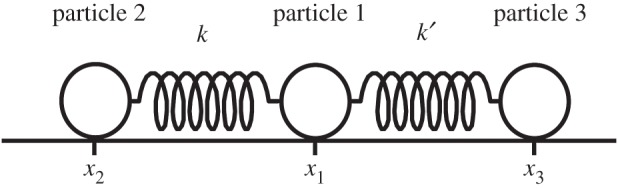
Three particles are connected with two springs. k and k′ are the constants of the two springs. x_i is a position of the particle i.

First, let us take k=10 and k′=0 in order to discuss the simple case of the two-body system. Then, the trajectory becomes the same as the analytical solution, i.e. the usual periodic vibration of a spring (figure 4a). Second, we take k=9.75, k′=0.25 for the three-body system. In addition, there is an analytical solution in this special case (see appendix A). The resultant trajectory of particle 1 is obtained as shown in figure 4b.

Figure 4.

Trajectories of the coordinates of particle 1 (x₁); the initial equilibrium positions of particles 1, 2 and 3 are 0, −5 and 5, respectively. Initial velocities are all 0. After moving particle 1 to position x₁=1, the simulation was started. The time step was Δt=0.01. The simulation was performed for 4000 steps under the relations V _n+1=V _n+FΔt/m, where V _n represents the velocity of the respective particles at the nth time step and F is the force exerted on the respective particle by the springs between two particles (1 & 2 and 1 & 3) with the respective spring constants. (a) Trajectory in the two-body system: k=10 and k′=0; (b) trajectory in the three-body system: k=9.75 and k′=0.75.

We define two quantities p and q to discuss the complexity of the one-dimensional three-body system.

The quantity p is given by the ratio of spring constants as

4.1

Obviously, if p=0 or 1, then the trajectories of the two-body system appear. Thus, the parameter p encodes the information of the experimental situation (context) whether it is a two- or three-body system. This parameter reflects the basic features of the context. (Context is determined by the pair of parameters k and k′.) In our simulations, the values of parameters k and k′ will be fixed. And we shall simply speak about contexts C₂₃: both springs are present, and C_i: only the ith spring is present. These are the analogues of the corresponding contexts for the two-slit experiment: only one slit is open or both slits are open. These are also the analogues of the corresponding contexts for lactose–glucose metabolism in E. coli bacteria (figure 2).

Another quantity q is the probability of particle 1 being in range of x₁>a, where, just to be specific in the numerical simulation, we chose a=0.2,a=0.8. Formally, q is defined as

4.2

Here, n is the number of time steps of particle 1 existing at x₁>a, and N is the number of time steps of the entire simulation.

Figure 5a shows the probabilities (q) of particle 1 being in a certain range of x₁ within a certain time period T=40 under three-body interactions by changing the contributions of the two springs by p=k/(k+k′)(0≤p≤1), compared with the probabilities under of the respective independent two-body interactions (p=1 or p=0), which is solved analytically.

Figure 5.

Probability q depends on the contribution of the two spring constants by p compared with the case of each spring working independently. The simulation conditions are described in the legend to figure 3. The probability depending on the ratio of p was calculated as the ratio of the number of time steps when particle 1 exists in the range of x₁>0.2 or x₁>0.8 during the total simulation time N=4000 time steps (time step is 0.01), during which particle 1 should exist somewhere between positions 1 and −0.35 depending on the ratio of the spring constants, as shown in figure 4a,b. (a) Probabilities of particle 1 being in the ranges of x₁>0.2 and x₁>0.8 and (b) intensity of violation of the FTP.

We can practically repeat the discussion on lactose–glucose interference. We can say that particle 1 ‘recognizes’ particles 2, 3 (as a bacterium recognizes molecules of lactose and glucose). The ‘response’ of 1 is + if it is in the range x₁>a (a=0.2,a=0.8 in our numerical simulation) and − in the opposite case. Our numerical simulation demonstrated (figure 5b) that the interaction of particle 1 and particles 2, 3 leads to violation of the classical FTP:

4.3

Probabilities P(2),P(3) are determined by the contributions of the springs: P(2)=p,P(3)=1−p. Probabilities P(+),P(+|2),P(+|3) of particle 1 being in the range x₁>a (the q parameter in the above consideration) are determined by experimental contexts C₂₃,C₂,C₃. Interference of the interactions of particle 1 with particles 2,3 is represented as the appearance of the interference term perturbing the classical FTP:

4.4

The results of the numerical simulation for λ are presented in §4b.

Similar to the two-slit experiment (2.4), (2.5) and the Lac operon activation experiment (3.3), (3.4), we can represent this multi-contextual setting by using the quantum formalism. Contexts C₂₃,C₂,C₃ are represented by the states |ψ〉,|2〉,|3〉. Then

4.5

where the state |i〉 represents context C_i,i=2,3, and

4.6

where |±〉 are eigenvalues of the ‘being in the range x₁>a observable.’ Finally, we once again use Born's rule (2.6) to obtain the quantum-like FTP (4.4).

(b). Quantum-like interference coefficient for interactions in three-body systems

By numerical simulation, we can estimate the values of conditional probabilities:

4.7

We change the value of the spring constants as follows:

4.8

Then we have the probabilities (p_i,q_i) for each pair of spring constants. We can obtain the value of λ_i in equation (3.2) by using numerical simulation (figure 6).

Figure 6.

Interference coefficient λ for the range of {x>0.8} and {x>0.2}.

We show the value of λ for the range of {x>0.8}, and λ for the range of {x>0.2}. Here, we fixed the k+k′=10. As we can see, the interference coefficient λ takes a negative value. Thus, the interference is destructive. This coefficient exceeds −1, when p is around zero or 1. Figure 6 shows the plot with respect to p in [0.05,0.95]. There exists the λ whose value exceeds −1. Thus, the quantum-like representation (4.5), (4.6) is idealized and one has to proceed with POVMs or in the framework of general adaptive dynamics [24].

Also, for p in the middle range (around 0.5), the intensity of interference seems to be very weak, since λ takes values around zero. We interpret the case k=k′ as the classical mixture.

5. Conclusion

We identified the interference term for the three-body system, the simplest complex system. We proceeded in the same way as in quantum physics (the two-slit experiment [1]) and quantum-like modelling in molecular biology (E. coli diauxic growth [23]). The interference term depends on the spring's stiffness. The results show that the classical three-body system which has more than two interactions at the same time on at least one member of the system can exhibit non-classical probabilistic features, thus it can be treated as the NKP system. Again, as well as in the case of the two-slit experiment and E. coli diauxic growth, violation of the FTP can be modelled by using the Hilbert state formalism of quantum theory: state superposition and Born's rule.

This classical three-body system, which provides a metaphor for quantum probabilistic behaviour, is important to justify the use of the quantum formalism in biology, where stochasticity is a consequence of functioning of a complex network of interactions between molecules and cells. Now it is clear that classical interactions between subsystems of a complex system can lead to non-classical (quantum-like) probabilistic features. This should stimulate further applications of quantum-like methods in biology.

Appendix A. Analytical solution of the one-dimensional three-body problem

Here, we use the notation shown in §4a. Newton's equation of motion is written in matrix form:

A 1

A 2

Here, we rewrite the above equation with the new coordinates y₁=x₁, y₂=x₂+5 and y₃=x₃−5 as follows:

A 3

A 4

The 3×3 matrix in equation (A 4) is diagonalizable if k≠k′. Therefore, we can rewrite equation (A 4) as

A 5

Here, α_i is an eigenvalue of the matrix. Let (z₁,z₂,z₃)^t be the A(y₁,y₂,y₃)^t, then we have simple equations:

A 6

Therefore, we can obtain solutions of with constants Z_i, then the solution y_i as the linear combination of z_j:

A 7

Thus, we can have the analytical solution of x_i in the settings of figure 3. The eigenvalues α_i determine the periodicity of the orbits. However, the orbit is not periodic, but chaotic in general.

Authors' contributions

M.A. designed the study and analysed the data; A.K. wrote the manuscript and participated in data analysis; M.O. coordinated the study and helped in the design/analysis of the study and manuscript preparation; Y.T. wrote the manuscript, participated in the design of the study and participated in data analysis; I.Y. carried out the simulation study, designed the study and analysed the data.

Competing interests

We declare we have no competing interests.

Funding

A.K. was partially supported by a grant from the programme Mathematical Modeling of Complex Hierarchic Systems of the Faculty of Technology, Linnaeus University, and a QBIC-grant from the Tokyo University of Science.

References

- 1.Feynman RP. 1951. The concept of probability in quantum mechanics. In Proc. of the 2nd Berkeley Symposium on Mathematical Statistics and Probability, Berkeley, CA, 31 July–12 August 1950, pp. 533–541. Berkeley, CA: University of California Press.
- 2.Kolmogorov AN. 1956. Foundations of the theory of probability. New York, NY: Chelsea Publishing Company. [Google Scholar]
- 3.Khrennikov AY. 2010. Ubiquitous quantum structures: from psychology to finances. Berlin, Germany: Springer. [Google Scholar]
- 4.Cheon T, Takahashi T. 2010. Interference and inequality in quantum decision theory. Phys. Lett. A 375, 100–104. ( 10.1016/j.physleta.2010.10.063) [DOI] [Google Scholar]
- 5.Takahashi T, Cheon T. 2012. A nonlinear neural population coding theory of quantum cognition and decision making. World J. Neurosci. 2, 183–186. ( 10.4236/wjns.2012.24028) [DOI] [Google Scholar]
- 6.Haven E. 2008. Private information and the ‘information function’: a survey of possible uses. Theory Decis. 64, 193–228. ( 10.1007/s11238-007-9054-2) [DOI] [Google Scholar]
- 7.Ishio H, Haven E. 2009. Information in asset pricing: a wave function approach. Ann. Phys. 18, 33–44. ( 10.1002/andp.200810333) [DOI] [Google Scholar]
- 8.Accardi L, Ohya M. 1999. Compound channels, transition expectations, and liftings. Appl. Math. Optim. 39, 33–59. ( 10.1007/s002459900097) [DOI] [Google Scholar]
- 9.Plotnitsky A. 2014. Are quantum-mechanical-like models possible, or necessary, outside quantum physics? Phys. Scr. 2014, 014011 ( 10.1088/0031-8949/2014/T163/014011) [DOI] [Google Scholar]
- 10.Bell JS. 1964. On the Einstein-Podolsky-Rosen paradox. Physics 1, 195–200. [Google Scholar]
- 11.Accardi L. 1997. Urne e camaleonti: dialogo sulla realtà, le leggi del caso e l'interpretazione della teoria quantistica. Rome, Italy: Il Saggiatore; [In Italian.] [Google Scholar]
- 12.Asano M, Hashimoto T, Khrennikov A, Ohya M, Tanaka Y. 2014. Violation of contextual generalization of the Leggett–Garg inequality for recognition of ambiguous figures. Phys. Scr. 2014, 014006 ( 10.1088/0031-8949/2014/T163/014006) [DOI] [Google Scholar]
- 13.Khrennikov A, Haven E. 2009. The importance of probability interference in social science: rationale and experiment. J. Math. Psychol. 53, 378–388. ( 10.1016/j.jmp.2009.01.007) [DOI] [Google Scholar]
- 14.Asano M, Basieva I, Khrennikov A, Ohya M, Tanaka Y, Yamato I. 2015. Quantum information biology: from information interpretation of quantum mechanics to applications in molecular biology and cognitive psychology. Found. Phys. 45, 1362–1378. ( 10.1007/s10701-015-9929-y) [DOI] [Google Scholar]
- 15.Busemeyer JR, Bruza PD. 2012. Quantum models of cognition and decision. Cambridge, UK: Cambridge University Press. [Google Scholar]
- 16.Ezhov AA, Berman GP. 2003. Introduction to quantum neural technologies. Paramus, NJ: Rinton Press Inc. [Google Scholar]
- 17.Bagarello F. 2012. Quantum dynamics for classical systems: with applications of the number operator. New York, NY: John Wiley & Sons. [Google Scholar]
- 18.Asano M, Khrennikov A, Ohya M, Tanaka Y, Yamato I. 2015. Quantum adaptivity in biology: from genetics to cognition. Berlin, Germany: Springer. [Google Scholar]
- 19.Accardi L, Imafuku K, Regoli M. 2002. On the EPR-Chameleon experiment. Infin. Dimens. Anal. Quantum. Probab. Relat. Top. 5, 1–20. ( 10.1142/S0219025702000687) [DOI] [Google Scholar]
- 20.Ohya M, Volovich I. 2011. Mathematical foundations of quantum information and computation and its applications to nano- and bio-systems. Berlin, Germany: Springer. [Google Scholar]
- 21.Asano M, Basieva I, Khrennikov A, Ohya M, Tanaka Y, Yamato I. 2012. Quantum-like model of diauxie in Escherichia coli: operational description of precultivation effect. J. Theoret. Biol. 314, 130–137. ( 10.1016/j.jtbi.2012.08.022) [DOI] [PubMed] [Google Scholar]
- 22.Khrennikov AY, Loubenets ER. 2004. On relations between probabilities under quantum and classical measurements. Found. Phys. 34, 689–704. ( 10.1023/B:FOOP.0000019631.84010.a6) [DOI] [Google Scholar]
- 23.Basieva I, Khrennikov A, Ohya M, Yamato I. 2011. Quantum-like interference effect in gene expression: glucose–lactose destructive interference. Syst. Synth. Biol. 5, 59–68. ( 10.1007/s11693-011-9081-8) [DOI] [PMC free article] [PubMed] [Google Scholar]
- 24.Asano M, Basieva I, Khrennikov A, Ohya M, Yamato I. 2013. Non-Kolmogorovian approach to the context-dependent systems breaking the classical probability law. Found. Phys. 43, 895–911. ( 10.1007/s10701-013-9725-5) [DOI] [Google Scholar]