Field Data and Numerical Modeling: A Multiple Lines of Evidence Approach for Assessing Vapor Intrusion Exposure Risks

Abstract

USEPA recommends a multiple lines of evidence approach to make informed decisions at vapor intrusion sites because the vapor intrusion pathway is notoriously difficult to characterize. Our study uses this approach by incorporating groundwater, soil gas, indoor air field measurements and numerical models to evaluate vapor intrusion exposure risks in a Metro-Boston neighborhood known to exhibit lower than anticipated indoor air concentrations based on groundwater concentrations. We collected and evaluated five rounds of field sampling data over the period of one year. Field data results show a steep gradient in soil gas concentrations near the groundwater surface; however as the depth decreases, soil gas concentration gradients also decrease. Together, the field data and the numerical model results suggest that a subsurface feature is limiting vapor transport into indoor air spaces at the study site and that groundwater concentrations are not appropriate indicators of vapor intrusion exposure risks in this neighborhood. This research also reveals the importance of including relevant physical models when evaluating vapor intrusion exposure risks using the multiple lines of evidence approach. Overall, the findings provide insight about how the multiple lines of evidence approach can be used to inform decisions by using field data collected using regulatory-relevant sampling techniques, and a well-established 3-D vapor intrusion model.

1. Introduction

Vapor intrusion involves indoor air contamination resulting from chemical volatilization in the subsurface beneath the building. Because of the complexities associated with characterizing the vapor intrusion pathway, the United States of Environmental Protection Agency (USEPA) recommends a “multiple lines of evidence approach” when making decisions about how to assess vapor intrusion exposure risks (USEPA, 2015a). The multiple lines of evidence approach uses field data, modeling and other pertinent site information to assess vapor intrusion exposure risks. However, approaches for integrating the various sources of data are not well established. To gain a better understanding of the implications of various approaches, the authors conducted a vapor intrusion investigation in a neighborhood with a well-characterized subsurface contamination plume and compared field data results with numerical modeling results.

USEPA issued two different documents that provide technical guidance on how to interpret and evaluate vapor intrusion data; one document is primarily related to field data, (USEPA, 2012a) and the other report results of a 3-D model used to evaluate various conceptual site models (USEPA, 2012b). However, the comparison of high-quality, temporally-correlated field data with model predictions remains a critical need within the vapor intrusion community (Turczynowicz and Robinson, 2007; Yao et al., 2013a).

Using a systematic comparison of the model predictions and field measurements, this paper represents one of the first attempts to report the results of a multiple lines of evidence approach using a 3-D vapor intrusion model and field data collected using regulatory-relevant sampling techniques at a real-world vapor intrusion site. The data show that in order for multiple lines of evidence to provide meaningful information about vapor intrusion exposure risks, relevant physical models must be included and evaluated.

Results discussed herein provide scientific insight about the multiple lines of evidence approach, and also are grounded in the realistic constraints that a “living” site poses. This study intentionally does not investigate new or emerging characterization techniques; rather its main purpose is to provide novel insights about comparisons between data collected using common field sampling techniques and results of a well-established vapor intrusion numerical models. Accordingly, the findings summarized herein are timely and relevant to the broad vapor intrusion community including researchers, practitioners and regulatory agency staff.

2. Methods and Materials

2.1. Site Description

The field study site is the neighborhood adjacent to a former chemical handling facility where bulk tetrachloroethylene (PCE) (and other chlorinated solvents) was transported for offsite use. Over the period of time that the site operated (1955-2002), the soil and groundwater became contaminated. Groundwater contamination (chlorinated VOCs, predominantly PCE with little to no evidence of degradation) migrated northeast (GEI, 2009). The neighborhood consists of residential and commercial properties, as well as an elementary school. The site had been involved in regulatory action for several years, dating back to the mid-2000s. As part of the ongoing regulatory activities mandated by the Massachusetts Department of Environmental Protection (MassDEP), the vapor intrusion pathway was evaluated. A number of vapor intrusion mitigation systems had been installed at buildings throughout the neighborhood, including the school, and many residences. In accordance with MassDEP regulation, ongoing monitoring was conducted to evaluate other buildings that might require mitigation and whether current mitigation systems are performing adequately (GEI, 2009). This study was conducted to gain additional insight about the vapor intrusion pathway at the site and to investigate the use of a 3-D vapor intrusion model to inform and interpret vapor intrusion data sets.

The field study site is schematically shown on Fig. 1. The study included three properties A, B and C. The selection of properties was made based on proximity to the source of contamination and the property owners' (and property tenants') willingness to participate in the study. Each property owner allowed research personnel access to his or her outdoor and indoor premises on a repeated basis from 2010 through 2012. Throughout the field study, members of the research team discussed results and the associated vapor intrusions risks with the property owners, and MassDEP.

Fig. 1. Site Map Showing Sampling Location.

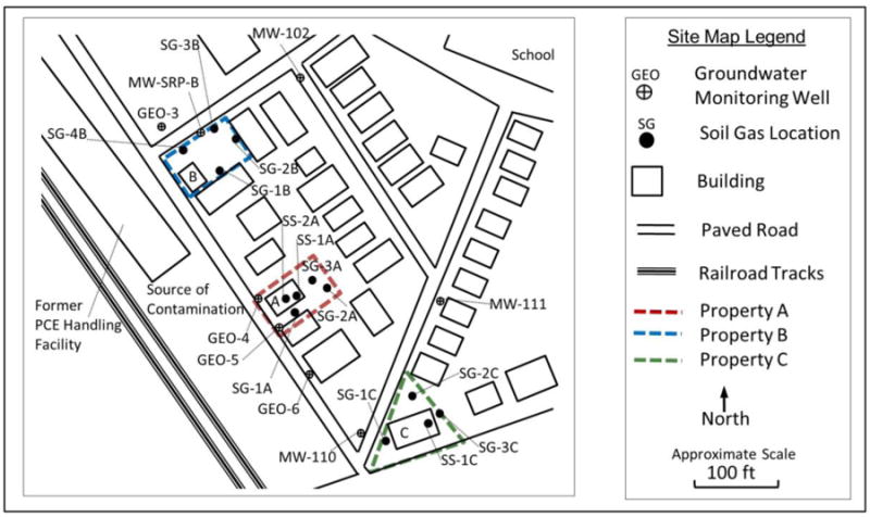
(SG: Soil gas borings; MW and GEO: Monitoring Well)

Property A includes a three story multi-family home (basement depth approximately 5.5 feet bgs) with a paved patio (approximately 32 ft by 23 ft) and a grassy area (42 ft by 29 ft) northwest of the home. Property B includes an open space grassy field (approximately 50 ft by 50 ft) with a three-story multifamily home is located in the southwest corner. Property C is a slab-on-grade building that was used for commercial purposes. The entire surface area for Property C was asphalt paved (maximum dimensions were approximately 58 ft by 93 ft). The contaminant source was located to the west of these properties.

All three of these properties were inhabited and in use throughout the study. Accordingly, like most vapor intrusion sites across the country, each property had certain limitations that could not be overcome. For instance, Property B had an active vapor intrusion mitigation system and the basement floor and walls had been sealed prior to this research. Therefore, we did not specifically evaluate indoor air concentrations from this property; however vapor intrusion exposure risks were evaluated by using soil gas and groundwater data, along with 3D modeling. Other specific circumstances are noted in Table 1.

Table 1. Sample Media and Collection Locations.

Property	Soil Gas			Indoor Air	Groundwater4
	Location	ft (bgs)	Surface Cover
A	SG-1A	3, 5, 7	Pavement	Basement1 First Floor1 Outside	GEO-3 GEO-4 GEO-5 GEO-6 MW-102 MW-110 MW-111 MW-SRP-B
	SG-2A	3, 5	Grass
	SG-3A	3, 5	Pavement
	SS-1A	1.75	Concrete
	SS-2A	0.5	Concrete
B	SG-1B	3, 5, 7	Grass	Not included in this study2
	SG-2B	3, 5, 7	Grass
	SG-3B	3, 5, 7	Grass
	SG-4B	3, 5, 7	Pavement
C	SG-1C	3, 5	Pavement	First Floor3 Outside
	SG-2C	5, 7	Pavement
	SG-3C	3, 5, 7	Pavement
	SS-1C	5	Concrete

Notes: bgs: below ground surface

¹The indoor air on the first floor was only sampled during the first event due to access restrictions by the property owner. Beginning with the second sampling event, only two basement indoor samples were collected.

²Soil gas and groundwater data were included in the analysis of Property B. However, since this property had an active vapor intrusion mitigation system and the basement floor and walls had been sealed prior to this research, indoor air data is not included herein. In addition, during sampling activities, sewer gas was determined to be the source of elevated PCE concentrations detected in the indoor air for Property B. Following the sewer connection being sealed, the PCE concentration detected in indoor air decreased significantly. Pennell et al. (2013) discuss the sewer-to-indoor air pathway for Property B.

³The building was a slab on grade construction, so there was no basement.

⁴Groundwater samples were collected from each of these wells. All of the wells, except, MW-SRP-B had been previously installed at the site as part of on-going regulatory action. MW-SRP-B was installed as part of this study and was located within Property B's boundary.

2.2. Multiple Lines of Evidence Approach

As a first step in the multiple lines of evidence approach, USEPA recommends to review site historical data and develop a site conceptual model. Then, risk-based site screening using empirically derived attenuation factors (α) is often performed (USEPA 2015a).

$${\alpha }_i=\frac{C_{\mathit{\text{indoor air}}}}{C_{\mathit{\text{location}},i}}$$ (1)

C_{indoor air} is indoor air concentration and C_{location, i} is the gas-phase concentration at a given (“i”) location. USEPA (2015a) recommends “screening” attenuation factors based on the location “i”. For instance, if the denominator is the chemical concentration in groundwater, then the term α_groundwater is used. If the denominator is the chemical concentration in the subslab, then the term α_subslab is used.

Where:

$${\alpha }_{\mathit{\text{groundwater}}}=\frac{C_{\mathit{\text{indoor air}}}}{C_{\mathit{\text{gas}}-\mathit{\text{phase groundwater}}}}=\frac{C_{\mathit{\text{indoor air}}}}{C_{\mathit{\text{groundwater}}}\times H}$$ (2)

Note: H is Henry's law constant (dimensionless)

$${\alpha }_{\mathit{\text{subslab}}}=\frac{C_{\mathit{\text{indoor air}}}}{C_{\mathit{\text{subslab}}}}$$ (3)

It is worth noting that higher attenuation factors suggest less attenuation. For instance, α_groundwater=10^-3 indicates three-orders of magnitude lower concentration in indoor air as compared to the groundwater (source) concentration. Whereas, α_groundwater=10^-6 corresponds to six-orders of magnitude lower concentration in indoor air as compared to the source concentration.

Comparison of predicted indoor air concentrations with risk-based guideline concentrations provides rationale for measuring indoor air concentrations (USEPA 2015a). For instance, if screening indicates the potential for vapor intrusion (e.g. an indoor air concentration that is calculated to be greater than the regulatory indoor air target), then indoor air samples are often collected; however, because consumer products contain many of the same compounds as those that are a concern for vapor intrusion (USEPA, 2011), indoor air samples often provide misleading information about the relative contribution of vapors from the subsurface source. To overcome limitations of indoor air concentration data, practitioners often install subslab (beneath the building foundation) and/or soil gas vapor sampling points located outside of the building footprint.

As an initial step, we reviewed historic field data for the site and developed a site conceptual model. Then, we collected indoor air and groundwater samples and compared them to our vapor intrusion screening assessment (Line of Evidence 1). As subsequent lines of evidence, we collected and evaluated soil gas data (Line of Evidence 2), and evaluated the field data using computational models (Line of Evidence 3). Finally, we created a revised site conceptual model based on the field data and numerical model results.

2.3. Field Sampling

A total of fourteen (14) soil borings were advanced as part of this field study. Fig. 1 shows the sampling locations. Ten (10) borings (SG-1A, SG-2A, SG-3A, SG-1B, SG-2B, SG-3B, SG-4B, SG-1C, SG-2C, and SG-3C) were completed as exterior soil gas sampling points nested at multiple depths in the yards and parking areas of the three properties included in the study (Properties A, B and C). One boring (MW-SRP-B) was completed as a 1″-dia monitoring well (15 ft deep), located in the yard of Property B. Table 1 summarizes the sample locations included in the study.

All soil gas sampling points were installed and sampled in accordance with recommended procedures (NYDOH, 2006). Field personnel examined soil borings during sample installation activities to gain insight about the site's geology. When possible, a Geoprobe® was used to advance the soil borings, and soil cores were collected in 4-foot acetate sleeves. Soil types were generalized based on field observations, coupled with sieve analysis of select samples. Generally speaking, the soil geology was consistent with the observations across the rest of the site, as previously reported by the environmental consultant for the site (GEI, 2009). The soil geology was surprisingly consistent, including two primary soil types: an upper unit (0-4 ft bgs) consisting of urban fill; and, a lower unit consisting a dense, stiff, sandy clay loam (4-8 ft bgs).

2.4. Chemical analysis

Groundwater, air and soil gas samples were collected every 2-3 months over a period of 12 months for a total of 5 sampling events. All samples (groundwater, indoor air and soil gas) for a given property were collected within 48 hours for each of the 5 sampling events. All samples (groundwater, air, and soil gas) were analyzed for selected VOCs based on detections reported during historical site sampling activities: PCE; Trichloroethylene (TCE); 1, 2, Dichloroethane (DCA); Trichloroethane (TCA); and Carbon tetrachloride (CCl₄).

2.4.1. Groundwater Sampling

Groundwater was collected from seven existing monitoring wells (GEO-3, GEO-4, GEO-5, GEO-6, MW-102, MW-110, and MW-111) and one well installed as part of this research (MW-SRP-B). Depth to groundwater was measured, and the groundwater level was compared to well construction details to ensure that the well screen was not submerged, as required for no-purge sampling. All groundwater samples were collected with disposable bailers using the no-purge method (API, 2000). Although the no-purge method is often limited to petroleum hydrocarbon sites, the nature of this field study posed limits on hazardous waste generation (including purge water) and also the amount of time to access each property. Therefore, the no-purge method was deemed the only possible method for sampling. Samples were shipped on ice to Columbia Analytical Services and analyzed for selected VOCs using EPA Method SW8260.

2.4.2. Air and Soil Gas Sampling

Air samples were collected inside and outside of each property for 24-hours using 6-L certified summa canisters and shipped overnight to Columbia Analytical Services for TO-15 analysis. Prior to sampling, research team members met with the residents to discuss the sampling process and to survey and remove possible indoor sources of VOCs from the home.

Soil gas samples were collected as grab samples over a period of 10 minutes using 1-L certified summa canisters. Summa canisters (both 1L and 6L) were certified “clean” and the flow controllers were certified by the laboratory prior to field sampling. All data reported are from canisters with acceptable vacuums upon receipt at the laboratory. Laboratory sample preparation and analysis was conducted by a National Environmental Laboratory Accreditation Conference-certified laboratory (Columbia Analytical Services). Analyses were compliant with USEPA Method TO-15 (Volatile Organic Compounds in Air Analyzed by Gas Chromatography/Mass Spectrometry) and the laboratory's standard operating procedures that define requirements for calibration and acceptable results for QC parameters. Detection limits are all below risk-based comparative values.

2.5. Computational Modeling

In general, most vapor intrusion models are 1-D screening tools. The most widely employed screening model is the Johnson and Ettinger, or J&E model (Johnson and Ettlnger, 1991), which has been incorporated into a spreadsheet program by USEPA (2004). The J&E model predicts attenuation factors based on user inputs; however it does not incorporate information about soil gas concentrations and therefore is not useful in interpreting the type of data typically collected during vapor intrusion investigations. 3-D models provide information about the soil gas concentrations throughout the subsurface, as well as the calculated attenuation factor, but are not widely available in practice settings due to lack of practitioners and regulations who have access to and are trained using 3D vapor intrusion models. In addition, there is a critical need for field data sets to be compared to 3D model results. This research incorporated 3D model simulations to investigate soil gas concentration profiles. For comparison purposes, results from USEPA's version of J&E model (groundwater contamination advanced model, GW-ADV-Feb04.xls (USEPA, 2004)) are also reported.

The 3-D model simulations included herein were conducted using a commercially available software, Comsol Multiphysics®. The modeling approach has already been extensively described (Bozkurt et al., 2009; Pennell et al., 2009; Yao et al., 2011). The model incorporated a generic single building (10 m × 10 m) with a basement (1.67 m deep) located in the center of an open field. A generic building geometry was used to allow comparisons between the 1-D J&E model and the 3D model. The model was exercised assuming a typical disturbance pressures (-5 Pa) at the perimeter crack (5mm wide) around the entire floor of the basement. Groundwater (located at 11ft bgs and 13 ft bgs) was assumed to be the vapor intrusion source. Various geological characteristics, including soil type, depth and thickness of the soil layers and moisture content of the soil were investigated and modeled. For this research, steady state model solutions are reported; however, separate ongoing research is considering transient effects. Table 2 summarizes the model equations.

Table 2. Model Equations.

Equation 1: Soil=gas continuity $q=\frac{-K\rho }{\mu }\nabla \varphi$ $\varphi =gz+\underset{Po}{\overset{P}{\int }}\frac{dP}{\rho }$	Where: q = gas velocity (L/t) K = intrinsic permeability (L2) ρ = density of soil gas (M/L3) μ = dynamic viscosity of soil gas (M/L/t) g = gravitational acceleration (L/t2) P = pressure of soil gas (M/L/t2) z = elevation (L) Note: Equation 1 is valid for gas flow in soils where slip flow is negligible (sand and gravels). For fine-grained materials, Darcy's Law (Equation 1) may underestimate flow.
Equation 2: Pressure drip across crack: $\mathrm{\Delta }{p}_{\mathit{\text{ck}}}=\frac{12Q_{\mathit{\text{ck}}}{\mu }_g{d}_{\mathit{\text{ck}}}}{w_{\mathit{\text{ck}}}^3}$ Note: Qck = QCER	Where: Δpck = Pressure drop across crack (assumes parallel plates)(M/L/t2) wck = width of crack (L) dck = length of crack through foundation depth (L) QCER = soil-gas flow rate into the characteristic entrance region (L3/t) Qck = soil-gas flow rate through crack into building (L3/t)
Equation 3: Chemical transport $J_{T,i}=q\cdot C_i-D_{\mathit{\text{eff}},i}^{\mathit{\text{gas}}}\nabla C_i$ $D_0^{\mathit{\text{eff}}}=D_g\frac{{\theta }_g^{10/3}}{{\theta }_t^2}+\frac{D_w}{{\mathrm{K}}_H}\frac{{\theta }_w^{10/3}}{{\theta }_t^2}$ Millington (1959)	Where: JT = Bulk mass flux of “i” (M/L2/t) C = Concentration of “i” in soil gas (M/L3) D0eff = Effective diffusivity coefficient on “i” in soil-gas phase (L2/t) Dg = Molecular diffusivity coefficient on “i” in air (L2/t) Dw = Molecular diffusivity coefficient on “i” in water (L2/t) KH = Air-water partition (Henry's) coefficient (unitless) θ = porosity; t = total, g = gas-filled, w = water-filled (L3/L3)
Equation 4: Indoor Air Concentration $C_{\mathit{\text{indoor}}}=\frac{A_{\mathit{\text{ck}}}{J}_T}{A_e{V}_b+Q_{\mathit{\text{ck}}}}$	Ack = Area of the crack for vapor entry (L2) Vb = Volume of enclosed indoor space (L3) Aer = Air exchange rate in building (1/t)

3. Results and Discussion

3.1.Summary of Field Data and Conceptual Site Model

Table 3 summarizes the maximum chemical concentrations detected during this field study for each sample medium. PCE and TCE were the constituents most often detected across all media. Other constituents were detected but their concentrations fluctuated during the various sampling events (data not shown). PCE was the only constituent that was routinely detected at all of the properties included in the study. In addition, PCE was detected at the highest concentration of all chemicals for all sample media. Analytical results from historical sampling activities (GEI 2009) indicated that PCE was not undergoing significant biodegradation and degradation byproducts were not typically observed at the site.

Table 3. Maximum Chemical Concentrations Detected During Field Study.

Sample Location	1,1,1 TCA	1,2 DCA	PCE	TCE	Carbon Tetrachloride	Vinyl Chloride	Media
GEO-3	17	<5	450	95	<5	<5	Groundwater (μg/L)
GEO-4	<100	<100	8100	100	<100	<100
GEO-5	110	<100	6100	190	<100	<100
GEO-6	<2	<2	25	7.2	<2	<2
MW-102	4.7	<2	74	6.5	<2	<2
MW-110	<2	<2	<2	<2	<2	<2
MW-111	<10	<10	880	12	<10	<10
MW-SRP-B	17	<2	300	84	<5	<5
Property A	17	<15	2300	0.38	<15	<15	Soil Gas (μg/m3)
Property B	360	<5.5	3900	410	<5.5	<5.5
Property C	<1.1	<1.1	2.8	<1.1	<0.40	<1.1
Property A	2.0	<0.42	300	7.7	<0.42	<0.42	Subslab (μg/m3)
Property B	NI	NI	NI	NI	NI	NI
Property C	<1.6	<1.6	28	2.3	0.86	<1.6
Property A	0.28	0.1	5.3	2.2	0.46	<0.04	Indoor Air (μg/m3)
Property B	*	*	*	*	*	*
Property C	0.5	0.073	2.7	0.32	0.86	<0.047
95th Percentile Background (EPA 2011)	3.4-28	<0.2	4.1-9.5	0.56-3.3	<1.1	<0.09	Indoor Air (μg/m3)
Residential Threshold Values (MassDEP 2011)	3.0	0.09	1.4	0.8	0.54	0.27	Indoor Air (μg/m3)
IA Target (VISL) (EPA 2015b)	5200	0.11	11	0.48	0.47	0.17	Indoor Air (μg/m3)
Subslab Target (VISL) (EPA 2015b)	170,000	3.6	360	16	16	5.6	Subslab (μg/m3)

Notes:

If a constituent was not detected during the study, the concentration is shown as less than the maximum detection limit for the study (e.g. <5). Underlined data exceed typical background concentrations in indoor air. Bolded data exceed threshold values set by MassDEP to be protective of human health. NI – Not installed. IA – Indoor Air.

^*Property B has an active vapor intrusion mitigation system and the basement had been sealed prior to this research. Sewer gas was determined to be the source of elevated PCE concentrations detected in the indoor air for Property B. Following the sewer connection being sealed, the PCE concentration detected in indoor air decreased significantly. Pennell et al. (2013) discuss the sewer-to-indoor air pathway for Property B.

Two conceptual site models were established as relevant for the initial representations of the vapor intrusion pathway at the site: 1) the classic conceptual model, a building located in the middle of an open field; and 2) a building surrounded by impervious material. Both of these conceptual models assumed groundwater was the source of chemical vapors in the subsurface.

In the classic conceptual model, soil gas is trapped beneath the building footprint. Outside the footprint, soil gas concentrations decrease as they approach the ground surface. Similarly, for the situation where a building is surrounded by an impervious surface, soil gas is trapped beneath the entire covered area. Outside the covered area, soil gas concentrations decrease as they approach the ground surface. These conceptual descriptions of vapor transport at the site guided the evaluation of each additional line of evidence and were informed by conceptual models available in the literature (USEPA 2012b; Pennell et al 2009; Bozkurt et al 2009).

3.2. Multiple Lines of Evidence

As discussed in section 2.2, we investigated three lines of evidence. First, we collected indoor air samples and groundwater samples, and compared them to our vapor intrusion screening assessment values (Line of Evidence 1, Section 3.2.1). Then, as subsequent lines of evidence, we collected and evaluated soil gas data (Line of Evidence 2, Section 3.2.2), and finally we evaluated the field data using computational models (Line of Evidence 3, Section 3.2.3). As a final result, we developed a revised conceptual site model.

3.2.1. Line of Evidence 1: Groundwater Screening and Indoor Air Concentration Measurements

As the first line of evidence, evaluating attenuation factors provides information about the propensity for vapor intrusion exposure risks at the site. For this line of evidence, we considered data that were previously collected as part of regulatory activities at the site (GEI 2009), as well as data specifically collected as part of this research. The results are summarized below and show relatively good agreement in terms of historical site trends.

3.2.1.1. Line of Evidence 1: Evaluation of Previously Collected Field Data

Based on prior field data collected as part of regulatory activities for the three properties included in this study (A, B and C), the attenuation factors ranged from approximately 10^-3 to 10^-6. These attenuation factors were calculated using historical groundwater and indoor air concentrations reported to MassDEP by the site consultant (GEI, 2009). The higher attenuation factor (10^-3) was detected in a Property B, which was later mitigated and the basement floor was sealed. Several years after mitigation, Pennell et al. (2013) reported evidence that a faulty sewer connection in Property B was a source for elevated PCE concentrations in the indoor air on the first floor during the field study included in this research. It is not known how long the sewer connection may have been influencing indoor air concentrations in that property. For Property A and Property C, the attenuation factors ranged from approximately 10^-5 to 10^-6, which are considerably lower and suggested vapor intrusion may not be a concern at these buildings; however, using the 0.001 screening value as the attenuation factor, “predicted” indoor air concentrations that are above MassDEP health risk levels. Since there is considerable research showing that indoor air concentrations vary temporally (e.g. Holton et al 2014), these data, by themselves, were not adequate to suggest there was not a “potential” for vapor intrusion exposure risks. Additional sampling was aimed at better understanding the potential for vapor intrusion exposure risks at the site (Lines of Evidence 1 and 2).

3.2.1.2. Line of Evidence 1: Evaluation of Data Collected as Part of “This” Study

Groundwater and indoor air samples were collected from locations across the site. Fig. 3 shows a comparison between measured indoor air concentrations and predicted indoor air concentrations using the USEPA screening attenuation factor of 0.001 (USEPA, 2015a) and groundwater concentrations that were detected in nearby wells. Fig. 4 shows the site-specific attenuation factors calculated based on indoor air concentrations detected at Properties A and C. Indoor air concentrations presented on these figures were limited to the lowest building level (the basement of Property A and the first-floor of Property C) and groundwater concentration data collected from individual monitoring wells located near the properties—Property A (GEO-4 and GEO-5) and Property C (MW-110, MW-111, GEO-6). Property B was excluded from this line of evidence because indoor air concentrations were known to be influenced by sewer gas entering the home (Pennell et al 2013). In should be noted that Property B is included in subsequent lines of evidence because sewer gas entering the home did not influence the soil gas concentrations (Line of Evidence 2) or modeling activities (Line of Evidence 3).

Fig. 3. Comparison of Screening Level “Predicted” and Measured Indoor Air Concentrations for Property A and Property C.

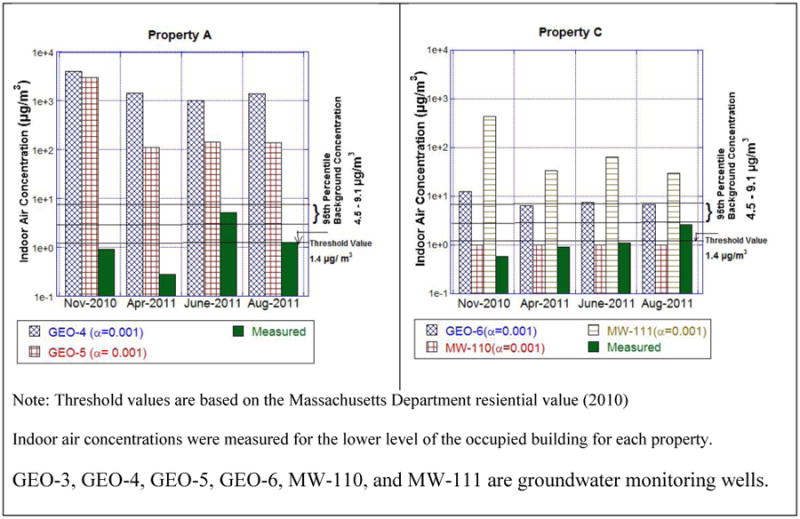
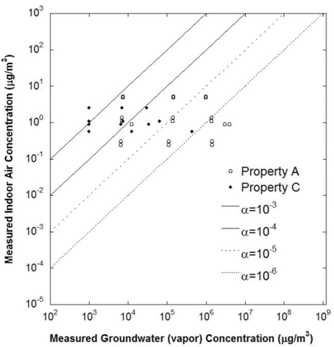
Fig. 4. Measured Groundwater (Vapor) Concentration and Attenuation Factors (α).

“Predicted” indoor air concentrations, calculated using the groundwater concentration data collected from individual monitoring wells located near the properties—Property A (GEO-4 and GEO-5) and Property C (MW-110, MW-111, GEO-6)—were above the MassDEP residential threshold values and typical indoor air background concentrations (MassDEP, 2011); however, nearly all of the measured indoor air concentrations detected for Property A and C were below the background (i.e. “typical”) levels, which suggests vapor intrusion exposure risks appeared low.

As shown on Fig. 4, despite that each of the groundwater monitoring locations were close to each of the respective properties (generally less than 100 feet) and were located in the same groundwater aquifer (shallow), groundwater concentrations varied and resulted in many orders of magnitude difference between the attenuation factors. This spatial variation is a challenge for many vapor intrusion investigations and is consistent with the analysis of other vapor intrusion field data (Yao et al., 2013b). The selection of appropriate monitoring wells for preliminary evaluation of vapor intrusion exposure risks is important, but not easily determined when designing a vapor intrusion investigation. Based on the data shown on Figs. 4 and 5, Properties A and C appear to have limited potential for vapor intrusion based on indoor air measurements, which is consistent with previous historical field sampling results (Section 3.2.1.1); however based on the known likelihood for indoor air concentrations to vary substantially with time (e.g. Holton et al 2014), additional evaluation of other field is warranted to fully consider whether a potential for vapor intrusion exposure risks is likely. To further evaluate the potential for exposure risks, soil gas concentrations were evaluated.

Fig. 5. Measured Soil Gas Concentrations as a Function of Sampling Depth.

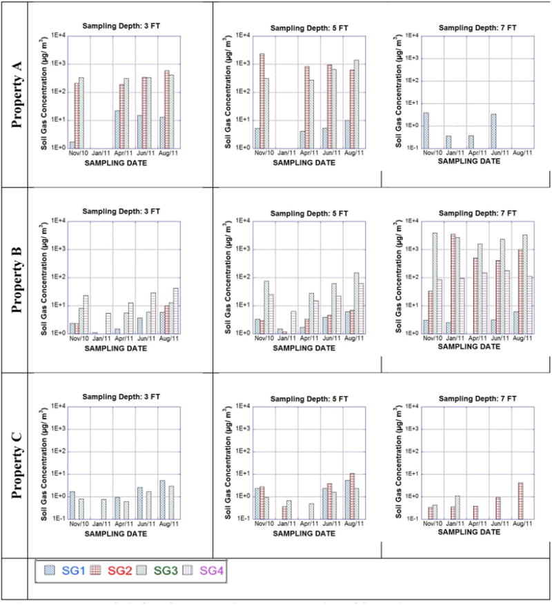
, Note: Blank space in measured column indicates no sample collected on that specific date. Property B was the only property with an SG-4 sampling location.

3.2.2. Line of Evidence 2: Soil Gas Concentrations

Soil gas concentration data provide another indication of potential for vapor intrusion exposure risks and are used as another line of evidence. Two different types of soil gas data are often collected: subslab soil gas samples (collected from beneath the building footprint); and, exterior soil gas samples (collected outside the building footprint).

Subslab Soil Gas Samples

Indoor air measurements at Property A suggest a low potential for vapor intrusion, but subslab concentrations were above screening levels. The recommended subslab to indoor air screening level attenuation factor (α_subslab) is 0.03 (USEPA, 2015a). Therefore, the screening level for subslab concentrations of PCE is 360 μg/m³, which assumes a target indoor air concentration of approximately 11 μg/m³ (USEPA 2015b). All sub-slab concentrations for Property A are below this level (ranging from 10-300 μg/m3). And, all five rounds of indoor air sampling confirmed that indoor air concentrations of PCE were at or below indoor air target concentrations. Subslab concentrations of PCE at Property C were low, similar in magnitude to the measured indoor air concentrations (See Table 3), and were inconsistent with the conceptual models shown in Fig 2. Exterior soil gas samples (discussed below) provided additional information to develop a revised conceptual model that could inform decisions at the site.

Fig. 2. Preliminary Conceptual Models for the Site.

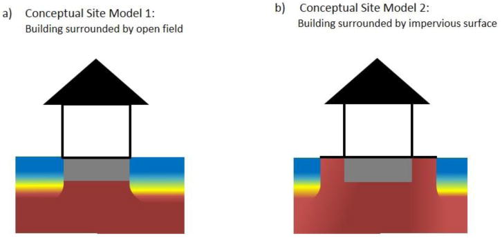
Notes: Red color indicates high concentration. Blue color represents low concentration.

Exterior Soil Gas Samples

The exterior soil gas data trends provide information about vapor attenuation throughout the subsurface (Fig. 5). The measured data show fluctuations over the course of the study; however temporal variations were slight. During the January, April and June sampling events, water-saturated conditions were observed in some of the shallow sampling locations. However, these conditions did not appear to affect results for subsequent events, which is likely related to the long time scales (i.e. many months) required for water infiltration to affect vapor transport in shallow soils. Shen et al. (2012) suggest the timescales for moisture content dynamics and the corresponding effects on vapor transport are disparate.

Considering the surface cover (Table 3) at each of the sampling locations and the conceptual models (Fig. 2a and Fig. 2b), one would expect the surface concentrations for SG-1 and SG-3 (Property A), SG-4 (Property B) and SG-1, SG-2 and SG-3 (Property C) to be fairly constant throughout the subsurface, since the paved surface may prevent upward diffusion (Fig. 2b). For all other locations, one would expect a decreasing trend as the sample depth decreases (Fig. 2a). Overall these “expected” trends are more or less observed (with the exception of SG-2 (Property A) and SG-4 (Property B)); however closer inspection of concentration gradients reveals that steep concentration gradients exist between the groundwater and the soil gas sampling depth at 7 ft bgs.

The data set for Property B was the most complete with regard to detected soil gas concentrations, number of soil gas sampling points, and geologic information; allowing for an in-depth analysis of spatial and temporal soil gas concentration trends, which are summarized in Fig. 6. As shown on Fig. 5, the data for Property A and Property C, although less complete, follow a similar trend and support the conclusions drawn from the Property B data.

Fig. 6. PCE Concentration Gradient for Soil Gas Locations at Property B.

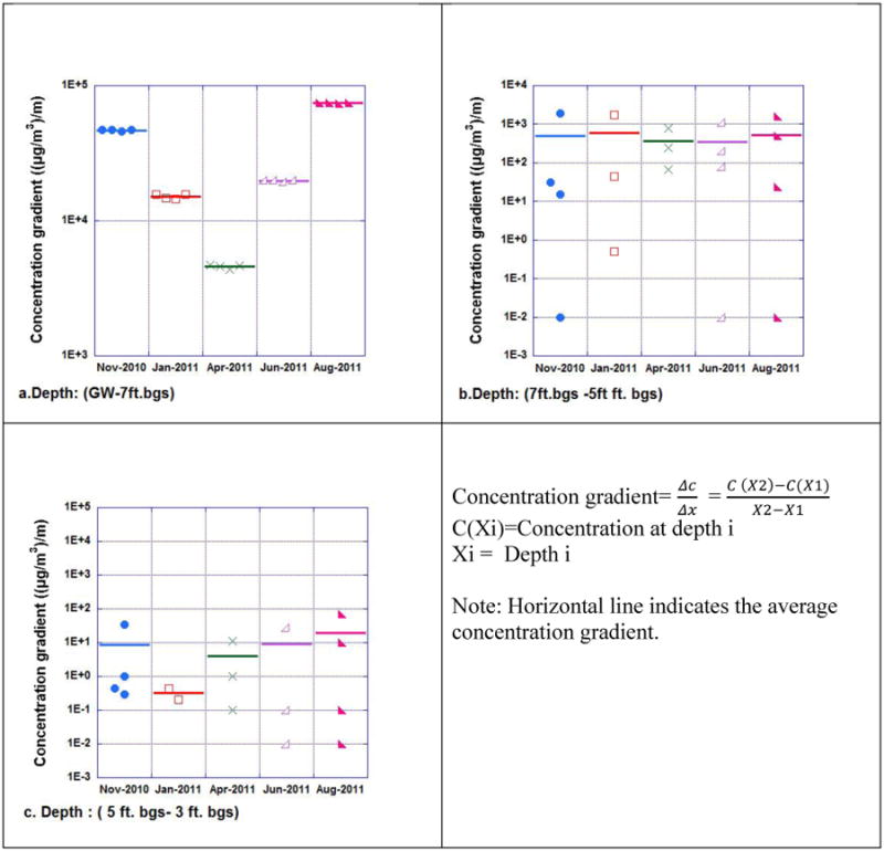
Fig. 6 illustrates that gradients in the deep soil gas locations (>7 feet) are orders of magnitude higher than the concentration gradients measured in shallow soils (<7 feet). Fig. 7a shows that concentration gradients are >1000 μg/m³/m for the soil zone located from the groundwater surface to 7 feet bgs, which is in contrast with shallow soils from 3 ft to 5 ft bgs (Fig. 7c), where the concentration gradient was <100μg/m³/m.

Fig. 7. Modeled and Measured Soil Gas Concentrations For Three Cases.

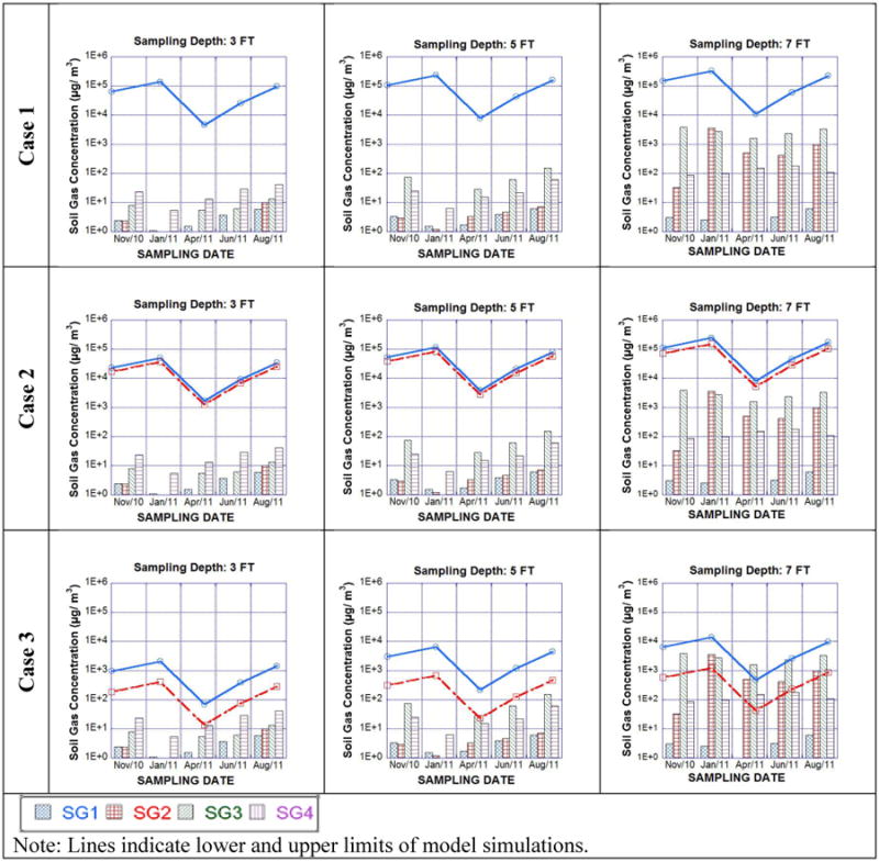
(For case 2, 3 there are two lines which show a range for variation of steady state concentration for different scenarios of each case)

As soil depth decreases, the concentration gradients also decrease, which disagrees with the theoretical understanding of vapor transport within a homogenous soil geology where concentration gradients would be linear across the soil depth. Based on the observed steep concentration gradient that exists at greater depths (>7 ft bgs), there appears to be a highly resistive subsurface feature that limits upward vapor transport. This resistive layer could be responsible for greater vapor attenuation and lower indoor air concentrations—which is consistent with the results shown in Fig. 4.

Inspection of the concentration gradients also reveals insight about spatial and temporal variations. Small spatial variation in soil gas concentration gradients were observed at depths >7 ft bgs, but slightly larger temporal variation (approximately 1-order of magnitude) across seasons. For shallower soils, larger spatial variation (>5 orders of magnitude) and smaller temporal variation (1.5 order of magnitude) are observed.

One possible explanation for increased attenuation in the subsurface is the capillary fringe, which is the zone of soil located immediately adjacent to the top of the water table. The effect of capillary fringe has been evaluated for vapor transport in laboratory settings and resulted in orders of magnitude increase in vapor attenuation (McCarthy and Johnson, 1993). Within the capillary zone, capillary forces draw water up into the soil pores and cause saturated soil conditions above the actual water table and reduces upward vapor transport. Trapped air that exists within the capillary zone prevents the soil from becoming fully saturated at the groundwater table surface; therefore, the effects of moisture content on vapor transport through the capillary zone has been approximated previously by Waitz et al. (1996) using moisture content estimates from water retention curve (e.g., van Genuchten (1980)). Bekele et al. (2014) reported elevated VOC concentrations (specifically TCE) in soil that was sandwiched between two high moisture zones. This observation also supports the observations reported herein where soil moisture is thought to have retarded VOC transport, trapping higher concentrations beneath highly resistive soil layers. Modeling efforts by Shen et al. 2012, 2013a, 2013b, and Moradi et al. 2015 also emphasize the importance of soil moisture when evaluating vapor intrusion exposure risks.

3.2.3. Line of Evidence 3: Interpret and Evaluate Field Data using Computational Modeling

The purpose of the modeling exercises was to investigate possible site characteristics that may provide a plausible explanation for the attenuation observed at the site. Modeling focused on predicting soil gas concentration data because soil gas concentrations are less prone to changes in building ventilation or chemical uses within the home. Further, indoor air concentrations were low across the entire site and did not lend themselves to further evaluation.

Model input values for the 3D model were based on field observations and relied on values recommended by USEPA (2004). Table 4 (below) describes the three cases that the models investigated. These cases were determined a priori and supported by site specific characteristics and field data. During the field study, the depth to groundwater varied in MW-B-SRP (located directly on Property B) from approximately 10 to 13 ft bgs; therefore, Case 3 was exercised for groundwater depths that ranged between 11-13 ft bgs. Case 1 and Case 2 were exercised for a groundwater depth of 11 ft bgs.

Table 4. Summary of the Scenarios.

Case	Description	α 3D	α J&E model
1	Homogenous geology for the two predominant soil types that were observed at the site (loamy sand and sandy clay)	4.5E-05 to 1.6E-04	1.9 E-04 to 8.8 E-04
2	Two-layer geological system with the top layer as a loamy sand and the bottom layer as a sandy clay.	3.3E-05 to 7 E-05	2.7 E-03 to 3.6 E-04
3	Three-layer geological system with the top layer as a loamy sand, middle layer as a sandy clay, and the bottom layer as a high moisture content (>90%) layer (conceptualized as the capillary fringe). Thickness of the capillary fringe varied from 1 ft to 2.5 ft, which corresponds to the soil types at the site.	1.6E-6 to 4.5E-6	4.00 E-06 to 1.00 E-05

The modeled attenuation factors are also shown in Table 4. It can be seen that adding a resistive layer in Case 3 increases attenuation by as much as nearly two order of magnitudes for both 3-D and J&E models. The attenuation factors demonstrate how site features can dramatically influence the potential for vapor intrusion exposure risks; however model simulations alone should not be used to make decisions at a site because models are well known to be subject to uncertainty related to model structure and environmental variability. Moradi et al (2015) highlights the effect of uncertainties on vapor intrusion exposure risk predictions and their results suggest that model predictions require the other lines of evidence to validate and inform about the likelihood of vapor intrusion exposure risks.

Fig. 7 depicts the measured and modeled soil gas concentrations for Property B. Spatially, a vertical concentration gradient was detected with the lowest concentrations detected at 3 ft bgs, and the greatest concentrations detected at 7 ft bgs. However, this gradient was not as steep as would be expected based on groundwater concentrations, and suggested that vapor attenuation was occurring deeper than the 7ft bgs sampling location. The inclusion of the high resistivity zone (conceptualized as the capillary fringe (Case 3)) results in an order of magnitude decrease in predicted attenuation factors and, importantly, improves model and field measurement agreement. Laterally, there was some variation in results for each soil gas sampling location, but overall the variations were less than one-order of magnitude.

Although the 3D model incorporated a capillary fringe layer, the highly resistive layer does not necessarily need to be the capillary fringe. It could be a thin fine-grained soil layer (i.e. clay and silt) located anywhere between groundwater and soil surface that can act as a barrier preventing upward migration of soil gas. It also could be a biologically reactive zone that prevents PCE from being transported upwards toward the surface prior to being degraded. It may also be a lens of “clean” water that overlies the groundwater surface; thereby reducing the source concentration that is estimated based on groundwater concentrations detected in monitoring wells. At this site, the measured groundwater concentrations did not provide a good indication of the vapor intrusion exposure risks (as measured by indoor air and soil gas concentrations). Regardless of the exact nature of the subsurface feature, the model established the location of the surface feature (which based on field data was deeper than 7 ft) and confirmed that the field observations were not consistent with the original conceptual models (Fig 2a/2b). Fig. 8 is an updated conceptual model.

Fig. 8. Conceptual Model Comparison.

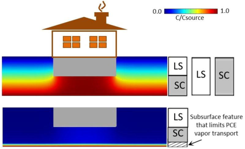
(top-classic, bottom-informed by this research). LS-loamy sand, SC-sandy clay

4. Conclusions

Characterizing vapor intrusion is difficult to accomplish because of sampling limitations and because field data do not easily follow predicted trends; however by systematically reviewing data and incorporating a numerical model to interpret field data observations using a multiple lines of evidence approach, decisions can be made about how to manage vapor intrusion exposure risks. Overwhelming evidence exists that a subsurface feature is present over much of the study area that limits upward vapor-phase diffusion of PCE. In addition, data suggest that the groundwater concentrations measured during this research, as well as the groundwater concentrations collected historically at the site as part of regulatory-driven activities, did not provide a good indication of vapor intrusion exposure risks (as estimated using the multiple lines of evidence approach). When vapor intrusion occurs in large communities where hundreds of homes are affected, our results indicate that relying on groundwater concentrations for assessing vapor intrusion exposure risks is not appropriate; and, deviations from classic conceptual vapor intrusion models should be anticipated. Incorporating physical models as part of multiple lines of evidence approach can inform conceptual models and improve risk management decisions.

While the collected data could not describe the exact nature of the subsurface “feature” that was limiting transport, the model did provide evidence that the subsurface feature would significantly alter the soil gas concentration profiles. Conceptually, the capillary fringe may be one possible explanation. If capillary fringe is the sole explanation, than soil gas concentrations at many vapor intrusion sites could be lower than expected based on the “classic” conceptual model. However, the results of this research did not provide enough information to support that claim. Rather, it suggests a need for additional research that evaluates high-quality, temporally-correlated field data with model predictions to investigate whether similar trends are present at other sites.

Future work involves incorporating a transient model to investigate soil gas and indoor air concentrations in response to groundwater seasonal behavior, and is also considering other possible processes like biodegradation, the impact of water lenses and atmospheric effects on soil gas transport.

Highlights.

• Multiple-lines-of-evidence can improve site-specific vapor intrusion risk assessments

• Combining field data and numerical model results improves site conceptual models

• Groundwater concentrations may not be predictive of vapor intrusion exposure risks

References

- API (American Petroleum Institute) No-Purge groundwater sampling: An Approach for Long Term Monitoring. Bulletin. 2000;12 [Google Scholar]
- Bekele DN, Naidu R, Chadalavada S. Influence of spatial and temporal variability of subsurface soil moisture and temperature on vapour intrusion. Atmospheric Environment. 2014;88:14–22. [Google Scholar]
- Bozkurt O, Pennell KG, Suuberg EM. Simulation of the vapor intrusion process for nonhomogeneous soils using a three-dimensional numerical model. Ground Water Monitoring & Remediation. 2009;29:92–104. doi: 10.1111/j.1745-6592.2008.01218.x. [DOI] [PMC free article] [PubMed] [Google Scholar]
- Holton C, Luo H, Dahlen P, Gorder K, Johnson PC. Temporal variability in indoor air concentrations under natural conditions in a house overlying a dilute chlorinated solvent plume. Environmental Science and Technology. 2013;47:13347–13354. doi: 10.1021/es4024767. [DOI] [PubMed] [Google Scholar]
- GEI (GEI Consultants) Immediate response action completion report and remedial monitoring report no 11 (RTN 3-23246) 2009 [Google Scholar]
- Johnson PC, Ettinger RA. Heuristic Model for Predicting the Intrusion Rate of Contaminant Vapors into Buildings. Environmental Science and Technology. 1991;25(8):1445–1452. [Google Scholar]
- MassDEP (Massachusetts Department of Environmental Protection) Interim final vapor intrusion guidance. 2011 WSC#11-435. [Google Scholar]
- McCarthy KA, Johnson RL. Transport of volatile organic compounds across the capillary fringe. Water Resoures Research. 1993;29:1675–1684. [Google Scholar]
- Moradi A, Tootkaboni M, Pennell KG. A variance decomposition approach to uncertainty quantification and sensitivity analysis of the J&E model. Journal of the Air & Waste Management Association. 2015;65(2):154–164. doi: 10.1080/10962247.2014.980469. [DOI] [PMC free article] [PubMed] [Google Scholar]
- NYDOH (New York State Department of Health) Final guidance for evaluating soil vapor intrusion in the state of New York. 2006 [Google Scholar]
- Pennell KG, Scammell MK, McClean MD, Ames J, Weldon B, Friguglietti L, Suuberg EM, Shen R, Indeglia PA, Heiger-Bernays WJ. Sewer gas: An indoor air source of PCE to consider during vapor intrusion investigations. Ground Water Monitoring and Remediation. 2013:119–126. doi: 10.1111/gwmr.12021. [DOI] [PMC free article] [PubMed] [Google Scholar]
- Pennell KG, Bozkurt O, Suuberg EM. Development and application of a three-dimensional finite element vapor intrusion model. Journal of the Air and Waste Management Association. 2009;59:447–460. doi: 10.3155/1047-3289.59.4.447. [DOI] [PMC free article] [PubMed] [Google Scholar]
- Shen R, Pennell KG, Suuberg EM. A numerical investigation of vapor intrusion-The dynamic response of contaminant vapors to rainfall events. Science of the Total Environment. 2012;437:110–120. doi: 10.1016/j.scitotenv.2012.07.054. [DOI] [PMC free article] [PubMed] [Google Scholar]
- Shen R, Yao Y, Pennell KG, Suuberg EM. Modeling quantification of the influence of soil moisture on subslab vapor concentration. Environmental Science: Processes and Impacts. 2103a;15(7):1444–1451. doi: 10.1039/c3em00225j. [DOI] [PMC free article] [PubMed] [Google Scholar]
- Shen R, Yao Y, Pennell KG, Suuberg EM. (2013) Influence of soil moisture on Soil Gas Vapor Concentrations for Vapor Intrusion. Environmental Engineering Science. 2013b;30(10):628–637. doi: 10.1089/ees.2013.0133. [DOI] [PMC free article] [PubMed] [Google Scholar]
- Turczynowicz L, Robinson N. Exposure assessment modeling for volatiles – Towards an Australian Indoor Vapor Intrusion Model. Journal of Toxicology and Environmental Health, Part A. 2007;70:1619–1634. doi: 10.1080/15287390701434711. [DOI] [PubMed] [Google Scholar]
- USEPA. User's guide for evaluating subsurface vapor intrusion into buildings. United States Environmental Protection Agency; 2004. [Google Scholar]
- USEPA. Background indoor air concentrations of volatile organic compounds in North American residences (1990–2005): A compilation of statistics for assessing vapor intrusion. United States Environmental Protection Agency; 2011. [Google Scholar]
- USEPA. EPA's vapor intrusion database: Evaluation and characterization of attenuation factors for chlorinated volatile organic compounds and residential buildings. United States Environmental Protection Agency; 2012a. [Google Scholar]
- USEPA. Conceptual model scenarios for the vapor intrusion pathway. United States Environmental Protection Agency; 2012b. [Google Scholar]
- USEPA. OSWER Technical guide for assessing and mitigating the vapor intrusion pathway from subsurface vapor sources to indoor air. United States Environmental Protection Agency; 2015a. [Google Scholar]
- USEPA. Vapor intrusion screening level (VISL) calculator version 3.4. United States Environmental Protection Agency; 2015b. [Google Scholar]
- Van Genuchten MT. A closed-form equation for predicting the hydraulic conductivity of unsaturated soils. Soil Science Society of America Journal. 1980;44:892–898. [Google Scholar]
- Waitz M, Freijer J, Kreule P, Swartjes F. The VOLASOIL risk assessment model based on CSOIL for soils contaminated with volatile compounds. National Institute of Pulbic Health and the Environment; Bilthover, The Netherlands: 1996. Report No. 715810014. [Google Scholar]
- Yao Y, Shen R, Pennell KG, Suuberg EM. Comparison of the Johnson-Ettinger vapor intrusion screening model predictions with full three-dimensional model results. Environmental Science and Technology. 2011;45(6):2227–2235. doi: 10.1021/es102602s. [DOI] [PMC free article] [PubMed] [Google Scholar]
- Yao Y, Pennell KG, Suuberg EM. A review of vapor intrusion models. Environmental Science and Technology. 2013a;47(6):2457–2470. doi: 10.1021/es302714g. [DOI] [PMC free article] [PubMed] [Google Scholar]
- Yao Y, Shen R, Pennell KG, Suuberg EM. Examination of the Influence of Environmental Factors in Contaminant Vapor Concentration Attenuation Factor with the U.S. EPA's Vapor Intrusion Database. Environmental Science and Technology. 2013b;47(2):906–913. doi: 10.1021/es303441x. [DOI] [PMC free article] [PubMed] [Google Scholar]