Characterizations and Correlations of Wall Shear Stress in Aneurysmal Flow

Abstract

Wall shear stress (WSS) is one of the most studied hemodynamic parameters, used in correlating blood flow to various diseases. The pulsatile nature of blood flow, along with the complex geometries of diseased arteries, produces complicated temporal and spatial WSS patterns. Moreover, WSS is a vector, which further complicates its quantification and interpretation. The goal of this study is to investigate WSS magnitude, angle, and vector changes in space and time in complex blood flow. Abdominal aortic aneurysm (AAA) was chosen as a setting to explore WSS quantification. Patient-specific computational fluid dynamics (CFD) simulations were performed in six AAAs. New WSS parameters are introduced, and the pointwise correlation among these, and more traditional WSS parameters, was explored. WSS magnitude had positive correlation with spatial/temporal gradients of WSS magnitude. This motivated the definition of relative WSS gradients. WSS vectorial gradients were highly correlated with magnitude gradients. A mix WSS spatial gradient and a mix WSS temporal gradient are proposed to equally account for variations in the WSS angle and magnitude in single measures. The important role that WSS plays in regulating near wall transport, and the high correlation among some of the WSS parameters motivates further attention in revisiting the traditional approaches used in WSS characterizations.

1. Introduction

WSS is one of the most extensively studied parameters used to correlate hemodynamics to various aspects of cardiovascular disease. It affects the near-wall transport of chemicals and proteins, and regulates the mechanobiology of endothelial cell (EC) function [1–3]. In the large arteries, WSS can vary considerably in space and time at any particular location. This is especially true in diseased arteries that harbor complex flow conditions. Moreover, WSS is a vector, whose direction and magnitude are important in biomechanical processes. Each of these aspects is difficult to confront, and combined make quantification and interpretation of WSS onerous. This has resulted in development of various WSS parameters that each try to quantify different characteristics [4,5].

Various WSS parameters have been linked with cardiovascular complications. Differences in WSS magnitude can trigger different EC alignment patterns [6]. Low and high WSS magnitude have each been linked to a different pathway for cerebral aneurysm progression [7,8]. Oscillatory shear index (OSI) has been correlated with plaque formation [9,10]. High spatial WSS gradients increase wall permeability [11], and initiate intracranial aneurysm formation [12]. WSS angle gradient has been associated with monocyte deposition [13]. EC proliferation has been shown to depend on temporal WSS gradients [14] and the sign of WSS spatial gradient [15]. Peak temporal WSS gradient has been proposed as an indicator of atherosclerosis [16], and has been correlated to EC proliferation [17]. Oscillation in WSS spatial gradient (gradient oscillatory number) has been correlated with cerebral aneurysm formation [18,19]. More recently, the multidirectionality of WSS has gained attention in WSS characterizations. Directional OSI has been proposed as a parameter that affects EC response [20], transverse WSS (transWSS) has been proposed as a predictor of atherosclerosis [21,22], and axial/secondary WSS have been proposed for quantifying multidirectionality of WSS [23]. Most of these WSS parameters have been used extensively as indicators of disturbed flow. However, the relationship among these parameters has received less attention. Toward this goal, Lee et al. [24] performed a correlation study among different WSS parameters providing data on the dependency among some of these parameters for flow in the carotid arteries.

Despite the numerous WSS parameters that have been used, a number of issues have not received much attention, including the computation of WSS on a non-Euclidean surface, accounting for the vectorial nature of WSS, and obtaining proper references for measuring WSS variations. For example, most of the measures that quantify directionality of WSS rely on the time average WSS direction as the reference direction. This is motivated by the tendency of ECs to align in the time average direction, at least in simple flows. How ECs align in more complex flows is not well known. Complex flow is identified by measuring WSS variation from the time-averaged direction, but this reference vector itself is biased by the complexity of the flow, and moreover can have complex spatial variation. Alternatively, most studies rely on the measures based on the WSS magnitude, and the relationship between the vectorial behavior of WSS and its magnitude or angle has received little attention. Likewise, WSS as a vector conveys information about near wall flow transport [25–28], which is often not considered in WSS characterizations. This is particularly important in the aneurysmal flows where transport of biochemicals/platelets to and from the wall is of great importance and could be potentially regulated by complex WSS behaviors. Even from the perspective of EC, the WSS has further influence than mechanical forcing. Near-wall transport affects EC response to flow via an indirect mechanism [1]. This is manifested in transport of nitric oxide, low-density lipoproteins, monocytes, and adenine nucleotides adenosine tri-phosphate (ATP) and adenosine diphosphate (ADP). The transport of these chemicals near the wall significantly affects ECs and atherosclerosis [29,30].

The goal of the present study is to provide more comprehensive comparison of WSS magnitude, angle, and vector changes in space and time in complex arterial flow. For this purpose, flow in AAAs was chosen due to its complex temporal and spatial flow features [31,32]. A framework is proposed to remove the dependency on the time average direction, as well as to compute WSS measures intrinsically on the local tangent plane. We propose new metrics to quantify different aspects of WSS behavior. Relative WSS gradients are proposed, which are less biased by WSS magnitude than prior measures. The correlation among all the parameters is investigated, and a measure is proposed to unify both temporal and spatial changes of WSS direction and magnitude into a single parameter.

2. Methods

2.1. CFD.

Six AAA models were used in this study. Patient-specific geometries were reconstructed from magnetic resonance angiography. The Navier–Stokes equations were solved using a stabilized finite element method [33,34]. Newtonian blood rheology and rigid wall assumptions were made. The inlet boundary conditions were prescribed using patient-specific flow rate derived from phase contrast magnetic resonance. Three element (RCR) Windkessel models were prescribed to the outlets, and were tuned similar to the methods described in Ref. [35]. The models were discretized using anisotropic linear tetrahedral finite elements (maximum edge size of 0.75 mm), with boundary layer meshing (next to wall edge size of 0.25 mm) used to further refine the near-wall region. The WSS metrics were compared to a mesh with maximum edge size of 0.5 mm in the interior and a next to wall edge size of 0.1 mm in the boundary layers to ensure convergence. Time step was chosen to divide the cardiac cycle into 1000 time steps. The simulations were run for three cardiac cycles, and the last cycle was used for postprocessing. Fifty time steps were output in the final cycle for WSS characterizations. Further information about the CFD modeling can be found in Ref. [36].

2.2. WSS Characterization.

The traction at the wall can be computed as $\mathbf{t}=\mathit{\sigma }·{\mathbf{e}}_n$ where the stress tensor $\mathit{\sigma }$ and the unit normal vector ${\mathbf{e}}_n$ are evaluated on the wall. The WSS vector is then defined as the tangential component of traction on the wall

$$\mathit{\tau }=\mathbf{t}-(\mathbf{t}·{\mathbf{e}}_n){\mathbf{e}}_n$$ (1)

WSS lies on the local tangent plane at each point on the wall surface. In an intrinsic orthonormal frame, one can compute the normal vector ${\mathbf{e}}_n$ at each point, and choose an arbitrary unit tangent vector ${\mathbf{e}}_t$. Consequently, by computing the unit binormal vector ${\mathbf{e}}_b={\mathbf{e}}_t\times {\mathbf{e}}_n$, an intrinsic coordinate frame (${\mathbf{e}}_t,{\mathbf{e}}_b,{\mathbf{e}}_n$) is constructed that varies along the surface. While the magnitude of WSS is independent of the choice of coordinate system, it is important to use an intrinsic frame in characterization of vectorial behavior of WSS. We propose to define ${\mathbf{e}}_t$ at each point as the tangent direction that is mostly aligned with the centerline path, parameterized by $\mathbf{c}(s)$. Namely,

$${\mathbf{e}}_t=\frac{\mathbf{c}\prime -(\mathbf{c}\prime ·{\mathbf{e}}_n){\mathbf{e}}_n}{\left|\right|\mathbf{c}\prime -(\mathbf{c}\prime ·{\mathbf{e}}_n){\mathbf{e}}_n\left|\right|}$$ (2)

where $\mathbf{c}\prime =\mathrm{d}\mathbf{c}/\mathrm{d}s$ is the centerline tangent in the proximal to distal direction, evaluated at the closest point on the centerline. Often disturbed flow is characterized by variations in WSS from the time-averaged vector. However, the time-average WSS (TAWSS) vector is itself dependent on disturbed flow conditions, and might not be a well-defined direction in complex transitional flows. The motivation for the above definition is that ${\mathbf{e}}_t$ is independent of disturbed flow features, and it is (nominally) in the preferred direction of bulk flow. Figure 1 shows the resulting tangent and binormal vectors for a representative application to an aneurysm. The WSS vector can be decomposed as

Fig. 1.

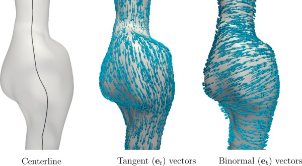
Unit vector field ${\mathbf{e}}_t$ is defined as the unit tangent vector that is most aligned with the centerline direction. The binormal vector ${\mathbf{e}}_b$ is computed as the cross product of this unit tangent vector and the unit normal vector.

$$\mathit{\tau }={\tau }_t{\mathbf{e}}_t+{\tau }_b{\mathbf{e}}_b$$ (3)

where ${\tau }_t=\mathit{\tau }·{\mathbf{e}}_t$ and ${\tau }_b=\mathit{\tau }·{\mathbf{e}}_b$ are the components of the WSS vector in tangent and binormal directions, respectively. In this paper, the WSS angle, θ, is defined as the angle between the WSS vector and the tangent direction

$$\theta =\arccos \frac{\mathit{\tau }·{\mathbf{e}}_t}{\Vert \mathit{\tau }\Vert }$$ (4)

2.2.1. WSS Parameters.

We begin by defining the standard WSS parameters used in literature. $\left|\right|\overline{\mathit{\tau }}\left|\right|$ is defined as the magnitude of the time average of WSS vector, where the averaging time is typically one cardiac cycle T assuming the flow is periodic

$$\left|\right|\overline{\mathit{\tau }}\left|\right|=\left|\right|\frac{1}{T}{\int }_0^T\mathit{\tau }\mathrm{d}t\left|\right|$$ (5)

The standard time average of WSS (magnitude) is defined as

$$\text{TAWSS}=\frac{1}{T}{\int }_0^T\Vert \mathit{\tau }\Vert \mathrm{d}t$$ (6)

The OSI is defined as

$$\text{OSI}=\frac{1}{2}\left(1-\frac{\left|\right|\overline{\mathit{\tau }}\left|\right|}{\text{TAWSS}}\right)$$ (7)

OSI becomes 0 for unidirectional WSS (steady direction) and 0.5 for WSS with no preferred time-averaged direction ($\left|\right|\overline{\mathit{\tau }}\left|\right|=0$). The values in between are not easily interpreted. We propose an additional measure to quantify WSS direction changes. ${\Delta }_{90}$ is defined as the number of instances that WSS angle θ changes more than 90 deg (or any desired threshold could be used), which can be computed as follows:

$t_0=0$, ${\Delta }_{90}=0$

for t = 0 to T do

if $\underset{t_0<t\prime <t}{\text{max}}|\theta (t)-\theta (t\prime )|>\pi /2$ then

${\Delta }_{90}\leftarrow {\Delta }_{90}+1$

$t_0\leftarrow t$

end if

end for

This measure inspects consecutive time steps to check when the WSS vector turns 90 deg, and then resets the reference direction for capturing the next 90 deg turn. Similar to Ref. [23], we define $\overline{|{\tau }_t|}$, and $\overline{|{\tau }_b|}$ as the integrated amount of WSS in tangent and binormal directions, respectively,

$$\begin{array}{cc}\overline{\left|{\tau }_t\right|}& =\frac{1}{T}{\int }_0^T\left|{\tau }_t\right|\mathrm{d}t\\ \overline{\left|{\tau }_b\right|}& =\frac{1}{T}{\int }_0^T\left|{\tau }_b\right|\mathrm{d}t\end{array}$$ (8)

These measures can quantify the persistent alignment of WSS to the centerline, or perpendicular to centerline, direction, respectively. WSS vector fields can be scaled to obtain a first-order approximation of near wall velocity vectors [25]. If sign is taken into account in above equations, then one can distinguish between persistent regions of forward and backward near wall flow, as well as clockwise and counterclockwise near-wall flow, providing some insight on near-wall transport. Specifically, backward WSS ($\overline{|{\tau }_{t^{-}}|}$) could be defined as the amount of near-wall backflow

$$\{\begin{array}{l}\overline{\left|{\tau }_{t^{-}}\right|}=\frac{1}{T}{\int }_0^T\left|H\left(t\right){\tau }_t\right|\mathrm{d}t\\ H(t)=\{\begin{array}{c}1\text{if}{\tau }_t<0\\ 0\text{if}{\tau }_t\ge 0\end{array}\end{array}$$ (9)

This measure could be used in quantification of recirculating flow, which has been shown to promote thrombotic and atherosclerosis expressions [37]. Table 1 lists various forms of spatial and temporal gradients that could be defined. The WSS angle and magnitude provide scalar fields that could be used to compute spatial/temporal gradients. The spatial/temporal gradient of the WSS vector can also be computed, which inherently incorporates both direction and magnitude changes. See the Appendix for details on angle gradient and vector gradient computations. A relative measure of WSS gradient can be defined by dividing the vector gradient by the WSS magnitude. All of the measures defined in Table 1 are integrated and divided in time similar to previous parameters.

Table 1.

Scalar measures quantifying spatial and temporal changes of WSS derived from WSS angle, magnitude, and vector. Relative measures are defined by dividing the variation by WSS magnitude. All of the measures would be averaged temporally. Prime denotes temporal gradient ($\prime =d/dt$). For $\Vert \nabla \mathit{\tau }\Vert$ the induced L₂ (spectral) norm was used.

	Space	Time
Angle	$\Vert \nabla \theta \Vert$	$\theta \prime$
Magnitude	$\Vert \nabla \Vert \mathit{\tau }\Vert \Vert$	$\Vert \mathit{\tau }\Vert \prime$
Vector	$\Vert \nabla \mathit{\tau }\Vert$	$\Vert \mathit{\tau }\prime \Vert$
Relative	$\frac{\Vert \nabla \mathit{\tau }\Vert }{\Vert \mathit{\tau }\Vert }$	$\frac{\Vert \mathit{\tau }\prime \Vert }{\Vert \mathit{\tau }\Vert }$

As will be shown in Sec. 3, the spatial (temporal) WSS vector gradient has very high positive correlation with spatial (temporal) WSS magnitude gradient. This motivated the definition of new measures that can incorporate magnitude and angle changes more equitably. We define a mix spatial gradient as a linear weighting of WSS angle and magnitude gradients, such that the new measure is equally correlated with angle and magnitude gradients as follows:

$$\begin{array}{cc}{\nabla }_{\text{mix}}\mathit{\tau }& =w_s\frac{\Vert \nabla \theta \Vert }{\text{mean}\left(\Vert \nabla \theta \Vert \right)}+\left(1-w_s\right)\frac{\Vert \nabla \Vert \mathit{\tau }\Vert \Vert }{\text{mean}\left(\Vert \nabla \Vert \mathit{\tau }\Vert \Vert \right)}\\ w_s:& \text{corr}\left({\nabla }_{\text{mix}}\mathit{\tau },\Vert \nabla \theta \Vert \right)=\text{corr}\left({\nabla }_{\text{mix}}\mathit{\tau },\Vert \nabla \Vert \mathit{\tau }\Vert \Vert \right)\end{array}$$ (10)

where the mean operator computes the spatial average of the parameter in the region of interest. The normalization by the mean provides a dimensionless parameter with mean value equal to one. The weighting coefficient w_s is chosen to provide equal correlation coefficients. A similar approach could be taken for WSS temporal gradient to define a mix temporal gradient

$$\begin{array}{cc}\mathit{\tau }{\prime }_{\text{mix}}& =w_t\frac{\theta \prime }{\text{mean}\left(\theta \prime \right)}+\left(1-w_t\right)\frac{\Vert \mathit{\tau }\Vert \prime }{\text{mean}\left(\Vert \mathit{\tau }\Vert \prime \right)}\\ w_t:& \text{corr}\left(\mathit{\tau }{\prime }_{\text{mix}},\theta \prime \right)=\text{corr}\left(\mathit{\tau }{\prime }_{\text{mix}},\Vert \mathit{\tau }\Vert \prime \right)\end{array}$$ (11)

where the weighting coefficient w_t provides equal correlation between the new measure and magnitude/angle temporal gradients. The spatial and temporal mix gradients could be combined to define a new measure ${\mathit{\tau }}_{\text{mix}}$ that incorporates spatial and temporal changes of magnitude and angle of WSS as follows:

$$\begin{array}{cc}{\mathit{\tau }}_{\text{mix}}& =w_{\mathit{s}\mathit{t}}{\nabla }_{\text{mix}}\mathit{\tau }+(1-w_{\mathit{s}\mathit{t}})\mathit{\tau }{\prime }_{\text{mix}}\\ w_{\mathit{s}\mathit{t}}:& \text{corr}({\mathit{\tau }}_{\text{mix}},{\nabla }_{\text{mix}}\mathit{\tau })=\text{corr}({\mathit{\tau }}_{\text{mix}},\mathit{\tau }{\prime }_{\text{mix}})\end{array}$$ (12)

where the weighting coefficient w_st results equal correlation of ${\mathit{\tau }}_{\text{mix}}$ with spatial and temporal mix gradients.

3. Results

The computational models used in this study are shown in Fig. 2. WSS correlations were performed in the shaded aneurysmal regions. Figure 3 shows some of the complex instantaneous vectorial WSS patterns observed in the AAA models.

Fig. 2.

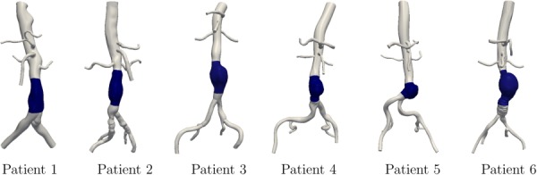
Patient-specific models used in this study. The shaded region shows the aneurysmal region, where the WSS correlations were performed.

Fig. 3.

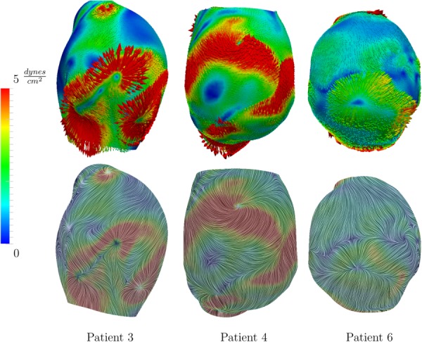
Instantaneous complex WSS vectors, and the corresponding WSS streamlines for three patients. To improve visualization, the WSS vectors are scaled differently in each patient; however the same color mapping was used among all cases.

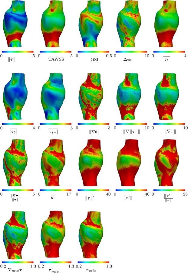
Figures 4 and 5 show all the defined WSS parameters of a representative case for anterior and posterior views, respectively. A pointwise correlation study was performed among all the WSS parameters for each anatomic model, using the Pearson correlation coefficient. These coefficients were computed from pointwise correlation of all the surface points for each patient separately, resulting in six coefficients. The mean Pearson correlation coefficient resulting from all the patients is listed in Table 2, with the statistically significant correlations among the six patients indicated. A one-sample t-test analysis was performed to compute the p-values based on the Pearson correlation coefficients obtained for each patient; therefore, the correlations that are not marked significant had notable interpatient variability.

Fig. 4.

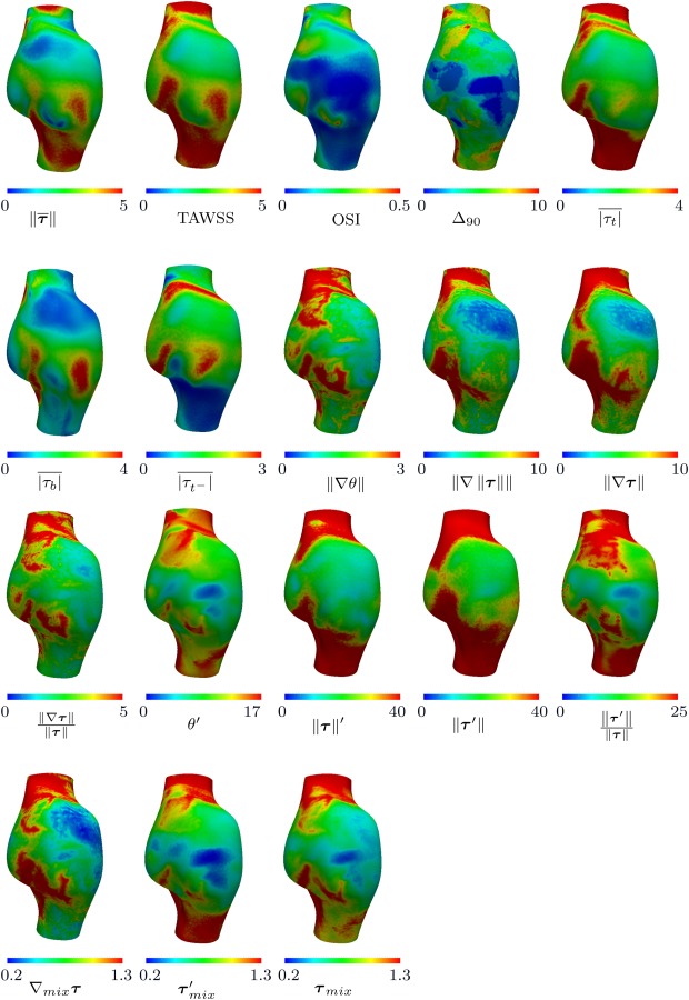
WSS parameters for a representative case (patient 3). The anterior view is shown in this figure. All units are based on $\text{dynes}/{\text{cm}}^2$ for WSS magnitude, radians for WSS angle, cm for spatial gradients, and seconds for time. OSI, ${\Delta }_{90}$ and mix parameters are dimensionless.

Fig. 5.

WSS parameters for a representative case (patient 3). The posterior view is shown in this figure. All units are based on $\text{dynes}/{\text{cm}}^2$ for WSS magnitude, rad for WSS angle, cm for spatial gradients, and seconds for time. OSI, ${\Delta }_{90}$ and mix parameters are dimensionless.

Table 2.

Pearson correlation coefficients among all the WSS parameters studied. Significant correlations (p  <  0.05) are shown in bold. Very significant correlations are marked with ** (p  <  0.01). Total of 13592 ± 3956 surface points were analyzed for each of the six patients.

	TAWSS	OSI	${\Delta }_{90}$	$\overline{|{\tau }_t|}$	$\overline{|{\tau }_b|}$	$\overline{|{\tau }_{t^{-}}|}$	$\Vert \nabla \theta \Vert$	$\Vert \nabla \Vert \mathit{\tau }\Vert \Vert$	$\Vert \nabla \mathit{\tau }\Vert$	$\frac{\Vert \nabla \mathit{\tau }\Vert }{\Vert \mathit{\tau }\Vert }$	$\theta \prime$	$\Vert \mathit{\tau }\Vert \prime$	$\Vert \mathit{\tau }\prime \Vert$	$\frac{\Vert \mathit{\tau }\prime \Vert }{\Vert \mathit{\tau }\Vert }$	${\nabla }_{\text{mix}}\mathit{\tau }$	$\mathit{\tau }{\prime }_{\text{mix}}$	${\mathit{\tau }}_{\text{mix}}$
$\left|\right|\overline{\mathit{\tau }}\left|\right|$	0.85**	−0.70**	−0.02	0.82**	0.49**	0.05	0.00	0.54**	0.51**	0.02	−0.01	0.64**	0.61**	0.05	0.32**	0.38**	0.39**
TAWSS		−0.35**	0.09	0.96**	0.59**	0.22	0.10	0.67**	0.67**	0.08	0.09	0.85**	0.85**	0.11	0.46**	0.56**	0.57**
OSI			0.22	−0.29**	−0.33	0.06	0.14	−0.18**	−0.15	0.08	0.19	−0.11	−0.09	0.13	−0.02	0.05	0.01
${\Delta }_{90}$				0.13	−0.10	−0.13	0.55**	0.19**	0.23**	0.42**	0.92**	0.36**	0.39**	0.52**	0.44**	0.77**	0.68**
$\overline{|{\tau }_t|}$					0.36**	0.21	0.11	0.65**	0.63**	0.09	0.12	0.86**	0.82**	0.16	0.45**	0.59**	0.58**
$\overline{|{\tau }_b|}$						0.18	0.02	0.39**	0.43**	−0.01	−0.07	0.37**	0.48**	−0.10	0.24**	0.18	0.24
$\overline{|{\tau }_{t^{-}}|}$							−0.04	0.14	0.15	−0.03	−0.19	0.12	0.13	−0.06	0.06	−0.05	0.01
$\Vert \nabla \theta \Vert$								0.41**	0.49**	0.75**	0.58**	0.30**	0.32**	0.38**	0.84**	0.52**	0.76**
$\Vert \nabla \Vert \mathit{\tau }\Vert \Vert$									0.98**	0.43**	0.20**	0.64**	0.65**	0.15	0.84**	0.50**	0.75**
$\Vert \nabla \mathit{\tau }\Vert$										0.48**	0.25**	0.65**	0.68**	0.16	0.87**	0.54**	0.79**
$\frac{\Vert \nabla \mathit{\tau }\Vert }{\Vert \mathit{\tau }\Vert }$											0.44**	0.22**	0.22**	0.52**	0.70**	0.40**	0.62**
$\theta \prime$												0.39	0.43	0.54**	0.46**	0.83**	0.73**
$\Vert \mathit{\tau }\Vert \prime$													0.97**	0.30**	0.56**	0.83**	0.77**
$\Vert \mathit{\tau }\prime \Vert$														0.28**	0.58**	0.84**	0.78**
$\frac{\Vert \mathit{\tau }\prime \Vert }{\Vert \mathit{\tau }\Vert }$															0.31**	0.51	0.45
${\nabla }_{\text{mix}}\mathit{\tau }$																0.61**	0.89**
$\mathit{\tau }{\prime }_{\text{mix}}$																	0.90**

Several observations are made from this table:

• (1)TAWSS is highly correlated with $\left|\right|\overline{\mathit{\tau }}\left|\right|$.
• (2)WSS magnitude spatial gradient and WSS vector spatial gradient are highly correlated with correlation coefficient close to one. Similar observation is made for WSS temporal gradients.
• (3)The high positive correlation of TAWSS with WSS magnitude/vector spatial and temporal gradient motivates the definition of relative WSS spatial gradient ($\Vert \nabla \mathit{\tau }\Vert /\Vert \mathit{\tau }\Vert$) and relative WSS temporal gradient ($\left|\right|\mathit{\tau }\prime \left|\right|/\Vert \mathit{\tau }\Vert$). These new measures are no longer correlated with TAWSS, and at the same time have relatively moderate correlation with WSS gradients.
• (4)Angle based measures (${\Delta }_{90},\hspace{0.17em}\nabla \theta ,\hspace{0.17em}\theta \prime$) are uncorrelated to TAWSS.
• (5)Comparison of $\overline{|{\tau }_t|}$ and $\overline{|{\tau }_b|}$ correlations shows that $\overline{|{\tau }_b|}$ is less correlated with spatial and temporal changes of WSS.
• (6)${\mathit{\tau }}_{\text{mix}}$ is moderately to strongly correlated to all the parameters with high statistical significance, except to OSI, $\overline{|{\tau }_b|}$ and $\overline{|{\tau }_{t^{-}}|}$.

The weighting coefficients used for the mix WSS parameters in Eqs. (10)–(12) were found to be $w_s=0.62\pm 0.04,\hspace{0.17em}{w}_t=0.63\pm 0.05,\hspace{0.17em}{w}_{\mathit{s}\mathit{t}}=0.40\pm 0.05$ for the present data.

Removing the absolute value from the definition of $\overline{|{\tau }_t|}$ in Eq. (8) enables one to distinguish between regions of dominant forward and backward near wall flow, as shown in Fig. 6. The positive regions in the figure represent dominant forward WSS vectors, whereas the negative regions indicate dominant backward WSS vectors. Similarly, removing the absolute values in the $\overline{|{\tau }_b|}$ definition of Eq. (8) enables the distinction between dominant clockwise and counterclockwise rotating near-wall flows, as shown in Fig. 7. The positive regions show dominant counterclockwise WSS vectors, whereas the negative regions show dominant clockwise WSS vectors. The ratio of $\overline{|{\tau }_b|}$ to TAWSS was found to be on average 0.38 ± 0.06 for each patient.

Fig. 6.

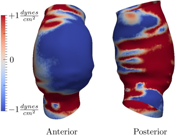
Sum of WSS vectors in the tangent direction (${\int }_0^T{\tau }_t\mathrm{d}t$) for a representative case (patient 4). Positive values show regions with dominant forward near wall flow. Negative values show regions with dominant backward near wall flow. The colorbar range does not represent peak values.

Fig. 7.

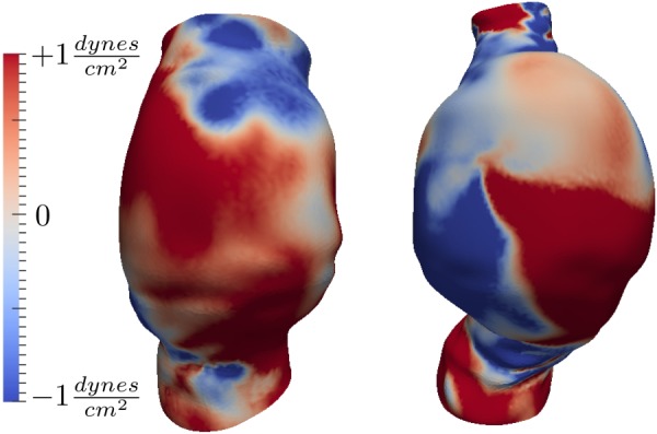
Sum of WSS vectors in the binormal direction (${\int }_0^T{\tau }_b\mathrm{d}t$) for two representative cases (patients 4 and 6). Anterior views are shown. Positive values show regions with dominant counterclockwise near wall rotating flow. Negative values show regions with dominant clockwise near wall rotating flow. The colorbar range does not represent peak values.

The effects of surface curvature on the WSS vector gradient appears to have been mostly overlooked in the literature. These effects were investigated in this study (see the Appendix for the formulation) and it was found that including the curvature terms into the gradient changed the correlation coefficients less than 0.01 for our data, which provides justification for prior works that have neglected this effect.

4. Discussion

WSS is a vectorial quantity, with often complicated spatial and temporal variation. These factors can confound both the quantification and interpretation of WSS in cardiovascular flows. While traditional TAWSS is treated as a scalar quantity, the vectorial nature of WSS and its gradients vastly increase the dimensionality of WSS data, and possibilities for how it can be quantified. Therefore, it is fruitful to consider how various quantifications correlate to reduce the possible parameters needed to effectively quantify or interpret hemodynamics data.

Various WSS parameters and their correlations in complex arterial flow have been investigated. Several WSS metrics were considered, and emphasis was placed on the temporal and spatial fluctuations of WSS angle, magnitude, and vector in space and time. The correlation results showed high positive correlation of vectorial spatial (temporal) gradient of WSS with its magnitude spatial (temporal) gradient. While fluctuations in WSS are affected by both changes in magnitude and direction (angle), the correlation results show there is a strong bias of WSS vectorial changes with magnitude changes. This motivated the definition of mix WSS spatial (temporal) gradient to incorporate spatial (temporal) changes of angle and magnitude into single measures. These measures were then combined to derive a mix WSS, ${\mathit{\tau }}_{\text{mix}}$, parameter, which demonstrated statistically significant positive correlation (moderate to strong) with all of the WSS parameters except OSI, $\overline{|{\tau }_b|}$ and $\overline{|{\tau }_{t^{-}}|}$.

Relatively high positive correlation between TAWSS and WSS spatial/temporal gradient was observed, consistent with previous findings in carotid arteries [24]. This should not be surprising, since small relative changes of WSS in a high shear region can lead to a higher spatial/temporal gradient than large relative changes of WSS in a low shear region. Therefore, high shear regions are biased to produce higher gradients. This motivated the definition of relative gradients. These relative measures were uncorrelated to TAWSS, while they had relatively moderate correlation with WSS gradients. These differences should be contextualized from the perspective of the cells in contact with blood flow. Large relative spatial fluctuations among WSS vectors with small magnitude will likely lead to small measured gradients. However, these small gradients may be as significant to ECs as high gradients resulting from relatively minor changes among large magnitude WSS. The same could be said for temporal gradients. For example, high gradients in WSS are observed in regions of flow dividers that are usually atherosclerosis free, while the likely smaller in magnitude WSS gradients in regions of recirculation promote atherosclerosis [38]. Hence, although relative gradient measures should not replace absolute gradient measures, they should serve as additional measures to guide the interpretation of WSS gradients.

In this study, we observed a very weak positive correlation between TAWSS and WSS angle gradients. Lee et al. [24] have reported a relatively weak negative correlation between these measures in carotid arteries. Moreover, the correlations between WSS angle gradient and other measures considered in that study were also different than observed herein. The discrepancy may be due to the modified definition of WSS angle gradient in this study, or the different flow environments. Otherwise, the correlations in common between these two studies were in relative agreement.

In this paper, we used a wall tangent direction aligned with the nominal direction of flow as the reference direction for quantifying directional variations in WSS. This approach is particularly suitable if one is interested in WSS as a measure characterizing near wall transport. The WSS vectors are indicators of flow topology next to the wall. Their role in transport of biochemicals near the wall becomes particularly significant if transport of biochemicals from the wall is confined to a thin boundary layer next to the wall [39]. This happens in transport of biochemicals with high Schmidt number, which is typically the case in cardiovascular applications [40]. Most studies use the TAWSS direction in their characterizations, being motivated by the fact that the cells prefer to align to the time average direction of the WSS vector. However, in complex flows such as aneurysms the time average direction will yield a reference direction that is dependent on the complexities involved in flow behavior. Therefore, measures based on the TAWSS direction confound interpretation of WSS variations in complex flows. Moreover, the time average direction can become prone to numerical errors in regions of low WSS, typically seen in aneurysms.

It is noteworthy that the aneurysm formation indicator measure [19,41] defined as $\text{AFI}=\mathit{\tau }·\overline{\mathit{\tau }}/\Vert \mathit{\tau }\Vert \left|\right|\overline{\mathit{\tau }}\left|\right|$ is similar to $\overline{|{\tau }_t|}$ used in this study, where the time average direction $\overline{\mathit{\tau }}$ is replaced by ${\mathbf{e}}_t$ (Eq. (2)) and magnitude is taken into account. The transWSS measure [21,22] defined as the average magnitude of WSS perpendicular to the $\overline{\mathit{\tau }}$ direction is similar to $\overline{|{\tau }_b|}$, where the time average direction is replaced by ${\mathbf{e}}_t$. Recently, Morbiducci et al. [23] used a similar approach to what is used in this study to define axial and secondary WSS similar to $\overline{|{\tau }_t|}$ and $\overline{|{\tau }_b|}$, respectively. In their study, axial and secondary WSS were directly projected to the centerline and perpendicular to centerline directions, producing WSS components that do not lie in the local tangent plane, whereas the approach herein used projections that lie in the local tangent plane.

The correlation results demonstrated a lower correlation of $\overline{|{\tau }_b|}$ with spatial/temporal changes of WSS angle and magnitude, compared to $\overline{|{\tau }_t|}$. The increase in $\overline{|{\tau }_b|}$ can be due to the helical nature of flow [42], suggesting that this type of flow can reduce the spatial and temporal changes in WSS. This finding is consistent with prior studies in carotid arteries where helical flow has been shown to suppress disturbed flow, and contribute to uniformity in WSS [43]. Helical flow can reduce the accumulation of specific atherogenic chemicals on the vessel wall, and prevent platelet adhesion to the vessel wall, therefore protecting against atherosclerosis and thrombosis, respectively [44]. These protective mechanisms are due to the modification of near wall transport topology, which is manifested in the WSS vector field.

In this study, we only used one cardiac cycle of WSS data for our calculations. It has been shown that in transitional flows such as AAAs, time-averaged WSS measures might need several cardiac cycles to converge [45]. However, the purpose of our study was to compute correlations across parameters, therefore this issue is not expected to affect our results significantly. Nevertheless, care must be taken when correlating time-averaged WSS parameters to different aspects of AAA disease.

The capability of ECs to respond to the local flow patterns [46], along with the realization that the WSS vector field is important in determining near wall transport, brings the need for renewed perspectives in WSS characterizations. Indeed, the prevailing theory of association of low and oscillatory WSS with atherosclerosis has been questioned [47], and conflicting results regarding the common belief about low WSS and high OSI have been reported [22,36]. These findings encourage further attention in revisiting the traditional approaches used in WSS characterizations and their correlation with disease.

Appendix

A.1. Angle Gradients

When computing the difference between two angles, one must take care to account for the discontinuity in quantifying angle (e.g., passing between $-\pi$ and π or 0 and $2\pi$). For example, in Fig. 8(a) if ${\alpha }_1\approx \mathrm{ϵ}$ and $2\pi -{\alpha }_2\approx \mathrm{ϵ}$ are small angles, the computed change in angle will be $\approx 2\pi$, while the actual change is very small ($2\mathrm{ϵ}$). To overcome this issue, another reference direction $-{\mathbf{e}}_t$ is introduced and a new angle ${\theta }_2$ is measured with respect to this direction in the clockwise direction, as shown in Fig. 8(b). The change in WSS angle is equal to the minimum of the two angle changes

Fig. 8.

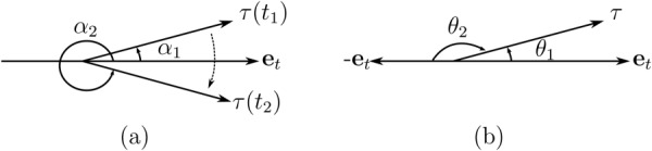
(a) Changes in WSS angle can be computed wrong in regions near the transition of the coordinate (between 0 and 2π using the convention shown). (b) Quantification of changes in WSS angle can be achieved by computation of WSS angle with respect to two reference directions and taking the minimum of the two differences.

$$\Delta \theta =\text{min}\left\{\right|{\theta }_1(b)-{\theta }_1(a)|,|{\theta }_2(b)-{\theta }_2(a)\left|\right\}$$ (A1)

where a and b could be two points in space or time, and Δ can be the spatial/temporal gradients or any other measure that quantifies changes in angle.

A.2. WSS Vector Gradient

In the Cartesian coordinates WSS can be written as $\mathit{\tau }={\tau }_x\widehat{\mathbf{i}}+{\tau }_y\widehat{\mathbf{j}}+{\tau }_z\widehat{\mathbf{k}}$. The WSS gradient becomes

$${\nabla }_{\mathit{x}\mathit{y}\mathit{z}}\mathit{\tau }=\left[\begin{array}{ccc}\frac{\partial {\tau }_x}{\partial x}& \frac{\partial {\tau }_x}{\partial y}& \frac{\partial {\tau }_x}{\partial z}\\ \frac{\partial {\tau }_y}{\partial x}& \frac{\partial {\tau }_y}{\partial y}& \frac{\partial {\tau }_y}{\partial z}\\ \frac{\partial {\tau }_z}{\partial x}& \frac{\partial {\tau }_z}{\partial y}& \frac{\partial {\tau }_z}{\partial z}\end{array}\right]$$ (A2)

It is necessary to transform the gradient to the local intrinsic frame (${\mathbf{e}}_t,{\mathbf{e}}_b,{\mathbf{e}}_n$), and remove the normal contributions to the gradient, this will result in

$$\nabla \mathit{\tau }=\left[\begin{array}{cc}{\mathbf{e}}_t^{\mathrm{⊺}}·[\begin{array}{c}{\nabla }_{\mathit{x}\mathit{y}\mathit{z}}\mathit{\tau }\end{array}]·{\mathbf{e}}_t& {\mathbf{e}}_t^{\mathrm{⊺}}·[\begin{array}{c}{\nabla }_{\mathit{x}\mathit{y}\mathit{z}}\mathit{\tau }\end{array}]·{\mathbf{e}}_b\\ {\mathbf{e}}_b^{\mathrm{⊺}}·[\begin{array}{c}{\nabla }_{\mathit{x}\mathit{y}\mathit{z}}\mathit{\tau }\end{array}]·{\mathbf{e}}_t& {\mathbf{e}}_b^{\mathrm{⊺}}·[\begin{array}{c}{\nabla }_{\mathit{x}\mathit{y}\mathit{z}}\mathit{\tau }\end{array}]·{\mathbf{e}}_b\end{array}\right]$$ (A3)

The induced L₂ norm of this matrix has been used in Sec.

The fact that the gradient is acting on a surface manifold, requires incorporation of curvature effects into the gradient. This can be done by computing the Ricci rotation coefficients [48]

$${\gamma }_{\mathit{a}\mathit{b}\mathit{c}}={\widehat{\mathbf{e}}}_a^{\mathrm{⊺}}·[\begin{array}{c}{\nabla }_{\mathit{x}\mathit{y}\mathit{z}}{\widehat{\mathbf{e}}}_b\end{array}]·{\widehat{\mathbf{e}}}_c$$ (A4)

where (${\widehat{\mathbf{e}}}_1,{\widehat{\mathbf{e}}}_2,{\widehat{\mathbf{e}}}_3$) = (${\mathbf{e}}_t,{\mathbf{e}}_b,{\mathbf{e}}_n$) are the basis used. The final form of WSS gradient can be written as

$${\nabla }_S\mathit{\tau }=\nabla \mathit{\tau }-\left[\begin{array}{cc}{\gamma }_{111}{\tau }_t+{\gamma }_{211}{\tau }_b& {\gamma }_{112}{\tau }_t+{\gamma }_{212}{\tau }_b\\ {\gamma }_{121}{\tau }_t+{\gamma }_{221}{\tau }_b& {\gamma }_{122}{\tau }_t+{\gamma }_{222}{\tau }_b\end{array}\right]$$ (A5)

where τ_t and τ_b are the components of WSS vector in the ${\mathbf{e}}_t$ and ${\mathbf{e}}_b$ directions, respectively. Note that the normal component of WSS is zero by definition and does not appear in Eq. (A5).

References

- [1]. Barakat, A. I. , and Lieu, D. K. , 2003, “ Differential Responsiveness of Vascular Endothelial Cells to Different Types of Fluid Mechanical Shear Stress,” Cell Biochem. Biophys., 38(3), pp. 323–343. 10.1385/CBB:38:3:323 [DOI] [PubMed] [Google Scholar]
- [2]. Lu, D. , and Kassab, G. S. , 2011, “ Role of Shear Stress and Stretch in Vascular Mechanobiology,” J. R. Soc., Interface, 8(63), pp. 1379–1385. 10.1016/j.jbiomech.2009.09.012 [DOI] [PMC free article] [PubMed] [Google Scholar]
- [3]. Chiu, J. J. , and Chien, S. , 2011, “ Effects of Disturbed Flow on Vascular Endothelium: Pathophysiological Basis and Clinical Perspectives,” Physiol. Rev., 91(1), pp. 327–387. 10.1152/physrev.00047.2009 [DOI] [PMC free article] [PubMed] [Google Scholar]
- [4]. Archie, J. P., Jr. , Hyun, S. , Kleinstreuer, C. , Longest, P. W. , Truskey, G. A. , and Buchanan, J. R. , 2001, “ Hemodynamic Parameters and Early Intimal Thickening in Branching Blood Vessels,” Crit. Rev. Biomed. Eng., 29(1), pp. 1–64. 10.1615/CritRevBiomedEng.v29.i1.10 [DOI] [PubMed] [Google Scholar]
- [5]. Gallo, D. , Isu, G. , Massai, D. , Pennella, F. , Deriu, M. A. , Ponzini, R. , Bignardi, C. , Audenino, A. , Rizzo, G. , and Morbiducci, U. , 2014, “ A Survey of Quantitative Descriptors of Arterial Flows,” Visualization and Simulation of Complex Flows in Biomedical Engineering, Springer, Dordrecht, pp. 1–24. [Google Scholar]
- [6]. Ostrowski, M. A. , Huang, N. F. , Walker, T. W. , Verwijlen, T. , Poplawski, C. , Khoo, A. S. , Cooke, J. P. , Fuller, G. G. , and Dunn, A. R. , 2014, “ Microvascular Endothelial Cells Migrate Upstream and Align Against the Shear Stress Field Created by Impinging Flow,” Biophys. J., 106(2), pp. 366–374. 10.1016/j.bpj.2013.11.4502 [DOI] [PMC free article] [PubMed] [Google Scholar]
- [7]. Meng, H. , Tutino, V. M. , Xiang, J. , and Siddiqui, A. , 2013, “ High WSS or Low WSS? Complex Interactions of Hemodynamics With Intracranial Aneurysm Initiation, Growth, and Rupture: Toward a Unifying Hypothesis,” Am. J. Neuroradiol., 35(7), pp. 1254–1262. 10.3174/ajnr.A3558 [DOI] [PMC free article] [PubMed] [Google Scholar]
- [8]. Watton, P. N. , Selimovic, A. , Raberger, N. B. , Huang, P. , Holzapfel, G. A. , and Ventikos, Y. , 2011, “ Modelling Evolution and the Evolving Mechanical Environment of Saccular Cerebral Aneurysms,” Biomech. Model. Mechanobiol., 10(1), pp. 109–132. 10.1007/s10237-010-0221-y [DOI] [PubMed] [Google Scholar]
- [9]. Ku, D. N. , Giddens, D. P. , Zarins, C. K. , and Glagov, S. , 1985, “ Pulsatile Flow and Atherosclerosis in the Human Carotid Bifurcation. Positive Correlation Between Plaque Location and Low Oscillating Shear Stress,” Arterioscler., Thromb., Vasc. Biol., 5(3), pp. 293–302. 10.1161/01.ATV.5.3.293 [DOI] [PubMed] [Google Scholar]
- [10]. Knight, J. , Olgac, U. , Saur, S. C. , Poulikakos, D. , Marshall, W., Jr. , Cattin, P. C. , Alkadhi, H. , and Kurtcuoglu, V. , 2010, “ Choosing the Optimal Wall Shear Parameter for the Prediction of Plaque Location—A Patient-Specific Computational Study in Human Right Coronary Arteries,” Atherosclerosis, 211(2), pp. 445–450. 10.1016/j.atherosclerosis.2010.03.001 [DOI] [PubMed] [Google Scholar]
- [11]. Buchanan, J. R., Jr. , Kleinstreuer, C. , Truskey, G. A. , and Lei, M. , 1999, “ Relation Between Non-Uniform Hemodynamics and Sites of Altered Permeability and Lesion Growth at the Rabbit Aorto-Celiac Junction,” Atherosclerosis, 143(1), pp. 27–40. 10.1016/S0021-9150(98)00264-0 [DOI] [PubMed] [Google Scholar]
- [12]. Dolan, J. M. , Kolega, J. , and Meng, H. , 2013, “ High Wall Shear Stress and Spatial Gradients in Vascular Pathology: A Review,” Ann. Biomed. Eng., 41(7), pp. 1411–1427. 10.1007/s10439-012-0695-0 [DOI] [PMC free article] [PubMed] [Google Scholar]
- [13]. Buchanan, J. R. , Kleinstreuer, C. , Hyun, S. , and Truskey, G. A. , 2003, “ Hemodynamics Simulation and Identification of Susceptible Sites of Atherosclerotic Lesion Formation in a Model Abdominal Aorta,” J. Biomech., 36(8), pp. 1185–1196. 10.1016/S0021-9290(03)00088-5 [DOI] [PubMed] [Google Scholar]
- [14]. White, C. R. , Haidekker, M. , Bao, X. , and Frangos, J. A. , 2001, “ Temporal Gradients in Shear, But Not Spatial Gradients, Stimulate Endothelial Cell Proliferation,” Circulation, 103(20), pp. 2508–2513. 10.1161/01.CIR.103.20.2508 [DOI] [PubMed] [Google Scholar]
- [15]. Dolan, J. M. , Meng, H. , Singh, S. , Paluch, R. , and Kolega, J. , 2011, “ High Fluid Shear Stress and Spatial Shear Stress Gradients Affect Endothelial Proliferation, Survival, and Alignment,” Ann. Biomed. Eng., 39(6), pp. 1620–1631. 10.1007/s10439-011-0267-8 [DOI] [PMC free article] [PubMed] [Google Scholar]
- [16]. Van Wyk, S. , Wittberg, L. P. , and Fuchs, L. , 2014, “ Atherosclerotic Indicators for Blood-Like Fluids in 90-degree Arterial-Like Bifurcations,” Comput. Biol. Med., 50, pp. 56–69. 10.1016/j.compbiomed.2014.03.006 [DOI] [PubMed] [Google Scholar]
- [17]. Browne, L. D. , O'Callaghan, S. , Hoey, D. A. , Griffin, P. , McGloughlin, T. M. , and Walsh, M. T. , 2014, “ Correlation of Hemodynamic Parameters to Endothelial Cell Proliferation in an End to Side Anastomosis,” Cardiovasc. Eng. Technol., 5(1), pp. 110–118. 10.1007/s13239-013-0172-4 [DOI] [Google Scholar]
- [18]. Shimogonya, Y. , Ishikawa, T. , Imai, Y. , Matsuki, N. , and Yamaguchi, T. , 2009, “ Can Temporal Fluctuation in Spatial Wall Shear Stress Gradient Initiate a Cerebral Aneurysm? A Proposed Novel Hemodynamic Index, the Gradient Oscillatory Number (GON),” J. Biomech., 42(4), pp. 550–554. 10.1016/j.jbiomech.2008.10.006 [DOI] [PubMed] [Google Scholar]
- [19]. Chen, H. , Selimovic, A. , Thompson, H. , Chiarini, A. , Penrose, J. , Ventikos, Y. , and Watton, P. N. , 2013, “ Investigating the Influence of Haemodynamic Stimuli on Intracranial Aneurysm Inception,” Ann. Biomed. Eng., 41(7), pp. 1492–1504. 10.1007/s10439-013-0794-6 [DOI] [PubMed] [Google Scholar]
- [20]. Chakraborty, A. , Chakraborty, S. , Jala, V . R. , Haribabu, B. , Sharp, M. K. , and Berson, R. E. , 2012, “ Effects of Biaxial Oscillatory Shear Stress on Endothelial Cell Proliferation and Morphology,” Biotechnol. Bioeng., 109(3), pp. 695–707. 10.1002/bit.24352 [DOI] [PubMed] [Google Scholar]
- [21]. Peiffer, V. , Sherwin, S. J. , and Weinberg, P. D. , 2013, “ Computation in the Rabbit Aorta of a New Metric—The Transverse Wall Shear Stress—To Quantify the Multidirectional Character of Disturbed Blood Flow,” J. Biomech., 46(15), pp. 2651–2658. 10.1016/j.jbiomech.2013.08.003 [DOI] [PMC free article] [PubMed] [Google Scholar]
- [22]. Mohamied, Y. , Rowland, E. M. , Bailey, E. L. , Sherwin, S. J. , Schwartz, M. A. , and Weinberg, P. D. , 2014, “ Change of Direction in the Biomechanics of Atherosclerosis,” Ann. Biomed. Eng., 43(1), pp. 16–25. 10.1007/s10439-014-1095-4 [DOI] [PMC free article] [PubMed] [Google Scholar]
- [23]. Morbiducci, U. , Gallo, D. , Cristofanelli, S. , Ponzini, R. , Deriu, M. A. , Rizzo, G. , and Steinman, D. A. , 2015, “ A Rational Approach to Defining Principal Axes of Multidirectional Wall Shear Stress in Realistic Vascular Geometries, With Application to the Study of the Influence of Helical Flow on Wall Shear Stress Directionality in Aorta,” J. Biomech., 48(6), pp. 899–906. 10.1016/j.jbiomech.2015.02.027 [DOI] [PubMed] [Google Scholar]
- [24]. Lee, S. W. , Antiga, L. , and Steinman, D. A. , 2009, “ Correlations Among Indicators of Disturbed Flow at the Normal Carotid Bifurcation,” ASME J. Biomech. Eng., 131(6), p. 061013. 10.1115/1.3127252 [DOI] [PubMed] [Google Scholar]
- [25]. Gambaruto, A. M. , Doorly, D. J. , and Yamaguchi, T. , 2010, “ Wall Shear Stress and Near-Wall Convective Transport: Comparisons With Vascular Remodelling in a Peripheral Graft Anastomosis,” J. Comput. Phys., 229(14), pp. 5339–5356. 10.1016/j.jcp.2010.03.029 [DOI] [Google Scholar]
- [26]. Gambaruto, A. M. , and João, A. J. , 2012, “ Flow Structures in Cerebral Aneurysms,” Comput. Fluids, 65, pp. 56–65. 10.1016/j.compfluid.2012.02.020 [DOI] [Google Scholar]
- [27]. El Hassan, M. , Assoum, H. H. , Martinuzzi, R. , Sobolik, V. , Abed-Meraim, K. , and Sakout, A. , 2013, “ Experimental Investigation of the Wall Shear Stress in a Circular Impinging Jet,” Phys. Fluids, 25(7), p. 077101. 10.1063/1.4811172 [DOI] [Google Scholar]
- [28]. Hansen, K. , and Shadden, S. , 2015, “ A Reduced-Dimensional Model for Near-Wall Transport in Cardiovascular Flows,” Biomech. Model. Mechanobiol., epub. 10.1007/s10237-015-0719-4 [DOI] [PMC free article] [PubMed] [Google Scholar]
- [29]. Conway, D. E. , and Schwartz, M. A. , 2013, “ Flow-Dependent Cellular Mechanotransduction in Atherosclerosis,” J. Cell Sci., 126(22), pp. 5101–5109. 10.1242/jcs.138313 [DOI] [PMC free article] [PubMed] [Google Scholar]
- [30]. John, K. , and Barakat, A. I. , 2001, “ Modulation of ATP/ADP Concentration at the Endothelial Surface by Shear Stress: Effect of Flow-Induced ATP Release,” Ann. Biomed. Eng., 29(9), pp. 740–751. 10.1114/1.1397792 [DOI] [PubMed] [Google Scholar]
- [31]. Arzani, A. , and Shadden, S. C. , 2012, “ Characterization of the Transport Topology in Patient-Specific Abdominal Aortic Aneurysm Models,” Phys. Fluids, 24(8), p. 081901. 10.1063/1.4744984 [DOI] [PMC free article] [PubMed] [Google Scholar]
- [32]. Arzani, A. , Les, A. S. , Dalman, R. L. , and Shadden, S. C. , 2014, “ Effect of Exercise on Patient Specific Abdominal Aortic Aneurysm Flow Topology and Mixing,” Int. J. Numer. Methods Biomed. Eng., 30(2), pp. 280–295. 10.1002/cnm.2601 [DOI] [PMC free article] [PubMed] [Google Scholar]
- [33]. Taylor, C. A. , Hughes, T. J. R. , and Zarins, C. K. , 1998, “ Finite Element Modeling of Blood Flow in Arteries,” Comput. Methods Appl. Mech. Eng., 158(1), pp. 155–196. 10.1016/S0045-7825(98)80008-X [DOI] [Google Scholar]
- [34]. Jansen, K. E. , Whiting, C. H. , and Hulbert, G. M. , 2000, “ A Generalized-Alpha Method for Integrating the Filtered Navier-Stokes Equations With a Stabilized Finite Element Method,” Comput. Methods Appl. Mech. Eng., 190(3–4), pp. 305–319. 10.1016/S0045-7825(00)00203-6 [DOI] [Google Scholar]
- [35]. Les, A. S. , Shadden, S. C. , Figueroa, C. A. , Park, J. M. , Tedesco, M. M. , Herfkens, R. J. , Dalman, R. L. , and Taylor, C. A. , 2010, “ Quantification of Hemodynamics in Abdominal Aortic Aneurysms During Rest and Exercise Using Magnetic Resonance Imaging and Computational Fluid Dynamics,” Ann. Biomed. Eng., 38(4), pp. 1288–1313. 10.1007/s10439-010-9949-x [DOI] [PMC free article] [PubMed] [Google Scholar]
- [36]. Arzani, A. , Suh, G. Y. , Dalman, R. L. , and Shadden, S. C. , 2014, “ A Longitudinal Comparison of Hemodynamics and Intraluminal Thrombus Deposition in Abdominal Aortic Aneurysms,” Am. J. Physiol.: Heart Circ. Physiol., 307, pp. H1786–H1795. 10.1152/ajpheart.00461.2014 [DOI] [PMC free article] [PubMed] [Google Scholar]
- [37]. Martorell, J. , Santomá, P. , Kolandaivelu, K. , Kolachalama, V . B. , Melgar-Lesmes, P. , Molins, J. J. , Garcia, L. , Edelman, E. R. , and Balcells, M. , 2014, “ Extent of Flow Recirculation Governs Expression of Atherosclerotic and Thrombotic Biomarkers in Arterial Bifurcations,” Cardiovasc. Res., 103(1), pp. 37–46. 10.1093/cvr/cvu124 [DOI] [PMC free article] [PubMed] [Google Scholar]
- [38]. Barbee, K. A. , 2002, “ Role of Subcellular Shear–Stress Distributions in Endothelial Cell Mechanotransduction,” Ann. Biomed. Eng., 30(4), pp. 472–482. 10.1114/1.1467678 [DOI] [PubMed] [Google Scholar]
- [39]. Kuharsky, A. L. , and Fogelson, A. L. , 2001, “ Surface-Mediated Control of Blood Coagulation: The Role of Binding Site Densities and Platelet Deposition,” Biophys. J., 80(3), pp. 1050–1074. 10.1016/S0006-3495(01)76085-7 [DOI] [PMC free article] [PubMed] [Google Scholar]
- [40]. Ethier, C. R. , 2002, “ Computational Modeling of Mass Transfer and Links to Atherosclerosis,” Ann. Biomed. Eng., 30(4), pp. 461–471. 10.1114/1.1468890 [DOI] [PubMed] [Google Scholar]
- [41]. Mantha, A. , Karmonik, C. , Benndorf, G. , Strother, C. , and Metcalfe, R. , 2006, “ Hemodynamics in a Cerebral Artery Before and After the Formation of an Aneurysm,” Am. J. Neuroradiol., 27(5), pp. 1113–1118. [PMC free article] [PubMed] [Google Scholar]
- [42]. Stalder, A. F. , Russe, M. F. , Frydrychowicz, A. , Bock, J. , Hennig, J. , and Markl, M. , 2008, “ Quantitative 2D and 3D Phase Contrast MRI: Optimized Analysis of Blood Flow and Vessel Wall Parameters,” Magn. Reson. Med., 60(5), pp. 1218–1231. 10.1002/mrm.21778 [DOI] [PubMed] [Google Scholar]
- [43]. Gallo, D. , Steinman, D. A. , Bijari, P. B. , and Morbiducci, U. , 2012, “ Helical Flow in Carotid Bifurcation as Surrogate Marker of Exposure to Disturbed Shear,” J. Biomech., 45(14), pp. 2398–2404. 10.1016/j.jbiomech.2012.07.007 [DOI] [PubMed] [Google Scholar]
- [44]. Liu, X. , Sun, A. , Fan, Y. , and Deng, X. , 2015, “ Physiological Significance of Helical Flow in the Arterial System and Its Potential Clinical Applications,” Ann. Biomed. Eng., 43(1), pp. 3–15. 10.1007/s10439-014-1097-2 [DOI] [PubMed] [Google Scholar]
- [45]. Poelma, C. , Watton, P. N. , and Ventikos, Y. , 2015, “ Transitional Flow in Aneurysms and the Computation of Haemodynamic Parameters,” J. R. Soc., Interface, 12(105), p. 20141394. 10.1016/S0140-6736(03)13860-3 [DOI] [PMC free article] [PubMed] [Google Scholar]
- [46]. Kataoka, N. , Ujita, S. , and Sato, M. , 1998, “ Effect of Flow Direction on the Morphological Responses of Cultured Bovine Aortic Endothelial Cells,” Med. Biol. Eng. Comput., 36(1), pp. 122–128. 10.1007/BF02522869 [DOI] [PubMed] [Google Scholar]
- [47]. Peiffer, V. , Sherwin, S. J. , and Weinberg, P. D. , 2013, “ Does Low and Oscillatory Wall Shear Stress Correlate Spatially With Early Atherosclerosis? A Systematic Review,” Cardiovasc. Res., 99, pp. 242–250. 10.1093/cvr/cvt044 [DOI] [PMC free article] [PubMed] [Google Scholar]
- [48]. Cherubini, C. , Filippi, S. , Gizzi, A. , and Nestola, M. G. C. , 2015, “ On the Wall Shear Stress Gradient in Fluid Dynamics,” Commun. Comput. Phys., 17(3), pp. 808–821. 10.4208/cicp.030714.101014a [DOI] [Google Scholar]