Anatomy and function of an excitatory network in the visual cortex

Abstract

Circuits in the cerebral cortex consist of thousands of neurons connected by millions of synapses. A precise understanding of these local networks requires relating circuit activity with the underlying network structure. For pyramidal cells in superficial mouse visual cortex (V1), a consensus is emerging that neurons with similar visual response properties excite each other^1–5, but the anatomical basis of this recurrent synaptic network is unknown. We combined physiological imaging and large-scale electron microscopy (EM) to study an excitatory network in V1. We found that layer 2/3 neurons organized into subnetworks defined by anatomical connectivity, with more connections within than between groups. More specifically, we found that pyramidal neurons with similar orientation selectivity preferentially formed synapses with each other, despite the fact that axons and dendrites of all orientation selectivities pass near (< 5 μm) each other with roughly equal probability. Therefore, we predict that mechanisms of functionally specific connectivity take place at the length scale of spines. Neurons with similar orientation tuning formed larger synapses, potentially enhancing the net effect of synaptic specificity. With the ability to study thousands of connections in a single circuit, functional connectomics is proving a powerful method to uncover the organizational logic of cortical networks.

Pyramidal cells in the rodent primary visual cortex (V1) respond to highly specific visual features, resulting in diverse receptive field preferences, in contrast with the less selective responses of most inhibitory neurons^6–13. A model is emerging in which V1 responses arise from the selective amplification of thalamocortical signals^1,3,4 through recurrent inputs from other pyramidal neurons^2,5,14,15. Evidence for functionally specific cortical amplification has been seen in physiological^2,3,14 and optogenetic⁴ studies; however, firm anatomical evidence at the synaptic level has been lacking (but see ref. 5). A recent study also showed that neurons with similar orientation preference share stronger connections¹⁴; however, it is unknown if this effect is due to stronger synapses, more synapses, or perhaps spatially clustered synapses. To test these hypotheses, we measured visual cortical receptive-field properties and then reconstructed the detailed anatomy of the same neurons, identifying actual synapses versus axonal-dendritic appositions⁸ (Fig. 1a).

Figure 1. Functional organization of cortical excitatory network connectivity.

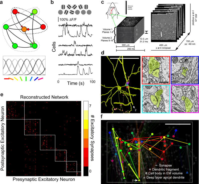
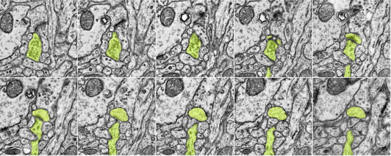
a, Schematic representation of functionally selective connections between excitatory neurons. Excitatory pyramidal cells (large circles) with different preferred orientations provide synaptic input (smaller circles) to one another (bottom: colour code used throughout to indicate stimulus orientation that evokes peak physiological responses). b, Example stimuli (top) and time courses ΔF/F signals from single cells. c, Combined in vivo two-photon calcium imaging followed by electron microscopy (EM). (top left) Schematic of imaging in the awake mouse, targeting the monocular region of the primary visual cortex (largest dotted-outlined region surrounded by higher visual areas). Red arrows represent the visual pathway from eye to visual thalamus to cortex. Serial EM sections (right) were cut orthogonal to the functional imaging planes (left). d, (left) Reconstruction of a layer 2/3 (L2/3) pyramidal neuron (cell 1) presynaptic to a deep layer apical dendrite (cell 2), reconstructed from EM (colour indicates peak stimulus orientation). The thinnest process is the axon, dendrites of the L2/3 neuron are thicker, and the deep layer apical dendrite is rendered with the largest caliber. Dendritic spines were traced only if they participated in connections between reconstructed neurons. Presynaptic boutons (small red spheres with white centers) not connecting this cell pair are semi-transparent. EM micrographs of synapses (right) with similar overlay colours corresponding to the very similar peak orientation preferences for cells 1 and 2. e, Connectivity matrix of 201 excitatory neuronal targets in our network reconstruction with multiple synaptic partners (i.e. degree ≥ 2, no leaf nodes). Colour represents the number of synapses (colour key, right) between pre- and post-synaptic neurons (same neuron order on both ordinate and abscissa). Subnetworks of interconnected neurons (white boxes) detected using a consensus method of Louvain clustering (Q = 0.55 ± .003, mean ± SD)^17,31. f, Network graph of functionally characterized pyramidal neurons and their connections to other excitatory neuronal targets (transparent) viewed coronally. Arrows represent synaptic connections and their shaft thickness is scaled by number of synapses (range: 1–7). Neuronal targets with cell bodies in the EM volume drawn as circles; large caliber apical dendrites that exit the volume (deep layer pyramidal cells) drawn as triangles; and other postsynaptic targets (dendritic fragments) drawn as diamonds. Nodes are positioned by cell body location, synapse location (for dendritic fragments), or, for deep layer apical dendrites, by the deepest position when exiting the volume. Cells labeled 1 and 2 are the same as in (d). Bounding box matches region in Extended Data Fig. 6. Scale bars, d, (left) 100 and (right) 1 μm, f, 100 μm.

We combined in vivo cellular resolution optical imaging with ex vivo EM reconstructions. We measured cellular calcium responses, which reflect the firing of action potentials, using the genetically encoded indicator GCaMP3 to characterize the sensory responses of ~300 × 300 × 200 μm volume of an awake, behaving mouse¹⁰ (Fig. 1b–c). Visual stimuli consisted of drifting sinusoidal gratings of different spatial and temporal frequencies, orientations, and directions (Fig. 1b and Extended Data Fig. 1). In addition to cell bodies in layers 2/3 (L2/3), we measured signals (Extended Data Fig. 2) from large caliber apical dendrites that continued beyond the depth of our imaging volume and had branching morphologies consistent with deep layer pyramidal cells (see Methods). From their responses, we estimated the peak preferred orientation for each cell (Extended Data Fig. 3), with neurons’ visual preferences typically maintained across 12 days of chronic imaging (Extended Data Fig. 1).

After locating the functionally imaged region using vascular landmarks (Extended Data Fig. 4 and Supplementary Video 1), we cut a series of ~3700 serial EM sections, which were imaged with a Transmission Electron Microscope Camera Array⁸ (TEMCA) at ~4 × 4 × 40 nm/voxel. The EM-imaged region spanned 450 × 450 × 150 μm, consisting of ~10 million camera images and ~100 TB of raw data. We traced the processes of excitatory pyramidal neurons located within the middle third of the EM volume (450 × 450 × 50 μm, Supplementary Videos 2 and 3) using software (CATMAID¹⁶) allowing distributed annotation of large image datasets. Teams of trained annotators traced and validated wire-frame models of the dendritic and axonal arbours of neurons selected for reconstruction (chosen because they exhibited visual responses), and located all outgoing synapses along the annotated axons (Fig. 1d, and Extended Data Figs. 5 and 6a). For each synapse, we traced the postsynaptic dendrite centripetally until they reached either the cell body or the boundary of the aligned EM volume (Extended Data Fig. 6b, and Supplementary Data 1–3). We did not retrogradely trace axons providing input to selected neurons because of the lower probability that they originated from cells in the volume. Henceforth, we limit our discussion to the excitatory network from selected pyramidal cells onto spines of excitatory targets.

We first examined the structure of the network broadly, by examining the connectivity of 1278 reconstructed neuronal targets (Table 1). The core of the network (201 neurons connected with more than one other; i.e. degree ≥ 2, no leaf nodes) exhibited a modular structure (Fig. 1e), quantified with a modularity index (Q, which can range from −0.5 to 1) that measures the degree to which a network can be divided into groups, with positive values indicating higher levels of connectivity within than between groups¹⁷. Modularity in the reconstructed network was significantly higher than would be expected by chance (Q_mean = 0.55 ± .003 vs. 0.50 ± .009, mean ± SD, P ≈ 0, Permutation test; Fig. 1e and Extended Data Fig. 7a–d, see Methods) and was not a consequence of higher order motifs (Extended Data Fig. 7). Modularity of the network offers positive evidence for pyramidal cell subnetworks that have previously been inferred from physiological recordings^2,18,19.

Table 1.

Cortical Network Reconstruction

Excitatory neuronal targets	1278
Presynaptic neurons	130
Postsynaptic partners	1228
Deep layer apicals	91
Connected layer 2/3 neurons to deep layer apical pairs	185
Inhibitory neuronal targets	581
Functionally characterized neurons	50
Characterized connected neurons	43
Characterized deep layer apicals	4
Characterized neurons connected to deep layer apicals	20
Functionally characterized connected pairs	29
Unique characterized presynaptics	15
Unique characterized postsynaptics	21
Characterized pairs containing deep layer apicals	8
Unique characterized deep layer apicals in pairs	2
Synapses from characterized neurons	990
Synapses onto inhibitory targets	443
Synapses onto excitatory targets	547
Reconstructed PSDs between characterized pairs	39
Multi-synapse connected pairs	115
Multi-synapse connected pairs with deep layer apicals	62
Multi-synapse connected presynaptic neurons	51
Multi-synapse connected postsynaptic non-deep layer apicals	52
Multi-synapse connected postsynaptic deep layer apicals	41

Numbers of reconstructed neuronal targets (neurons and dendritic fragments), synaptically connected neuron pairs, and synapses analyzed in the EM dataset.

We next examined the degree to which network connectivity reflects the neurons’ sensory properties (Figs. 1f and 2). We focused on 46 L2/3 excitatory neurons and 4 deep layer apical dendrites that showed reproducible responses to visual stimulation (trial correlations p_sftf < 0.05 and p_pos < 0.01, excluding cells with stimulus edge effects, see Methods) and identified their postsynaptic targets. Within the reconstructed network, 43 functionally characterized neurons made 990 synapses, 443 of which were onto inhibitory interneurons and 547 onto other pyramidal cells (Table 1). The large fraction of synapses onto inhibitory neurons is consistent with past observations^8,20 and seems to be a characteristic of L2/3 in the mouse visual cortex. Consistent with physiological studies, connectivity between excitatory neurons was more likely for pairs with similar orientation preferences² (Fig. 2b, P < 0.05, Cochran–Armitage test). This preferential connectivity is not explained by the anatomical arrangement of the cell bodies whose function showed no discernible dependence on distance (Extended Data Fig. 8).

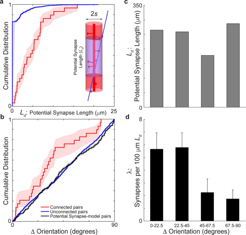
Figure 2. Synaptically connected pyramidal cells predicted by function, over and above proximity.

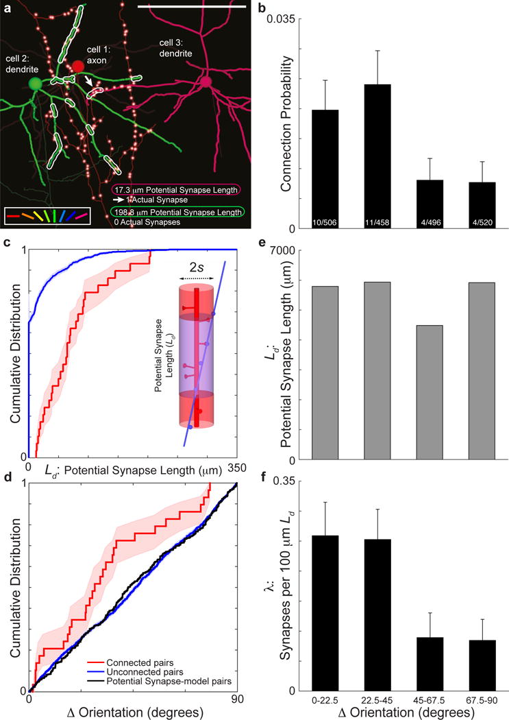
a, Reconstructions of three neurons with examples of potential synapse length (L_d, dotted outlines), which quantifies the dendritic path length of cells 2 and 3 within a maximal spine length (s = 5 μm) of the axon of cell 1. Neurons colour-coded by preferred stimulus orientation (colour key, bottom left; same as Figure 1). Note, the large L_d, but lack of actual synapses between cells 1 and 2 and small L_d between cells 1 and 3 where an actual synapse (arrow) is observed along the L_d. The axon of the postsynaptic cells and dendrites of the presynaptic cell are transparent. Only presynaptic boutons (small red spheres with white centers) from the presynaptic cell are visible. b, Synaptically connected neurons have similar orientation preference. Connection probability as function orientation preference difference across the reconstructed population (P < 0.05, Cochran–Armitage test, n_{connected pairs} = 29, n_{unconnected pairs} = 1951). Bins include pairs of neurons with differences in preferred orientation of 0° to 22.5°, 22.5° to 45°, 45° to 67.5°, and 67.5° to 90°. Fractions at the bottom of bars are the number of connected over unconnected pairs in each bin. c, Synaptically connected neurons have greater potential synapse length. Cumulative distribution of potential synapse length was significantly greater between connected (red line) than unconnected pairs (blue line, P ≈ 0, Permutation test, n_{connected pairs} = 29, n_{unconnected pairs} = 1951, s = 5 μm). Inset: Schematic of a cylinder of length L_d (transparent purple) around the dendrite (red) with a radius (s) equivalent to a maximal spine’s length where the axon (blue) comes within proximity to make a synapse. d, Cumulative distribution of differences in orientation preference was significantly less between connected (red line) than unconnected pairs (blue line, P < 0.05, Permutation test, n_{connected pairs} = 29, n_{unconnected pairs} = 1951) or a model distribution based on potential synapse length (black line, P < 0.05, Permutation test, n_{connected pairs} = 29, n_{unconnected pairs} = 1951). e, Potential synapse length (L_d) is uniform across differences in peak orientation preference between neurons in the model distribution. f, Synapse rate (λ: reconstructed synapses normalized by L_d) decreases with orientation preference difference across the reconstructed population (P < 0.05, Cochran–Armitage test, n_synapses = 39, s = 5 μm). Error bars, b, f, and shaded regions, c-d, represent bootstrapped standard error. Scale bar, a, 100 μm.

Since axons and dendrites of physiologically characterized neurons were traced exhaustively within the volume, we could further evaluate in an unbiased fashion a potential role of axonal and dendritic geometry in specific connectivity. We used a modified measure of potential synapses²¹, which our reconstructions allowed us to compute directly. For each pair of neurons, we quantified potential synapse length, or the length that each dendrite (L_d) traveled within a distance (s) from a given axon, where s can be considered a maximum distance a spine could reach to make a connection (s = 5 μm: Fig. 2a,c; s = 1 μm: Extended Data Fig. 9; see Methods). This helps us formulate a fine-scale version of Peters’ Rule: the hypothesis that the probability of a connection is proportional to the degree of axo-dendritic proximity, independent of other factors. As expected, connected neurons had significantly more L_d than unconnected pairs, that is, their geometry provided more opportunities to make synapses (P ≈ 0, Permutation tests, s = 5 μm, Fig. 2c; s = 1 μm: Extended Data Fig. 9). More interestingly, by considering potential synapse length between pairs with different relative orientations, we found that the neuropil is not functionally organized (P > 0.5, Permutation tests relative to a uniform distribution, s = 5 μm: Fig. 2d, black line, and 2e; s = 1 μm: Extended Data Fig. 9). Therefore, the preferential connectivity (Fig. 2d, red versus blue line, P < 0.05, red versus black line, P < 0.05, Permutation tests; and 2f, P < 0.05, Cochran–Armitage test) between neurons with similar orientation preferences must be the result of mechanisms that take place at the scale of spines: ~1 to 5 μm. Because synapses onto the apical dendrites of deep layer neurons might follow different rules^5,22, we also confirmed statistical significance (P < 0.05, Permutation test, data not shown) with only L2/3 connections.

Recent work suggests that, along with connection probability, the amplitude of excitatory postsynaptic potentials (EPSPs) correlate with receptive field properties¹⁴. Mechanisms underlying the strength of these unitary responses are unknown, for instance whether they are due to multiple synapses, the spatial organization of their synapses, or stronger synapses. Although our sample size was not sufficient to examine the relationship between multiple synapses and function, past work demonstrated that virtually all pyramidal cells are connected by multiple synapses (reviewed in ref. 23). We therefore examined whether synapses connecting pairs of neurons were spatially clustered (Fig. 3a, Fig. 1d,f, thick arrows, and Supplementary Data 3) in a population of fifty-one reconstructed presynaptic neurons connected by multiple synapses onto one or more postsynaptic targets (Table 1). We first computed the synapse rate (λ), or synapses per 100 μm of L_d. As expected, connected neurons coupled by multiple synapses occur more frequently than predicted by chance, having far higher synapses rates for additional synapses compared to a Poisson model (P ≈ 0, Permutation tests relative to a Poisson process with λ, Fig. 3b, compared to Fig. 2f, see Methods). Next, we found that pyramidal neurons were frequently interconnected by multiple synapses arranged close together (17.2 ± 2.9 μm, median ± SE, Fig. 3c) consistent with recent analyses of axon fragments in L5 apical dendrites²⁴ and hippocampus²⁵. A careful analysis of synapse locations considering potential synapse length (L_d), however, shows that closely spaced synapses are not specifically enriched. By comparing the relative magnitude of L_d for regions > 20 μm vs. < 20 μm from each synapse between a pair of neurons, we found that the number of distant synapses correlated (P ≈ 0, Permutation test, n_synapses = 195, Pearson’s r = 0.92) nearly perfectly with the expected value from the pair’s average density of synapses (Fig. 3d, see Methods). That is, axons and dendrites of connected neurons generate multiple synapses when their axon and dendrite remain close, but make additional synapses with an equal rate (λ) elsewhere their processes overlap within our limited volume. This suggests plasticity mechanisms that operate at the cellular rather than dendritic level, but nonetheless leaves open a potential computational role for positioning multiple synapses, which occur both clustered and distributed along the dendritic arbor.

Figure 3. Multiple synapses between neurons are found above chance levels; clustered synapses are frequently observed, but are not specifically enriched.

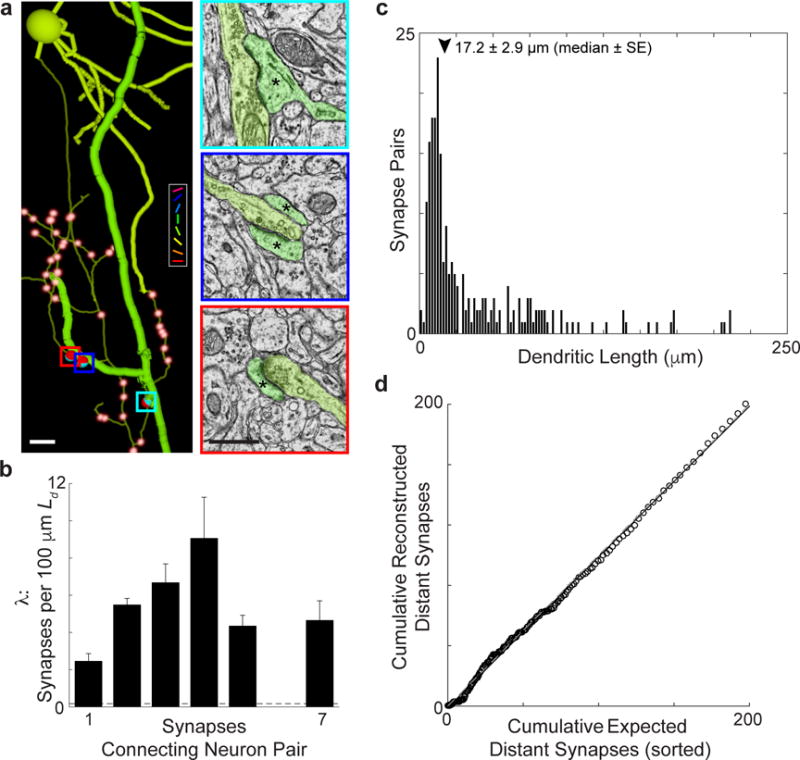
a, Anatomical reconstruction (left) of a L2/3 pyramidal cell presynaptic to a deep layer apical dendrite (thick process) by multiple synapses (right, corresponding colored boxes). Asterisks denote postsynaptic cell. Colour key and synapses not connecting this cell pair are rendered as in Figs. 1 and 2. Of 130 reconstructed presynaptic neurons, 51 had axons making multiple synapses onto individual neuronal targets. b, Synapse rates (λ) normalized by potential synapse length (L_d, s = 5 μm) for neuron pairs connect by 1–7 synapses are significantly higher than expected from a Poisson process with a synapse rate = λ (P ≈ 0, Permutation tests, n_synapses = 292). Dashed line is λ_avg from Fig. 2f. c, Histogram of the dendritic path length between pairs of synapses connecting neurons with multiple synapses. The median distance between synapses connecting neuron pairs was 17.2 ± 2.9 μm (median ± SE, arrowhead). d, Multiple synapses are distributed randomly, with equal tendency to be clustered or distant. The cumulative number of distant (> 20 μm) reconstructed synapses, vs. nearby (< 20 μm), follows the cumulative number expected from a constant synapse rate, based on synapse multiplicity normalized by L_d, for each cell pair. X-axis sorted by expected number of distant synapses; the dashed line is unity. Error bars, b, represent standard error. Scale bars, a, (left) 10 and (right) 1 μm.

Finally, we examined synapse size by measuring postsynaptic density (PSD) area (Fig. 4a), which is proportional to the number of presynaptic vesicles and spine volume²⁶, and may be related to synaptic strength^27–29. We found that PSD areas could be quite large (> 1.0 μm²) for synapses between cells with similar peak orientations (Fig. 4b–c), but were clustered at a smaller size (0.24 ± 0.03 μm², mean ± SE) for the most dissimilar orientations. Connected cells (Fig. 4c, red line) with similar peak orientation preference exhibited larger PSD areas compared to control populations where the orientation selectivity differences or identity of connected cells were shuffled (Fig. 4c, cyan and magenta lines respectively, P < 0.01, Permutation tests). This functionally specific synaptic weighting was significant whether or not spines from apical dendrites were included in the analysis (data not shown). One possibility is that there are multiple classes of synapses, latent connections with smaller synapses, and larger synapses between similarly tuned cells.

Figure 4. Sensory physiology predicts synaptic size.

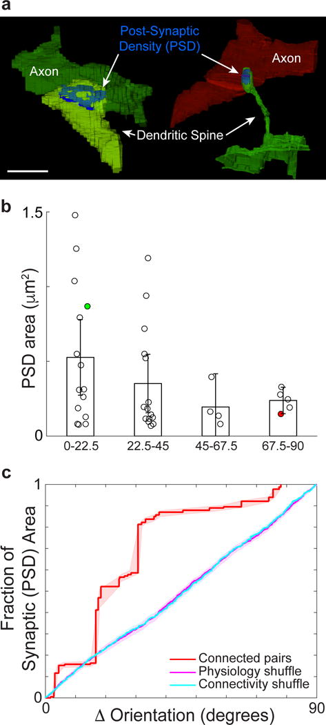
a, Volumetric reconstructions of synapses between functionally characterized cells. Examples of postsynaptic densities (PSDs, blue) for a pair of iso-oriented neurons and for cross-oriented neurons (colour key as in previous figures). b, PSD area decreases as difference in orientation preference increases (examples in (a) labeled green and red respectively; bins: 0° to 22.5°, 22.5° to 45°, 45° to 67.5°, and 67.5° to 90°). c, Cumulative fraction of PSD area accounted for by connections as a function of the difference in orientation preference (red line) is significantly greater than controls (shuffled orientation preference (magenta), or connectivity (cyan), both P < 0.01, Permutation tests, n_synapses = 39). Error bars, b, represent 95% confidence intervals and shaded regions, c, represent bootstrapped standard error. Scale bar, a, 1 μm.

Functional connectomics promises to build bridges between the in vivo activity of neurons, network connectivity, and neuronal structure³⁰. Here, we used this approach to demonstrate five aspects of the excitatory cortical circuit. Independent of physiology, we demonstrate (1) a modular organization network organization that previously had only been inferred indirectly from smaller cortical subnetworks^2,5,18,19, and (2) that multiple synapses between pairs of neurons occur far above chance levels, often closely spaced on the dendrite (<20 μm), although there appears to be no specific mechanism favoring local clustering over widespread spacing. Further, we demonstrate (3) an anatomical substrate of functionally specific connections between neurons, and (4) that this specificity does not result from the spatial arrangement of the neuropil, but instead must operate at the scale of dendritic spines (< 1 – 5 μm). Finally, we show (5) that synapse size correlates with physiology, with larger synapses found between neurons with similar peak orientations. Such specific connectivity is consistent with intracortical amplification of afferent signals, overcoming the strong inhibitory tone in the awake cortex^3,4,15. As methods for automated reconstruction improve, each of these findings will come into greater focus leading to a richer understanding of network structure and function.

Methods

We imaged the primary visual cortex of an awake 9-month-old C57BL/6 male mouse, as described previously^10,13, with a custom-built two-photon microscope¹². Using volumetric in vivo two-photon calcium imaging of a genetically encoded calcium indicator (GCaMP3), we measured the time-resolved responses of a population of identified neurons to a wide array of stimuli including drifting gratings (up to 16 directions, 3 spatial, and 2 temporal frequencies). Following 12 days of imaging calcium responses in the same cohort of neurons, we labeled blood vessels with a tail vein injection (Rhodamine B conjugated dextran) and acquired an in vivo fluorescence volume. The animal’s brain was then prepared for large-scale transmission EM as described previously⁸. 3700 serial sections (< 50 nm thick) were cut and imaged spanning a 450 × 450 × 150 μm volume at 4 × 4 × 40 nm/voxel resolution. Sections representing the middle third of the EM volume were aligned and imported into CATMAID¹⁶ for distributed, online, manual reconstruction and targeted volumes around identified synapses were exported for volumetric segmentation and PSD analysis. EM reconstructed neurons were identified in the in vivo stack by using the blood vessels as landmarks. Apical dendrites originating from deeper neocortical lamina were similarly identified and corresponded by location and branching geometry of their apical tufts. Permutation tests were used in statistical analyses, unless otherwise noted.

Animal preparation

All procedures were conducted in accordance with the ethical guidelines of the NIH and approved by the IACUC at Harvard Medical School. For cranial window implant surgery the mouse was anesthetized with isoflurane (1.2%–2% in 100% O₂). Dexamethasone (3.2 mg/kg, IM) was administered on the day before surgery and atropine (0.2 mg/kg, IP) at the beginning of surgery. Using aseptic technique, we secured a headpost in place using cyanoacrylate, dental acrylic, and C&B Metabond (Parkell), and made a 5 mm craniotomy over the left visual cortex (center: ~2.8 mm lateral, 0.5 mm anterior to lambda) as described previously³². A 5 mm glass cranial window was implanted consisting of an 8 mm coverslip cured to two 5 mm coverslips (Warner #1; total thickness: ~0.5 mm; thickness below skull: ~200 mm) using index-matched adhesive (Norland #71). We secured the window in place using cyanoacrylate and dental acrylic.

We habituated the mouse with water scheduling so that water was delivered only during and immediately after head restraint training. We increased the duration of head restraint sessions over the course of 2 weeks, from 3 min to 2 hr³². We then performed retinotopic mapping of visual cortical areas using widefield intrinsic autofluorescence imaging, measuring autofluorescence produced by blue excitation (470 nm center, 40 nm band, Chroma) through a green/red emission filter (longpass, 500 nm cutoff). We collected images using a CCD camera (Sensicam, Cooke, 344 × 260 pixels spanning 4 × 3 mm; 2 Hz acquisition rate) through a 5X air objective (0.14 NA, Mitituyo) using ImageJ acquisition software. For retinotopic mapping, stimuli were presented at 2–6 retinotopic positions for 10 s each, with 10 s of mean luminance between trials.

GCaMP3 expression was targeted by viral injection. Dexamethasone (3.2 mg/kg, IM) was administered at least 2 hours prior to coverslip removal. The mouse was anesthetized (isoflurane, 1%–1.5%) and the cranial window was sterilized with alcohol and the coverslip removed. We then volume injected (50–100 ml/min, Stoelting) 30–100 nl of a 10:1 mixture of AAV2/1.hSynap.GCaMP3.3.SV40³³ (Penn Vector Core) and 1 mM sulforhodamine-101 (Invitrogen) to visualize the injection. Using the blood vessel pattern observed during widefield imaging as a guide, we made an injection in the posterior part of primary visual cortex at a depth of ~250 μm below the pial surface. After injection, a new cranial window was sealed in place and the mouse recovered.

Visual Stimulation

A 120 Hz LCD monitor (Samsung 2233RZ, 2200) was calibrated at each temporal frequency using a spectrophotometer (Photoresearch PR-650). We confirmed waveforms were sinusoidal by measuring luminance fluctuations of a full-field sinusoidally modulated stimulus (using a photomultiplier tube, Hamamatsu). The monitor was positioned so that the stimulus patch was 21 cm from the contralateral eye. Local 40° Gabor-like circular patches (sigmoidal 10%–90% falloff in 10°) containing either square-wave (for mapping retinotopy with widefield intrinsic autofluorescence and targeting GCaMP3 injections) or sine-wave (for mapping position of receptive fields with two-photon imaging) drifting gratings (80% contrast) were alternated with periods of uniform mean luminance (59 cd/m²). In an effort to increase the population of responsive cells and explore receptive field parameters we presented gratings of varying directions at multiple spatial and temporal frequencies or at different positions in the visual field. We presented either 8 directions at 3 spatial frequencies (0.06, 0.12, and 0.24 cycles per degree (cpd)) and 2 temporal frequencies (2 and 8 Hz), 16 directions at 2 spatial frequencies (0.04 and 0.16 cpd) and 2 temporal frequencies (2 and 8 Hz), 8 directions at 6 positions, or 16 directions at 4 positions (45–115° eccentricity and −5–25° elevation), for a total of 64 stimulus types plus 10% blank trials. Stimuli were centered on the location eliciting maximum calcium responses in the imaged field (monocular cortex), which most effectively drove responses in the population for experiments that did not vary stimulus position. All stimuli in a given protocol were presented in a pseudo-random order (sampling without replacement), and presented 3 times per volume experiment with 2–4 experiments per volume per day.

Two-Photon Calcium Imaging

Imaging was performed with a custom-designed two-photon laser-scanning microscope¹². Excitation light from a Mai Tai HP DeepSee laser (Spectra-Physics) with dispersion compensation was directed into a modulator (Conoptics) and a beam expander (Edmund Optics). The expanded beam was raster scanned into the brain with a resonant (4 kHz, Electro-Optical Products) and a conventional galvanometer (Galvoline) (240 line frames, bidirectional, 31 Hz) through a 0.8 numerical aperture (NA) 16X objective lens (Nikon). Emitted photons were directed through a green filter (center: 542 nm; band: 50 nm; Semrock) onto GaAsP photomultipliers (no cooling, 50 μA protection circuit, H7422P-40MOD, Hamamatsu). The photomultiplier signals were amplified (DHPCA-100, Femto), and low-pass filtered (cutoff frequency = ~700 kHz). These and the mirror driver signals were acquired at 3.3 MHz using a multifunction data acquisition board (PCI-6115, National Instruments). Images were reconstructed in MATLAB (MathWorks) and continuously streamed onto a RAID array. Microscope control was also performed in MATLAB using an analog output board (PCI-6711, National Instruments). The laser’s dispersion compensation was adjusted to maximize collected fluorescence.

A piezoelectric objective translator on the microscope enabled imaging multiple 300 × 300 × 100 μm volumes with 8 planes at 4 Hz separated by ~12.5 μm allowing us to capture the response properties of many cells through the depth of L2/3. The imaged field of view was 200–300 μm on a side at resolution of 0.8–1.2 μm/pixel (dwell-time ~2.7 μs). GCaMP3 was excited at 920 nm. Laser power was automatically adjusted as a function of imaging depth at the modulator with power exiting the objective ranging from 30–60 mW.

During imaging, the mouse was placed on 6” diameter foam ball that could spin noiselessly on an axel (Plasteel). We monitored trackball revolutions using a custom photodetector circuit and recorded eye movements using an IR-CCD camera (Sony xc-ei50; 30 Hz) and infrared illumination (720–2750 nm bandpass filter, Edmund). Visual stimuli were presented for 4 s with 4 s of mean luminance between trials. Recording sessions were 2–6 hr in duration.

Use of the genetically encoded calcium indicator GCaMP3, permitted recording from the same neurons over multiple days with the selectivity of calcium signals stable over several days of imaging (Extended Data Fig. 1)^32,34,35. Within this volume we obtained calcium signals from cell bodies of superficial layer (L2/3) neurons and large caliber apical dendrites that continued beyond the depth of our imaging volume and had branching morphologies consistent with deep layer pyramidal cells. These were likely from L5 neurons because of their large caliber, and because most L6 pyramidal cells do not project their apical dendrites more superficially than L4^36,37. The calcium signals from these deep layer apical dendrites stem from either forward-^38,39 or back-propagating action potentials⁴⁰, are consistent across days (Extended Data Fig. 1) and along the length of the deep layer apical dendritic trunks (Extended Data Fig. 2), and therefore most likely reflect the response properties of the soma. We relocated the cohort of neurons daily by using the vasculature’s negative staining as fiducial landmarks. For the final in vivo imaging session, we injected the tail vein with a fluorescent dye to label blood vessels (Rhodamine B isothicyanate-Dextran (MW ~70k), 5% v/v, Sigma) and acquired a fluorescence stack to correspond the calcium-imaged neurons in vivo with their identities in the EM volume ex vivo⁸ (see below, and Extended Data Fig. 4).

EM material preparation

Following in vivo two-photon imaging the animal was perfused transcardially (2% formaldehyde/2.5% glutaraldehyde in 0.1M Cacodylate buffer with 0.04% CaCl₂) and the brain was processed for serial-section TEM. 200 μm thick coronal vibratome sections were cut, post-fixed, and en bloc stained with 1% osmium tetroxide/1.5% potassium ferrocyanide followed by 1% uranyl acetate, dehydrated with a graded ethanol series, and embedded in resin (TAAB 812 Epon, Canemco). We located the calcium-imaged region by matching vasculature between in vivo fluorescence and serial thick (1 μm) toluidine blue (EMS) sections cut from an adjacent vibratome sections, then cut ~3700 serial (<50 nm) sections on an ultramicrotome (Leica UC7) using a 35 degree diamond knife (EMS-Diatome) and manually collected sections on 1×2 mm dot-notch slot grids (Synaptek) that were coated with a pale gold Pioloform (Ted Pella) support film, carbon coated, and glow-discharged. Following section pickup, we post-stained grids with uranyl acetate and lead citrate.

Large-scale TEM imaging, alignment, and correspondence

Using the custom-built Transmission Electron Microscope Camera Array (TEMCA)⁸ we imaged the ~3700 section series, targeting a ~450 × 450 μm region for each section (Fig. 1c). Acquired at 4 nm/pixel in plane, this amounted to ~100 terabytes of raw data to date comprising 30 million cubic microns of brain and > 10 million (4000 × 2672 pixel) camera images. Magnification at the scope was 2000x, accelerating potential was 120 kV, and beam current was ~90 microamperes through a tungsten filament. Images suitable for circuit reconstruction were acquired at a net rate of 5–8 MPix/s. Approximately the middle third of the series (sections 2281–3154) was aligned using open source software developed at Pittsburgh Supercomputing Center (AlignTK)⁸ and imported into CATMAID¹⁶ for distributed online visualization and segmentation. Within the analyzed EM series there were 51 missing sections. Nineteen were single section losses. There were 2 instances each of missing 2, 3, and 4; and 1 instance each of missing 6 or 8 consecutive sections near the series boundaries. Folds, staining artifacts, and some times cracks occurred during section processing, but were typically isolated to edges of our large sections and therefore did not usually interfere manual segmentation. To find the correspondence between the cells imaged in vivo with those in the EM data set, a global 3-D affine alignment was used with fiducial landmarks manually specified at successively finer scales of vasculature and then cell bodies to re-locate the calcium-imaged neurons in the EM-imaged volume (Extended Data Fig. 4). Apical dendrites arising from deep layer (putative L5) pyramidal neurons were identified by their characteristic morphology^36,41,42 (also see below). Their correspondence was facilitated by the unique branching patterns of their apical tufts and those that could not be unambiguously identified were not included in the functional analysis.

Reconstruction and verification

We first traced the axonal and dendritic arbours of the functionally characterized neurons in the EM dataset by manually placing a series of marker points down the midline of each process to generate a skeletonized model of the arbours using CATMAID¹⁶ (Figs. 1d, 2a, 3a, Extended Data Fig. 6, Supplementary Data 1–3). We identified synapses using classical criteria⁴². For each synapse on the axon of a functionally characterized cell, dendrites of postsynaptic excitatory neurons were traced either to the boundaries of the aligned volume or centripetally back to the cell body⁸. We identified deep layer apical dendrites of (putative L5) pyramidal cells by their large caliber, high spine density, and their continuation beyond the bottom border of the EM volume, which spans from the pial surface through L4. For each neuronal target reconstruction included in the analysis, a second independent annotator verified the tracing by working backwards from the most distal end of every process. An additional round of validation was done for each synapse between functionally characterized cells where a third annotator who had not previously traced the pre- or post-synaptic process, independently verified the anatomical connectivity blind to previous tracing work. We began this independent round of validation at each synapse and traced the pre- and postsynaptic processes centripetally. If the initial reconstruction and subsequent verification of the reconstruction diverged, that connection and the segmentation work distal from the point of divergence was excluded from further analysis. EM reconstruction and validation was performed blind to cells’ functional characteristics and targeted cells were initially assigned to individual annotators pseudorandomly weighted by tracing productivity.

We performed targeted volumetric reconstructions of synapses connecting functionally characterized cells by developing tools to interface with CATMAID cutout, locally align, and catalogue volumes of interest based on location (Fig. 4a; e.g. 400 pix × 400 pix × 41 sections or 1.6 × 1.6 × 1.64 μm volumes centered on synapses represented by CATMAID connectors). Presynaptic boutons, postsynaptic spines, their parent axons and dendrites, and postsynaptic density (PSD) areas were manually segmented with itk-SNAP (http://www.itksnap.org/). PSD areas were calculated as described previously⁴³ with obliquely cut or en face synapse areas measured using their maximum z-projection. En face or obliquely cut synapses were identified by serial sections that starkly transitioned from a clear presynaptic specialization hosting a vesicle pool, to a distinctly different postsynaptic cell, typically with an intervening section of electron dense area representing the postsynaptic density and/or synaptic cleft (e.g. Extended Data Fig. 5).

Data analysis

In vivo calcium imaging data was analyzed in MATLAB and ImageJ (NIH) as described previously^12,13. To correct for motion along the imaged plane (x–y motion), the stack for each imaging plane was registered to the average field of view using TurboReg⁴⁴. A 5 pixel border at each edge of the field of view was ignored to eliminate registration artifacts. Masks for analyzing fluorescence signal from neurons were manually generated corresponding to cells in the EM volume, registered to the in vivo anatomical fluorescence stack, and to individual physiological imaging planes. Time courses of cells spanning multiple physiological imaging planes were weighted by dwell time in each plane and averaged across planes. Evoked responses for each EM identified cells were measured for each stimulation epoch as the difference in fractional fluorescence (% ΔF/F₀) between the 5 s after and the 2.5 s before stimulus onset (pre-stimulus activity), and averaged across stimulus repetitions. We quantified visual responsiveness of each cell by calculating the average Pearson correlation coefficient of the responses to all stimuli across repetitions (average trial-to-trial correlation). We defined the significance of visual responses as the probability (p-value) that the observed trial-to-trial correlation is larger than the correlation obtained from a full random permutation of the data for spatial and temporal frequency experiments (p_sftf < 0.05) and experiments where stimulus position was varied (p_pos< 0.01). In retinotopic experiments designed to increase the number of characterized neurons, we found cells that did not reliably respond to stimuli ±20° from the center of the display. These cells that either had receptive fields smaller than our stimuli or stimuli were positioned at the at the edge of their receptive fields. We considered these cells as potentially driven by stimulus edge effects and therefore excluded such experiments from further analysis. To estimate the preferred orientation, direction, and spatiotemporal frequency, we modeled responses with a combination of a multivariate Gaussian with spatial frequency (x and y, deg), temporal frequency (Hz) and position (x and y, deg) as independent dimensions, a constant gain factor, and a static exponent. We fit the model to data using a large-scale nonlinear optimization algorithm (Trust Region Reflective, MATLAB Optimization Toolbox, MathWorks Inc.), generating multiple fits from randomly selected starting points and selected the best fit (least-square criterion). The quality of model fits was inspected visually for all neurons included in the data set.

EM connectivity was analyzed using custom written software in MATLAB and Python. Connectivity analysis that did not utilize functional information (Figs. 1e and 3, Extended Data Fig. 7) started with the entire population of excitatory neuronal targets in the reconstructed network. Network modularity and neuron connectivity motifs (Fig. 1e and Extended Data Fig. 7) were analyzed with code modified from the Brain Connectivity Toolbox⁴⁵. We used an implementation of the Louvain method¹⁷ followed by consensus portioning⁴⁶ for weighted and directed graphs to detect communities, or interconnected pyramidal neuron targets, from our EM reconstructed network purely by anatomical connectivity. For this analysis we included only the 201 traced neurons having multiple synaptic partners (degree ≥ 2). The number of synapses reconstructed between neurons was used as weights for all analyses. Modularity Q was given by the standard equation:

$$Q=\frac{1}{l}{\displaystyle \sum _{i,j\in N}\left[a_{ij}-\frac{k_i^{\mathit{out}}{k}_j^{\mathit{in}}}{l}\right]\delta \left(m_i,m_j\right)}$$

where l is the total number of edges, given by

$$l={\displaystyle \sum _{i,j\in N}{a}_{ij}}$$

where N is the total set of nodes, a_ij is the (i,j) element of the weighted adjacency matrix, δ(m_i,m_j) is 1 if i and j are in the same community and 0 otherwise, $k_j^{\mathit{in}}$ and $k_{\mathrm{i}}^{\text{out}}$ are the in and out degrees of the j^th and i^th nodes respectively, calculated by

$k_j^{\mathit{in}}={\displaystyle \sum }_{\mathrm{i}\in \mathrm{N}}{a}_{ij}{k}_i^{\mathit{out}}={\displaystyle \sum }_{\mathrm{j}\in \mathrm{N}}{a}_{ij}$

To generate null models of connectivity matrices for hypothesis testing, we shuffled the reconstructed adjacency conditioned on our sample degree, weight and strength distributions (Extended Data Fig. 7)^31,47.

Analysis of connectivity with neuronal function restricted our sample population to those cell pairs where both pre- and post-synaptic cells were functionally characterized. For orientation tuning (Figs. 1d,f, 2, 4a–c, Extended Data Figs. 5–6, 8–9), between 50 neurons, there were 29 connected pairs. On average, we detected 1.3 synapses per connected pair where we measured orientation selectivity for both cells. We varied retinotopic position and spatial and temporal frequencies of the grating stimulus with the goal of improved measurement of orientation preference for more cells. The sensory physiology of a subset of cells were simultaneously recorded across multiple stimulus parameters. These 120 cells were used for signal correlation analysis (Extended Data Fig. 10).

Potential synapse length (L_d) represents the degree to which pairs of neurons’ axonal and dendritic arbors come sufficiently close to make a synapse (Fig. 2a,c–f, 3b,d, Extended Data Figs. 9–10). For excitatory pyramidal cells, we computed this length of potential synaptic connectivity between all pairs by first resampling the dendritic and axonal arbour skeletons to a maximum segment length of 40 nm (the average thickness of the EM sections) and summing the length of all dendrite segments within a maximum spine length distance of the axon (s = 5 μm: Fig. 2, 3 and Extended Data Fig. 10; s = 1 μm: Extended Data Fig. 9). We use s = 5 μm based the longest spine connecting functionally connected neurons (~ 5 μm).

Analysis of neurons connected by multiple synapses (Fig. 3) was not restricted to cell pairs where both pre and post-synaptic cells were physiologically characterized. This population included 137 neurons connected by 267 synapses in 115 multi-synapse cell pairs whose axonal and dendritic arbours were traced exhaustively in the aligned volume. As a comparison population, we used 25 unique pairs connected by one synapse from the functionally characterized population described above, because they were also reconstructed throughout the aligned volume. To examine whether poly-synaptic connectivity occurs greater than random, we first computed a population average synapse rate (λ_avg) normalized by potential synapse length, by dividing the total number of synapses reconstructed from the set of 50 functionally characterized neurons by their total pairwise L_d. We next compared λ for individual neuron pairs each connected by different numbers of synapses (Fig. 3b). This was used to assess whether multiple synapses occurred more often than predicted from a simple Poisson model.

We examined the frequency of clustered vs. distant synapses by comparing synapse pairs that were separated by > 20 μm or < 20 μm. For each synapse from each pair of neurons connected by n synapses, we computed the total L_d within 20 μm or beyond 20 μm from that synapse. We then took the fraction of the overlap beyond 20 μm:

$$L_d(>\mathit{20}\mu m)/[L_d(<\mathit{20}\mu m)+L_d(>\mathit{20}\mu m)]$$

as the expected probability that each of the (n − 1) other synapses will occur > 20 μm away. The expected number of distant synapse was taken as (n − 1) times the fraction of overlap beyond 20 μm, which was compared with the actual number of distant synapses observed (Fig. 3d).

3-D renderings were generated using Blender (http://www.blender.org/) (Figs. 1d, 2a, 3a, Extended Data Fig. 6, Supplementary Data 1–3), Imaris (Bitplane) (Extended Data Fig. 4 and Supplemental Video 1), and itk-SNAP (Fig. 4a). Cytoscape (http://www.cytoscape.org/) was used for network graph layouts (Figs. 1f).

Statistics

Statistical methods were not used to predetermine sample sizes. Statistical comparisons between sample distributions were done with Permutation tests (i.e. Monte Carlo-based Randomization tests) unless otherwise noted. Permutation test were ideal as we do not assume the underlying distributions are normal, nor need the observations to be independent. For Permutation tests, we computed the incidence of differences between means or Pearson’s linear correlation coefficient of randomly drawn samples from combined sample distributions exceeding the empirical difference (Figs. 2b–d,f, 4c, and Extended Data Figs. 7b, 9a–b, 10c–d). Cochran-Armitage two-sided tests for trend were used on proportional binned data with linear weights (Figs. 2b,f). Standard errors were calculated from bootstrapped sample distributions. For cumulative distributions (Figs. 2c–d, 4c, and Extended Data Figs. 9a–b, 10c–d), we repeatedly resampled by randomly drawing with replacement from the sample distribution the number of observed values 1,000–10,000 times and extracted the standard deviation at each step of the empirical CDF. For binned data (Figs. 2b,f, and Extended Data Figs. 9d), each resampled distribution was binned and the standard deviation was computed from the resampled probabilities or rates within each bin.

Extended Data

Extended Data Figure 1. Sensory physiology is maintained over days.

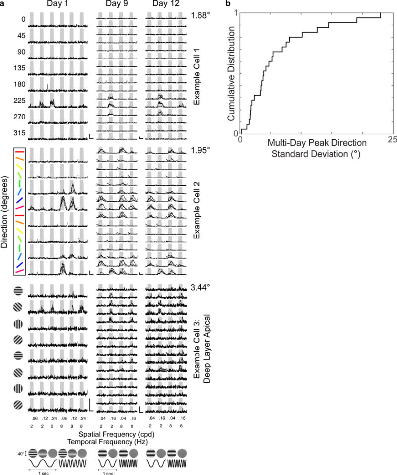
a, Visually evoked calcium responses are maintained across days. Three example neurons (rows) on the first, ninth, and twelfth day (columns) of in vivo two-photon calcium imaging. Three individual trial responses (black lines) of 8 directions, 3 spatial and 2 temporal frequencies (left column, day 1); or 16 directions, 2 spatial and 2 temporal frequencies (middle and right rows, days 9 and 12). Scale bars, 100% ΔF/F and 4 seconds. Standard deviation of preferred direction across days for each neuron is to the upper right of activity matrices. b, Neurons direction selectivity is stable over days. Cumulative distribution of standard deviation of peak preferred direction (4.1° ± 1.7°, median ± SE) across days for 25 neurons measured over multiple days.

Extended Data Figure 2. Deep layer apical responses are likely suprathreshold reflecting activity at the soma.

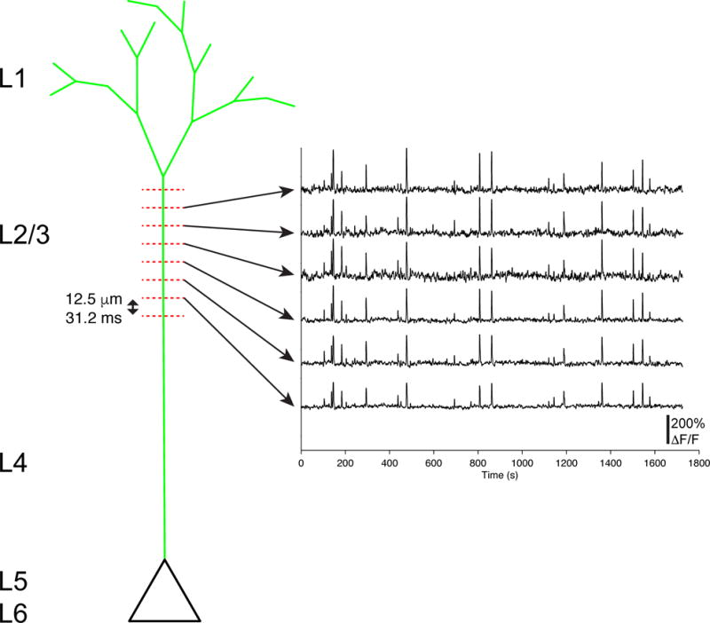
Example ΔF/F time courses from a deep layer apical dendrite optically sectioned in vivo across 6–8 planes. Note, activity is correlated across depth and relatively stable over days (Extended Data Fig. 1).

Extended Data Figure 3. Distribution of orientation and direction tuned cells.

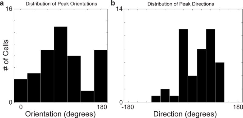
Histograms of functionally characterized cells with measured a, peak orientation and b, direction preference.

Extended Data Figure 4. In vivo to EM correspondence of neuronal targets.

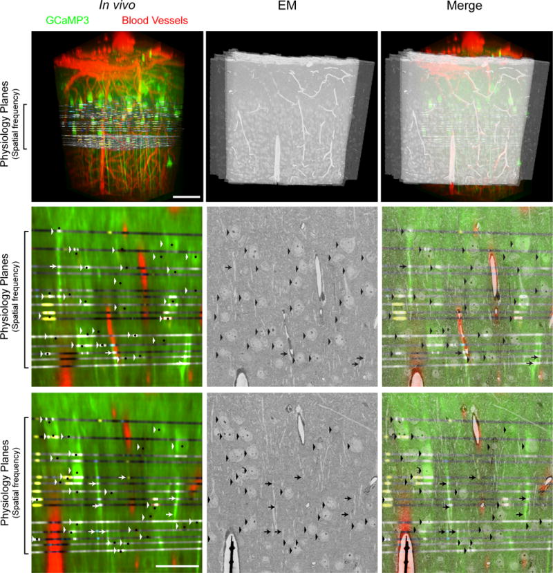
(top row) Volumetric projections of the aligned in vivo and EM imaged volumes. Physiology planes were acquired horizontally and EM sections cut frontally (coronally) from the brain. Interdigitated physiology planes are from 2 representative volumetrically scanned experiments stacked atop one another in space (Fig. 1c) so as to span from the border of L1 and L2 through the depth of L2/3. Scale bar, 100 μm. (middle and bottom rows) Re-sliced planes through the in vivo volume corresponding to EM sections. Arrowheads indicate matching cell bodies, and arrows deep layer (putative L5) apical dendrites. Small black dots mark the centers of cell bodies corresponding principally to nuclei where calcium indicator fluorescence is typically excluded. Scale bar, 50 μm.

Extended Data Figure 5. En face synapse example.

Serial sections from an obliquely cut synapse (Fig. 1d, top right, same scale). Color overlays correspond to peak orientation preference (colour key, same as Fig. 1a, bottom).

Extended Data Figure 6. Network reconstruction.

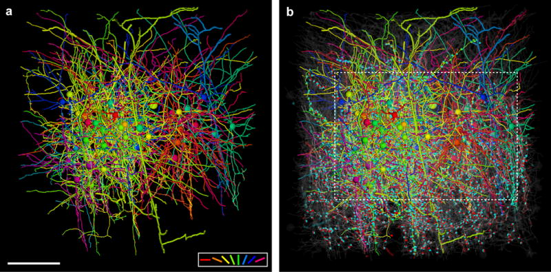
3-D rendering of dendrites and axons, cell bodies (large spheres), and synapses (small spheres) of a, 50 functionally characterized neurons reconstructed in the EM volume. Cell bodies, dendrites, axons, and synapses colour coded by peak preferred stimulus orientation (colour key, bottom right). Axons are the thinnest processes, dendrites of L2/3 neurons are thicker, and deep layer apical dendrites are rendered with the largest caliber. Dendritic spines were traced only if they participated in connections between reconstructed neurons. b, ~1800 additional neuronal targets reconstructed in the EM volume (transparent gray). Input and output synapses are coloured cyan and red respectively when orientation selectivity was not known. Bounding box matches region in Fig. 1f. Scale bar, 150 μm.

Extended Data Figure 7. Network modularity is significantly non-random.

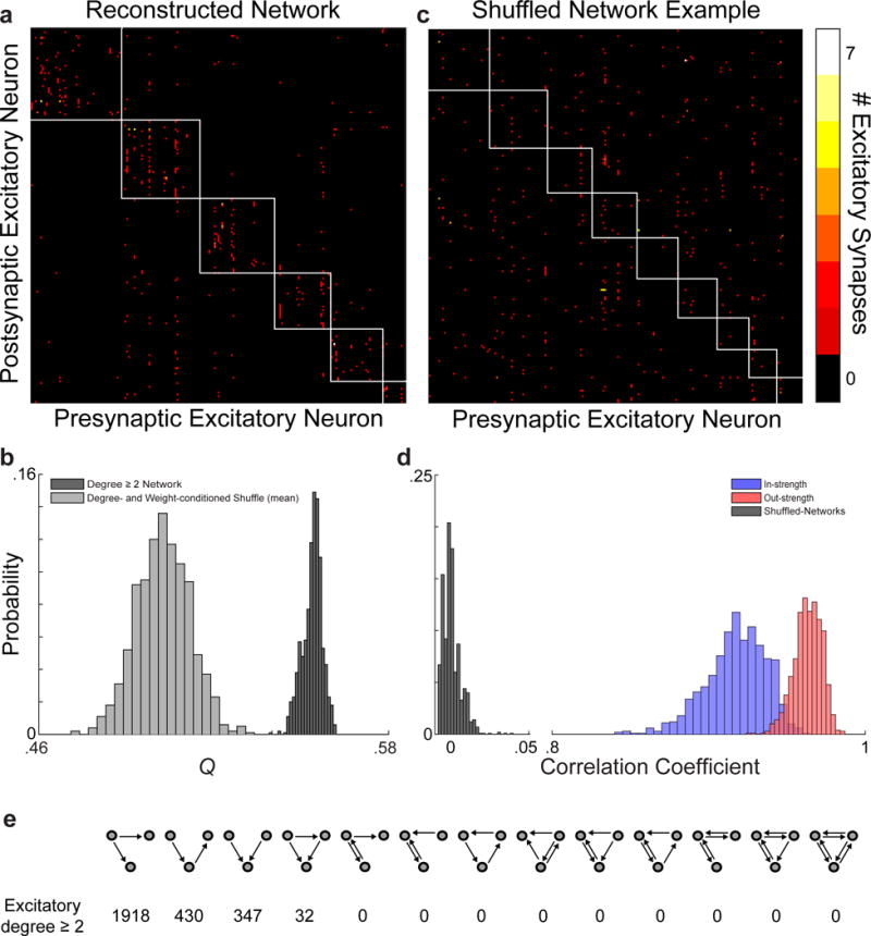
a, Connectivity matrix of 201 excitatory neuronal targets in our network reconstruction with multiple synaptic partners (i.e. degree ≥ 2, no leaf nodes, same as Fig. 1e). Colour represents the number of synapses (colour key, (c) right) between pre- and post-synaptic neurons (same neuron order on both ordinate and abscissa). Subnetworks of interconnected neurons (white boxes) detected using a consensus method of Louvain clustering^17,31. b, Modularity (Q) of the reconstructed network is significantly greater than null models with degree, weight, and strength preserved. Histograms of the modularity values for the reconstructed network (dark gray, Q_mean = 0.55 ± .003, mean ± SD, computed 1000 times) is significantly greater than for the Q_mean of shuffled null models (light gray, Q_mean = 0.50 ± .009, mean ± SD, P ≈ 0, Permutation test, k_shuffles = 1000). c, Example of the shuffled connectivity matrix with a Q closest to the mean of the shuffled distribution with clustering (white boxes) computed as in (a). d, Null models are well-shuffled, while approximating connection input and output strengths. Histograms of correlation coefficients between the reconstructed network and the null models’ in- (blue: .92 ± .02, mean ± SD) and out- (red: 96 ± .01, mean ± SD) strength and connectivity matrix (gray: 9.1×10⁻⁴ ± .01, mean ± SD). e, Occurrences of three neuron connectivity motifs found in the reconstructed network between excitatory neuronal targets.

Extended Data Figure 8. Cell bodies are functionally intermingled.

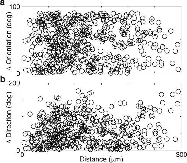
Differences in a, peak orientation and b, direction preference between neuron pairs plotted against the distance between their cell bodies. Uniform distributions of functional versus spatial distance suggest a salt and pepper intermingling of neuronal cell bodies across functional properties.

Extended Data Figure 9. Axons and dendrites are functionally intermingled at shorter length scales.

Uniform functional diversity and prediction of connectivity at finer length scales suggest a salt and pepper intermingling of axons and dendrites. (a-d) same as Fig. 2c–f for s = 1 μm. Significance tests: (a) P ≈ 0, Permutation test, n_{connected pairs} = 29, n_{unconnected pairs} = 1951. (b) Between connected (red line) and unconnected pairs (blue line, P < 0.05, Permutation test, n_{connected pairs} = 29, n_{unconnected pairs} = 1951) or a model distribution based on potential synapse length (black line, P < 0.01, Permutation test, n_{connected pairs} = 29, n_{unconnected pairs} = 1951). Shaded regions, a-b, and error bars, d, represent bootstrapped standard error.

Extended Data Figure 10. Connectivity is not predicted by residual signal correlation after removal of orientation preference.

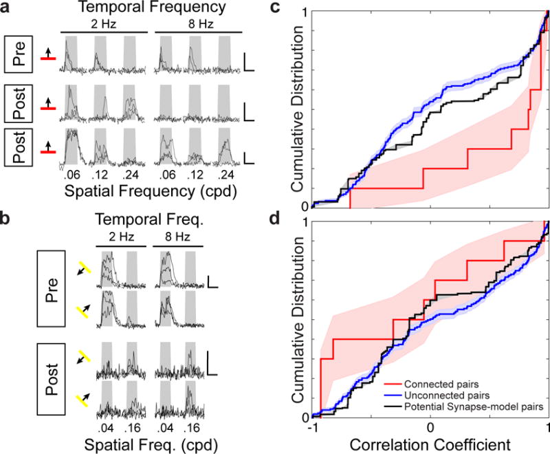
(a–b), Example activity (ΔF/F individual trial time courses) for connected neurons from experiments varying direction, spatial and temporal frequencies of grating stimuli. a, Presynaptic cell (top row) and two of its postsynaptic partners’ (middle and bottom rows) for 3 spatial and 2 temporal frequencies and one orientation (orientation tuning was virtually identical). b, Presynaptic cell (top) and a postsynaptic deep layer apical dendrite’s (bottom) responses to 2 spatial and 2 temporal frequencies, and 2 directions, (again, orientation tuning was virtually identical). Gray window delineates time of stimulus presentation. Scale bars, 100% ΔF/F and 4 seconds. c, Cumulative distribution of signal correlations from simultaneously measured cells was significantly greater between connected than unconnected pairs (P < 0.01, Permutation test, n_{connected pairs} = 10, n_{unconnected pairs} = 426) or a model distribution based on potential synaptic connectivity (P < 0.05, Permutation test). d, After averaging over orientations, the cumulative distribution of signal correlations was similar between connected and unconnected pairs (P > 0.14, Permutation test, n_{connected pairs} = 10, n_{unconnected pairs} = 426) and a model distribution based on potential synaptic connectivity (P > 0.25, Permutation test, n_{connected pairs} = 10, n_{unconnected pairs} = 426). Shaded regions, c-d, represent bootstrapped standard error.

References

- 1.Harris KD, Mrsic-Flogel TD. Cortical connectivity and sensory coding. Nature. 2013;503:51–58. doi: 10.1038/nature12654. [DOI] [PubMed] [Google Scholar]
- 2.Ko H, et al. Functional specificity of local synaptic connections in neocortical networks. Nature. 2011 doi: 10.1038/nature09880. [DOI] [PMC free article] [PubMed] [Google Scholar]
- 3.Li YT, Ibrahim LA, Liu BH, Zhang LI, Tao HW. Linear transformation of thalamocortical input by intracortical excitation. Nat Neurosci. 2013;16:1324–1330. doi: 10.1038/nn.3494. [DOI] [PMC free article] [PubMed] [Google Scholar]
- 4.Lien AD, Scanziani M. Tuned thalamic excitation is amplified by visual cortical circuits. Nat Neurosci. 2013;16:1315–1323. doi: 10.1038/nn.3488. [DOI] [PMC free article] [PubMed] [Google Scholar]
- 5.Wertz A, et al. Single-cell-initiated monosynaptic tracing reveals layer-specific cortical network modules. Science. 2015;349:70–74. doi: 10.1126/science.aab1687. [DOI] [PubMed] [Google Scholar]
- 6.Niell CM, Stryker MP. Highly selective receptive fields in mouse visual cortex. J Neurosci. 2008;28:7520–7536. doi: 10.1523/JNEUROSCI.0623-08.2008. [DOI] [PMC free article] [PubMed] [Google Scholar]
- 7.Kerlin AM, Andermann ML, Berezovskii VK, Reid RC. Broadly tuned response properties of diverse inhibitory neuron subtypes in mouse visual cortex. Neuron. 2010;67:858–871. doi: 10.1016/j.neuron.2010.08.002. [DOI] [PMC free article] [PubMed] [Google Scholar]
- 8.Bock DD, et al. Network anatomy and in vivo physiology of visual cortical neurons. Nature. 2011;471:177–182. doi: 10.1038/nature09802. [DOI] [PMC free article] [PubMed] [Google Scholar]
- 9.Hofer SB, et al. Differential connectivity and response dynamics of excitatory and inhibitory neurons in visual cortex. Nat Neurosci. 2011;14:1045–1052. doi: 10.1038/nn.2876. [DOI] [PMC free article] [PubMed] [Google Scholar]
- 10.Andermann ML, Kerlin AM, Roumis DK, Glickfeld LL, Reid RC. Functional specialization of mouse higher visual cortical areas. Neuron. 2011;72:1025–1039. doi: 10.1016/j.neuron.2011.11.013. [DOI] [PMC free article] [PubMed] [Google Scholar]
- 11.Marshel JH, Garrett ME, Nauhaus I, Callaway EM. Functional specialization of seven mouse visual cortical areas. Neuron. 2011;72:1040–1054. doi: 10.1016/j.neuron.2011.12.004. [DOI] [PMC free article] [PubMed] [Google Scholar]
- 12.Bonin V, Histed MH, Yurgenson S, Reid RC. Local diversity and fine-scale organization of receptive fields in mouse visual cortex. J Neurosci. 2011;31:18506–18521. doi: 10.1523/JNEUROSCI.2974-11.2011. [DOI] [PMC free article] [PubMed] [Google Scholar]
- 13.Glickfeld LL, Andermann ML, Bonin V, Reid RC. Cortico-cortical projections in mouse visual cortex are functionally target specific. Nat Neurosci. 2013 doi: 10.1038/nn.3300. [DOI] [PMC free article] [PubMed] [Google Scholar]
- 14.Cossell L, et al. Functional organization of excitatory synaptic strength in primary visual cortex. Nature. 2015;518:399–403. doi: 10.1038/nature14182. [DOI] [PMC free article] [PubMed] [Google Scholar]
- 15.Reinhold K, Lien AD, Scanziani M. Distinct recurrent versus afferent dynamics in cortical visual processing. Nat Neurosci. 2015;18:1789–1797. doi: 10.1038/nn.4153. [DOI] [PubMed] [Google Scholar]
- 16.Saalfeld S, Cardona A, Hartenstein V, Tomancak P. CATMAID: collaborative annotation toolkit for massive amounts of image data. Bioinformatics. 2009;25:1984–1986. doi: 10.1093/bioinformatics/btp266. [DOI] [PMC free article] [PubMed] [Google Scholar]
- 17.Blondel VD, Guillaume JL, Lambiotte R, Lefebvre E. Fast unfolding of communities in large networks. J Stat Mech Theor Exp. 2008;2008:P10008. [Google Scholar]
- 18.Song S, Sjostrom PJ, Reigl M, Nelson S, Chklovskii DB. Highly nonrandom features of synaptic connectivity in local cortical circuits. PLoS Biol. 2005;3:e68. doi: 10.1371/journal.pbio.0030068. [DOI] [PMC free article] [PubMed] [Google Scholar]
- 19.Yoshimura Y, Dantzker JL, Callaway EM. Excitatory cortical neurons form fine-scale functional networks. Nature. 2005;433:868–873. doi: 10.1038/nature03252. [DOI] [PubMed] [Google Scholar]
- 20.Bopp R, Macarico da Costa N, Kampa BM, Martin KA, Roth MM. Pyramidal Cells Make Specific Connections onto Smooth (GABAergic) Neurons in Mouse Visual Cortex. PLoS Biol. 2014;12:e1001932. doi: 10.1371/journal.pbio.1001932. [DOI] [PMC free article] [PubMed] [Google Scholar]
- 21.Stepanyants A, Hof PR, Chklovskii DB. Geometry and structural plasticity of synaptic connectivity. Neuron. 6529;34:275–288. doi: 10.1016/s0896-6273(02)00652-9. [DOI] [PubMed] [Google Scholar]
- 22.Kampa BM, Letzkus JJ, Stuart GJ. Cortical feed-forward networks for binding different streams of sensory information. Nat Neurosci. 2006;9:1472–1473. doi: 10.1038/nn1798. [DOI] [PubMed] [Google Scholar]
- 23.Reimann MW, King JG, Muller EB, Ramaswamy S, Markram H. An algorithm to predict the connectome of neural microcircuits. Front Comput Neurosci. 2015;9:120. doi: 10.3389/fncom.2015.00120. [DOI] [PMC free article] [PubMed] [Google Scholar]
- 24.Kasthuri N, et al. Saturated Reconstruction of a Volume of Neocortex. Cell. 2015;162:648–661. doi: 10.1016/j.cell.2015.06.054. [DOI] [PubMed] [Google Scholar]
- 25.Bartol TM, et al. Nanoconnectomic upper bound on the variability of synaptic plasticity. Elife. 2015;4 doi: 10.7554/eLife.10778. [DOI] [PMC free article] [PubMed] [Google Scholar]
- 26.Harris KM, Stevens JK. Dendritic spines of CA 1 pyramidal cells in the rat hippocampus: serial electron microscopy with reference to their biophysical characteristics. J Neurosci. 1989;9:2982–2997. doi: 10.1523/JNEUROSCI.09-08-02982.1989. [DOI] [PMC free article] [PubMed] [Google Scholar]
- 27.Matsuzaki M, et al. Dendritic spine geometry is critical for AMPA receptor expression in hippocampal CA1 pyramidal neurons. Nat Neurosci. 2001;4:1086–1092. doi: 10.1038/nn736. [DOI] [PMC free article] [PubMed] [Google Scholar]
- 28.Nusser Z, et al. Cell type and pathway dependence of synaptic AMPA receptor number and variability in the hippocampus. Neuron. 1998;21:545–559. doi: 10.1016/s0896-6273(00)80565-6. [DOI] [PubMed] [Google Scholar]
- 29.Takumi Y, Ramirez-Leon V, Laake P, Rinvik E, Ottersen OP. Different modes of expression of AMPA and NMDA receptors in hippocampal synapses. Nat Neurosci. 1999;2:618–624. doi: 10.1038/10172. [DOI] [PubMed] [Google Scholar]
- 30.Reid RC. From functional architecture to functional connectomics. Neuron. 2012;75:209–217. doi: 10.1016/j.neuron.2012.06.031. [DOI] [PMC free article] [PubMed] [Google Scholar]
- 31.Rubinov M, Sporns O. Weight-conserving characterization of complex functional brain networks. NeuroImage. 2011;56:2068–2079. doi: 10.1016/j.neuroimage.2011.03.069. [DOI] [PubMed] [Google Scholar]
- 32.Andermann ML, Kerlin AM, Reid RC. Chronic cellular imaging of mouse visual cortex during operant behavior and passive viewing. Front Cell Neurosci. 2010;4:3. doi: 10.3389/fncel.2010.00003. [DOI] [PMC free article] [PubMed] [Google Scholar]
- 33.Tian L, et al. Imaging neural activity in worms, flies and mice with improved GCaMP calcium indicators. Nat Methods. 2009;6:875–881. doi: 10.1038/nmeth.1398. [DOI] [PMC free article] [PubMed] [Google Scholar]
- 34.Mank M, et al. A genetically encoded calcium indicator for chronic in vivo two-photon imaging. Nat Methods. 2008;5:805–811. doi: 10.1038/nmeth.1243. [DOI] [PMC free article] [PubMed] [Google Scholar]
- 35.Andermann ML, et al. Chronic cellular imaging of entire cortical columns in awake mice using microprisms. Neuron. 2013;80:900–913. doi: 10.1016/j.neuron.2013.07.052. [DOI] [PMC free article] [PubMed] [Google Scholar]
- 36.Peters A, Kara DA. The neuronal composition of area 17 of rat visual cortex. I. The pyramidal cells. J Comp Neurol. 1985;234:218–241. doi: 10.1002/cne.902340208. [DOI] [PubMed] [Google Scholar]
- 37.Ferrer I, Fabregues I, Condom E. A Golgi study of the sixth layer of the cerebral cortex. I. The lissencephalic brain of Rodentia, Lagomorpha, Insectivora and Chiroptera. J Anat. 1986;145:217–234. [PMC free article] [PubMed] [Google Scholar]
- 38.Hirsch JA, Alonso JM, Reid RC. Visually evoked calcium action potentials in cat striate cortex. Nature. 1995;378:612–616. doi: 10.1038/378612a0. [DOI] [PubMed] [Google Scholar]
- 39.Smith SL, Smith IT, Branco T, Hausser M. Dendritic spikes enhance stimulus selectivity in cortical neurons in vivo. Nature. 2013;503:115–120. doi: 10.1038/nature12600. [DOI] [PMC free article] [PubMed] [Google Scholar]
- 40.Markram H, Helm PJ, Sakmann B. Dendritic calcium transients evoked by single back-propagating action potentials in rat neocortical pyramidal neurons. J Physiol. 1995;485(Pt 1):1–20. doi: 10.1113/jphysiol.1995.sp020708. [DOI] [PMC free article] [PubMed] [Google Scholar]
- 41.Larkman A, Mason A. Correlations between morphology and electrophysiology of pyramidal neurons in slices of rat visual cortex. I. Establishment of cell classes. J Neurosci. 1990;10:1407–1414. doi: 10.1523/JNEUROSCI.10-05-01407.1990. [DOI] [PMC free article] [PubMed] [Google Scholar]
- 42.Peters A, Palay SL, Webster Hd. The fine structure of the nervous system: neurons and their supporting cells. 3rd. Oxford University Press; 1991. [Google Scholar]
- 43.Harris KM, Stevens JK. Dendritic spines of rat cerebellar Purkinje cells: serial electron microscopy with reference to their biophysical characteristics. J Neurosci. 1988;8:4455–4469. doi: 10.1523/JNEUROSCI.08-12-04455.1988. [DOI] [PMC free article] [PubMed] [Google Scholar]
- 44.Thevenaz P, Ruttimann UE, Unser M. A pyramid approach to subpixel registration based on intensity. IEEE Trans Image Process. 1998;7:27–41. doi: 10.1109/83.650848. [DOI] [PubMed] [Google Scholar]
- 45.Rubinov M, Sporns O. Complex network measures of brain connectivity: uses and interpretations. NeuroImage. 2010;52:1059–1069. doi: 10.1016/j.neuroimage.2009.10.003. [DOI] [PubMed] [Google Scholar]
- 46.Lancichinetti A, Fortunato S. Consensus clustering in complex networks. Sci Rep. 2012;2:336. doi: 10.1038/srep00336. [DOI] [PMC free article] [PubMed] [Google Scholar]
- 47.Maslov S, Sneppen K. Specificity and stability in topology of protein networks. Science. 2002;296:910–913. doi: 10.1126/science.1065103. [DOI] [PubMed] [Google Scholar]
Associated Data
This section collects any data citations, data availability statements, or supplementary materials included in this article.