A Bayesian Framework for Early Risk Prediction in Traumatic Brain Injury

Abstract

Early detection of risk is critical in determining the course of treatment in traumatic brain injury (TBI). Computed tomography (CT) acquired at admission has shown latent prognostic value in prior studies; however, no robust clinical risk predictions have been achieved based on the imaging data in large-scale TBI analysis. The major challenge lies in the lack of consistent and complete medical records for patients, and an inherent bias associated with the limited number of patients samples with high-risk outcomes in available TBI datasets. Herein, we propose a Bayesian framework with mutual information-based forward feature selection to handle this type of data. Using multi-atlas segmentation, 154 image-based features (capturing intensity, volume and texture) were computed over 22 ROIs in 1791 CT scans. These features were combined with 14 clinical parameters and converted into risk likelihood scores using Bayes modeling. We explore the prediction power of the image features versus the clinical measures for various risk outcomes. The imaging data alone were more predictive of outcomes than the clinical data (including Marshall CT classification) for discharge disposition with an area under the curve of 0.81 vs. 0.67, but less predictive than clinical data for discharge Glasgow Coma Scale (GCS) score with an area under the curve of 0.65 vs. 0.85. However, in both cases, combining imaging and clinical data increased the combined area under the curve with 0.86 for discharge disposition and 0.88 for discharge GCS score. In conclusion, CT data have meaningful prognostic value for TBI patients beyond what is captured in clinical measures and the Marshall CT classification.

1. INTRODUCTION

Traumatic brain injuries (TBI) affect 1.7 million Americans each year. These injuries may have mild to severe cognitive, physical and psychological impacts. Computed tomography (CT) is widely used upon patient presentation to an emergency department (ED) to determine bleeding and structural changes and assess the severity of the injury. Although modern imaging methods have shown prognostic potential, large-scale statistical and machine learning studies have not fully explored the predictive power of image features beyond the Marshall classification[1]. Previous studies have also shown that clinical and demographic features, along with radiologist-defined injury severity scores can predict long-term outcomes but largely ignore the latent value of imaging data[2-4].

In this study, we investigate clinical and image information for 1791 subjects to determine their prognostic value for short-term outcomes including discharge disposition (Table 1) and Glasgow Coma Scale (GCS) score (a functional outcome). We explore the latent value of imaging by calculating 154 volume, intensity and texture features from 22 regions of interest calculated through multi-atlas labeling [5]. We present a framework for normalization, feature selection and prediction techniques that is tolerant towards noisy and skewed datasets.

Table 1.

Summary of 164 features used in the prognostic models

Clinical Features	Imaging Features
Age	Top five principal components of the Harlick texture features computed for each of 22 brain regions.
Sex
Pulse at admission
Respiration Rate at admission
Blood Pressure at admission
GCS Eye at admission
GCS Verbal at admission	Volume for each of 22 brain regions
GCS Motor at admission
GCS score at admission
Arrived from (Home/Prison/Hospital/Scene)
Arrival Condition (Alert/Responds to stimuli/Unresponsive)	Average Intensity (Hounsfield scale) value for each of 22 brain regions
Hematocrit
Injury Severity Score
Marshall score at admission
Total 14 Clinical Measures	Total 154 Imaging Features

2. METHODS

Imaging and clinical data for 1791 patients who had a head CT for potential TBI were retrieved and anonymized under institutional review board (IRB) supervision. Marshall CT class was determined using the Abbreviated Injury Scale (AIS) codes [6]. This study continues and closely follows[5]. Two models of high-risk outcomes are developed, as shown in Table 2. The first model is to predict a high-risk outcome as defined by mortality and quality of life of the subject at discharge - high-risk cases in this model include death or transfer to a hospice facility. The second model uses a standard clinical measure, discharge Glasgow Coma Score (GCS), to describe high-risk outcomes. A GCS score that is less than 9 indicates severe lapse in visual, verbal and motor skills. For both these models, we follow the same procedure to identify the features that most aptly predict the outcomes. First, the imaging data is reduced to 154 features by multi-atlas labeling and regional feature computation. Then, 168 features (14 clinical + 154 imaging) shown in Table 1 are studied to predict the discharge disposition, and discharge GCS score. Briefly, we use the Synthetic Minority Over-sampling Technique (SMOTE) [6] to resample the imbalanced dataset. Next, we calculate the risk likelihood scores of each feature and select the most consistently predictive features with respect to each model. Then, greedy forward selection is used to identify the smallest subset of features with the best predictive power and perform logistic regression to predict outcome classes in each of the two models.

Table 2.

Outcome classes for near-term prognosis and functional status

Outcome	Class Label	Values
Discharge Disposition	“High Risk”	Death; Transfer to extended care facility, or hospice; needs maximal assistance
	“Low Risk”	Healthy at discharge; and/or requires rehabilitation; needs minimal assistance
Glasgow Coma Scale	“High Risk”	GCS ≤ 8; minimal motor, visual and verbal function
	“Low Risk”	GCS ≥ 9; average to good motor, visual and verbal function

The analysis is performed on 1791 patients. 180 of these are set aside as a hold-out dataset. 1611 are used for internal 4-fold cross validation for feature selection and prediction.

2.1 Multi-Atlas Segmentation and Feature Calculation

For each subject, we studied the head CT scan closest to the date of injury. Since MRI atlases are more common, we performed multi-atlas segmentation on 20 subjects with paired MRI and CT scans using the Brain Color atlas. The labels obtained were then propagated to the CT scans after co-registration. These 20 labeled CT scans were then used as atlases to segment new scans using locally weighted vote. The original 133 labels were merged to 22 labels using the hierarchical formulation described by Asman et al [7]. For each of the 22 regions of interest, we calculated volume, mean intensity and the first five principal components of Harlick texture features.

2.2 Synthetic Minority Over-sampling Technique (SMOTE)

In order to balance the high and low risk classes we use SMOTE[6]. In this method, the minority high-risk class is over-sampled by generating synthetic data points to match the majority low-risk class. If k is the ratio of the majority class to the minority class, then k− 1 points are generated for each sample in the minority class. This is done by connecting each point in the high-risk class to its k− 1 nearest neighbors and interpolating a random point along the line. The result of this approach is shown in Figure 1 (b).

Figure 1.

SMOTE resamples low likelihood events to regularize the histograms and create robust risk functions. (a) shows the original histogram of a clinical measure (hematocrit). (b) shows the effect of this technique and (c) presents the extracted risk function.

2.3 Risk Likelihood Scores

We transform each clinical and imaging feature f_i into a risk likelihood score r_i. For each feature, the re-sampled histogram obtained through SMOTE is fitted as a kernel distribution using the Epanechnikov smoothing function. Next, the likelihood of a risk outcome given by class y_k is calculated for each f_i using the Bayes’ theorem,

$$P(O=y_k\mid f=f_i)=\frac{P(f=f_i\mid O=y_k)P(O=y_k)}{\sum _{y}P(f=f_i\mid O=y)P(O=y)}=r_i$$ (1)

The scores r_i for i = 1 to 166 are now used for feature selection and outcome prediction for a given y_k. Figure 1 (c) shows the risk likelihood function for a clinical feature (hematocrit). The risk likelihood scores are calculated using the internal 4-fold data set and the risk scores of features in the external hold-out set are interpolated from these data.

2.4 Bias Reduction via Mutual Information

The risk likelihood function can potentially introduce bias into the prognostic model by over-fitting to the training dataset. In order to minimize bias, we calculate the mutual information of the features over 10 cross-validated datasets and select the most consistent features. Mutual information MI_i is given by,

$${\mathit{MI}}_i=\sum _O\sum _{f}P(O=y,f=f_i)\ast \log \left(\frac{P(O=y,f=f_i)}{P(O=y)\ast P(f=f_i)}\right)$$ (2)

The features whose mutual information has less than 0.1 coefficient of variation over 10 datasets are selected. Figure 2 (a) shows the risk likelihood functions of an imaging feature with low coefficient of variation (0.09) over the 10 datasets and Figure 2 (b) shows the risk likelihood functions of an imaging feature with a high coefficient of variation (1.17).

Figure 2.

Risk likelihood functions over 10 datasets for two image features, one with low variation (a) and one with high variation (b).

2.5 Greedy Forward Feature Selection

We use greedy forward feature selection by performing a logistic regression with 4-fold cross validation to select the least number of features that provide the best prediction among the features short-listed in the previous step. At each iteration, the feature that produces the largest increase in area under the curve (AUC) is added to the feature set until the change in deviance of fit for the model is not significant. The difference in the deviance of fit between two consecutive models is given by

$$d=-2\left(\log L\right(p_2,y)-\log L(p_1,y\left)\right)$$ (3)

Here, L(p,y) is the maximum value of the likelihood function of the model with estimated parameters p. d has a chi-squared distribution with degrees of freedom equal to the increase in number of parameters, |p₂|-|p₁| This determines the statistical significance of the contribution of the |p₂|-|p₁| new features to the prognostic model.

2.6 Logistic regression

Outcome prediction is obtained by aggregating the risk likelihood scores using a logistic regression model.

$$P(O=y_k\mid f_1,f_2,\dots ,f_p)=\frac{1}{1+\exp (w_0+\sum _{i=1}^p{w}_i\log (r_i\left)\right)}$$ (4)

Here, O = y_k is an outcome O with label y_k, for outcomes given in Table 1, f_1…p are the features selected using the mutual information and greedy forward selection methods and r_1…p are the corresponding risk likelihood scores. The weights w_1…p are learnt by iteratively re-weighted least squares method. They determine the contribution of each parameter to the model, with a greater w meaning higher contribution.

3. RESULTS

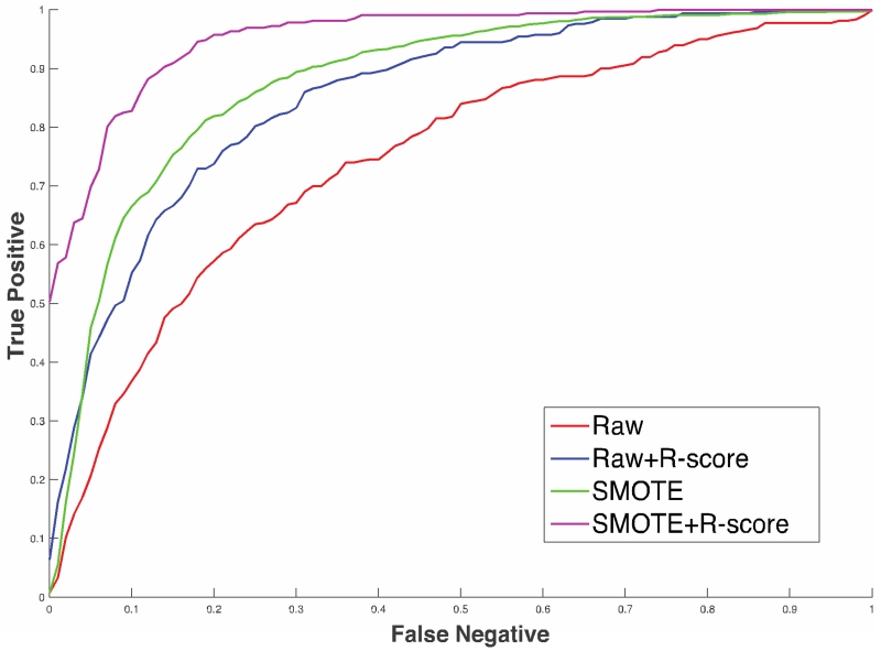
Figure 3 shows the result of a preliminary analysis of the data to compare the differences between raw data, r-scored data, resampled SMOTE data, and a combination of r-scored and resampled SMOTE data. Over internal 4-fold cross-validation, a combination of SMOTE and r-scored data produces the best results.

Figure 3.

Comparison of prognostic models with raw data, r-scored data and SMOTE

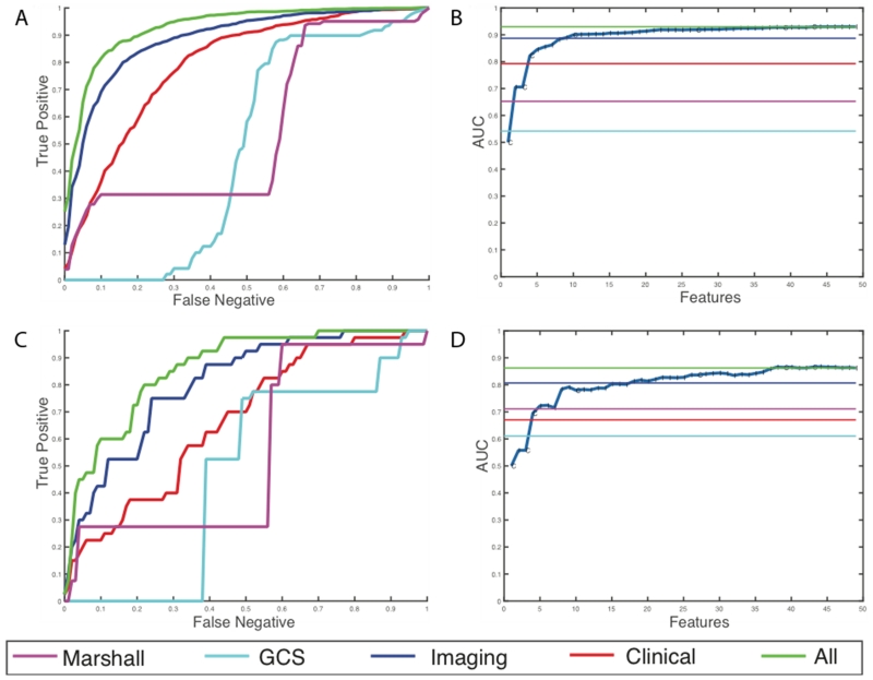
For discharge disposition, 61 of the initial 168 features were selected as the most stable features through mutual information selection. 49 of these 61 features are selected as a result of greedy forward selection. 7 of these features are clinical measures such as pulse, BP, hematocrit, arrival condition, injury severity score, and admission GCS scores and the rest are imaging features. We stop selection of features when at least three new features added to the model produce no statistically significant improvement. Table 3 and Figure 4 show the results of the analysis for the high-risk outcome of discharge disposition. We can see that latent image features obtained from the CTs are better predictors of mortality and quality of life (external AUC = 0.81) than all the clinical features together (external AUC = 0.67). Individual predictive performances of the Marshall CT class and the GCS scores at admission are shown. These scores have a very high false negative rate, which means that using these scores alone at admission misses a large percentage of high-risk cases. A prognostic model that combines the imaging features with the clinical features has the best predictive value of the discharge disposition, producing an external AUC of 0.86.

Table 3.

Discharge disposition results

Features	Average of 10-fold internal cross-validation				External holdout set
	Overall accuracy	Sensitivity	Specificity	AUC	Overall accuracy	Sensitivity	Specificity	AUC
Imaging + Clinical	86.2%	87.3%	85%	0.93	79.1%	80%	78%	0.86
Imaging only	81.9%	81.8%	82%	0.89	75.46%	75%	76%	0.81
Clinical only	72.95%	73.7%	72%	0.79	61.81%	62.5%	61%	0.67
Marshall	62.99%	86.1%	37%	0.65	62.94%	80%	43%	0.71
GCS	63.16%	77%	47%	0.54	63.9%	75%	51%	0.61

Figure 4.

Results for prediction of high-risk discharge disposition cases. (a) Average ROC curves internal cross-validated sets (b) Average effect of each new feature that is added via the greedy feature selection method (c) ROC curve for the holdout dataset (d) Effect of each new feature that is added via the greedy feature selection method in the holdout dataset.

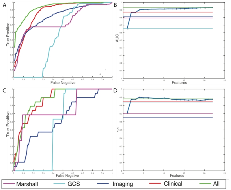
For the discharge GCS model, 22 of the initial 168 features were selected after elimination through mutual selection and greedy forward selection. 8 of these 22 features are clinical measures such as pulse, BP, respiration rate, arrival condition, injury severity score, and admission GCS scores. This model selects only 14 imaging features. Table 4 and Figure 5 show the results of the analysis for the high-risk outcome of discharge GCS scores. In this case, the clinical features are better predictors of functional outcomes than imaging features with an AUC of 0.85. However, addition of imaging features still improves the overall predictive power, by improving the AUC from 0.85 to 0.88 in the external hold out set. Moreover, we observe that the patterns of prediction in both internal cross validation is similar to prediction in external hold-out sets which provides assurance that the models are developed without over-fitting of the training data.

Table 4.

Discharge GCS results

Features	Average of 10-fold internal cross-validation				External holdout set
	Overall accuracy	Sensitivity	Specificity	AUC	Overall accuracy	Sensitivity	Specificity	AUC
Imaging + Clinical	82.45%	82.9%	82%	0.91	82%	89%	73%	0.88
Imaging only	72.57%	72.2%	73%	0.81	60.82%	68.5%	51%	0.65
Clinical only	78.2%	77.5%	79%	0.84	81.1%	82%	73.6%	0.85
Marshall	65.8%	93.7%	31%	0.79	71.9%	100%	36%	0.85
GCS	68.0%	89.16%	41%	0.56	74.6%	94.7%	50%	0.70

Figure 5.

Results for prediction of high-risk discharge GCS cases (a) Average ROC curves internal cross-validated sets (b) Average effect of each new feature that is added via the greedy feature selection method (c) ROC curve for the holdout dataset (d) Effect of each new feature that is added via the greedy feature selection method in the holdout dataset.

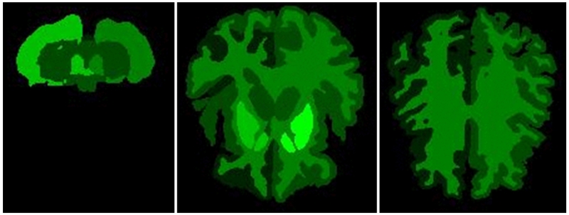
Figure 6 shows the regions of the brain from which the most features have been selected as predictive in the Discharge disposition model. Bright green indicates regions with the highest number of significant features selected in the greedy forward selection step. Black indicates zero features selected from the region.

Figure 6.

Axial sections of regions that have the highest number of predictive volume, intensity, and texture features.

4. DISCUSSION

Analysis of clinical and imaging data for outcome prediction in TBI is challenging because of data variability, lack of reliability, over-fitting, and unequal representation of multiple outcomes. The methods that we present in this paper overcome these problems. We used multi-atlas segmentation to calculate latent image features. The 4-fold feature selection and logistic regression approach shows strong evidence that adding imaging information to standard clinical scores improves the prognostic model. We observe that traditional diagnostic scores used in the ED, such as the Marshall CT classification and the GCS score, have a high false negative rate when used alone, and need to be examined in the context of other clinical and imaging features. Even though one would expect a correlation between functional outcomes based on GCS score and discharge disposition, we observe that they have very different manifestations. Clinical features are more important predictors of the discharge GCS whereas image features are important for the later.

In fact, discharge GCS model, which is an assessment based on mostly clinical measures misses some of the cases, which resulted in death or transfer to hospice. In 15 of the 40 cases labeled as “high-risk” in the discharge disposition hold-out dataset, the subject had a very high last recorded GCS (>13) but died in the hospital (4) or was admitted to a hospice/extended care facility (11). Our discharge disposition model, which selected strong imaging features, successfully identified 10 of these 15 cases, including 3 of 4 deaths, even though the clinical markers for these patients indicated good health. This further validates our assertion that the addition of imaging features greatly improves prognostic value by adding latent information in images to the predictive models.

References

- [1].Marshall LF, Marshall SB, Klauber MR, et al. A new classification of head injury based on computerized tomography. Special Supplements. 1991;75(1S):S14–S20. [Google Scholar]
- [2].Ratanalert S, Chompikul J, Hirunpat S, et al. Prognosis of severe head injury: an experience in Thailand. Br J Neurosurg. 2002;16(5):487–93. doi: 10.1080/0268869021000030311. [DOI] [PubMed] [Google Scholar]
- [3].Walker WC, Ketchum JM, Marwitz JH, et al. A multicentre study on the clinical utility of post-traumatic amnesia duration in predicting global outcome after moderate-severe traumatic brain injury. J Neurol Neurosurg Psychiatry. 2010;81(1):87–9. doi: 10.1136/jnnp.2008.161570. [DOI] [PubMed] [Google Scholar]
- [4].Cremer OL, Moons KG, van Dijk GW, et al. Prognosis following severe head injury: Development and validation of a model for prediction of death, disability, and functional recovery. Journal of Trauma and Acute Care Surgery. 2006;61(6):1484–1491. doi: 10.1097/01.ta.0000195981.63776.ba. [DOI] [PubMed] [Google Scholar]
- [5].Plassard AJ, Kelly PD, Asman AJ, et al. Revealing Latent Value of Clinically Acquired CTs of Traumatic Brain Injury Through Multi-Atlas Segmentation in a Retrospective Study of 1,003 with External Cross-Validation. Proc SPIE Int Soc Opt Eng. 2015:9413. doi: 10.1117/12.2081329. [DOI] [PMC free article] [PubMed] [Google Scholar]
- [6].Chawla NV, Bowyer KW, Hall LO, et al. SMOTE: synthetic minority over-sampling technique. Journal of artificial intelligence research. 2002:321–357. [Google Scholar]
- [7].Asman AJ, Landman BA. Hierarchical performance estimation in the statistical label fusion framework. Medical image analysis. 2014;18(7):1070–1081. doi: 10.1016/j.media.2014.06.005. [DOI] [PMC free article] [PubMed] [Google Scholar]