Whole Abdominal Wall Segmentation using Augmented Active Shape Models (AASM) with Multi-Atlas Label Fusion and Level Set

Abstract

The abdominal wall is an important structure differentiating subcutaneous and visceral compartments and intimately involved with maintaining abdominal structure. Segmentation of the whole abdominal wall on routinely acquired computed tomography (CT) scans remains challenging due to variations and complexities of the wall and surrounding tissues. In this study, we propose a slice-wise augmented active shape model (AASM) approach to robustly segment both the outer and inner surfaces of the abdominal wall. Multi-atlas label fusion (MALF) and level set (LS) techniques are integrated into the traditional ASM framework. The AASM approach globally optimizes the landmark updates in the presence of complicated underlying local anatomical contexts. The proposed approach was validated on 184 axial slices of 20 CT scans. The Hausdorff distance against the manual segmentation was significantly reduced using proposed approach compared to that using ASM, MALF, and LS individually. Our segmentation of the whole abdominal wall enables the subcutaneous and visceral fat measurement, with high correlation to the measurement derived from manual segmentation. This study presents the first generic algorithm that combines ASM, MALF, and LS, and demonstrates practical application for automatically capturing visceral and subcutaneous fat volumes.

1. INTRODUCTION

The human abdominal wall is an important structure protecting organs within the abdominal cavity. Moreover, there is increasing clinical interest the quantification of subcutaneous and visceral fat classified as fat tissue outside and inside the abdominal wall, respectively [1]. Ratios between these two fat tissues enable the prospective and retrospective analyses of various clinical conditions including ventral hernias, cardiovascular diseases, laboratory markers of metabolic syndrome, and cancers. Hence, segmentation of the abdominal wall is an important image analysis problem.

Computed tomography (CT) scans are routinely acquired for the diagnosis and prognosis of abdomen-related disease. To date, there are no available automated tools for whole abdominal wall segmentation on clinically acquired CT. Major challenges include (1) variations across subjects, (2) variations across axial slices along the cranial-caudal direction, and (3) complexity in shape and appearance of the wall itself and surrounding tissues (Figure 1). In a previous study, we characterized the whole abdominal wall structure as enclosed by the outer and inner surface, bounded by the xiphoid process (XP) and pubic symphysis (PS) [2]. Manually tracing the abdominal wall structures is time-consuming; it takes over an hour per scan to label sparsely on axial slices every 5 cm [2]. Ding et al. [3] built Gaussian mixture models for the intensity profiles of abdominal muscles after identifying skin and bones, used the extracted features to deform a surface mesh and register to the inner wall over the region with the presence of rib cage. Zhu et al. [4] developed an interactive tool to delineate the inner wall on a few slices, and propagate the surface to the entire abdomen using 3D B-spline interpolation. These were developed as tools to remove the abdominal wall to improve the registrations and visualization of the internal organs. Yao et al. [5] separated the subcutaneous and visceral fat by a single surface at the abdominal wall driving by active contour models (ACM). Zhang et al. [6] presented an atlas-based approach to segment the thoracic, abdominal, and pelvic musculature using five pre-defined muscle atlas models, and then refined with ACM. Xu et al. [7] used texture features to improve the level set segmentation of the outer abdominal wall on hernia patients. So far, none of these methods addressed the whole abdominal wall segmentation.

Figure 1.

For each patient (A and B), one coronal slice and five axial slices at different locations are shown to illustrate variability in anatomy and wall appearance.

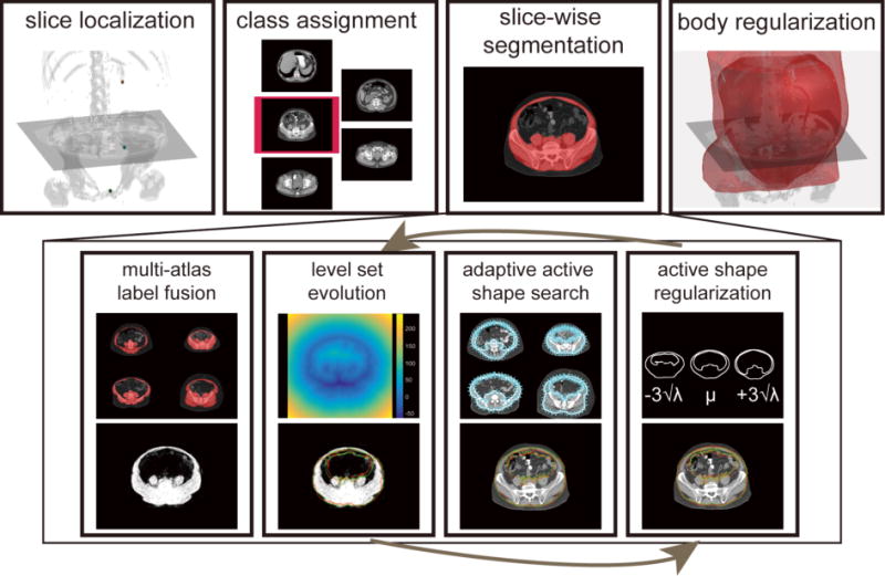
Herein, we proposed an automatic approach that combines the merits of active shape model (ASM [8]), multi-atlas label fusion (MALF [9, 10]), and level set (LS [11]) to provide robust segmentation of the whole abdominal wall in a slice-wise manner (Figure 2). We call this approach an augmented active shape model (AASM). Briefly, the central framework builds on ASM; where each landmark, under the shape constraint, is updated based on the pre-trained models of the local intensity profiles along its normal directions. MALF provided a probabilistic estimation regardless of the complex underlying structures by transferring a set of canonical atlases to the target space via image registrations, based on which a region-based LS using Chan-Vese (CV) algorithm [12] drives the landmark updates on a global sense. The augmentation with MALF and LS effectively extends the searching range, and enhances the robustness of ASM. On top of the slice-wise segmentation, we localize three biomarkers, i.e., XP, PS, and umbilicus (UB) for each target volume using random forests. Based on their locations, we assigned each axial slice between XP and PS to one of five classes, where each class was trained individually with exclusive atlases. Finally, the slice-wise segmentations were regularized across the body via Gaussian smoothing. The segmentation of the whole abdominal wall and the subcutaneous and visceral fat measurements were validated on 184 axial slices manually labeled on 20 scans.

Figure 2.

Flowchart of the proposed AASM approach for whole abdominal wall segmentation. For a target volume, XP, SP, and UB are localized by random forest, based on which, each axial slice between XP and SP is extracted and assigned to one of five classes. The slice-wise segmentation uses region-based LS to evolve on the probabilistic estimation obtained by MALF to augment the traditional active shape search by global optimization. The active shape regularization preserves the abdominal wall topology. Note the red and green markers at the bottom row indicate the landmark positions before and after the operation of the associated block. Body regularization is achieved by 3D Gaussian smoothing the collected slice-wise segmentation.

2. THEORY

In this section, we focus on the development of ASM augmentation. Implementation details can be found in the Methods and Results section.

Active shape model construction

Consider in each of s training images and a structure characterized by n landmarks. The landmark coordinates (x₁, y₁),…(x_n, y_n) are collected in a shape vector for each training set as x = (x₁,y₁, …, x_n, y_n)^T. The mean $\overline{\mathbf{x}}$, and covariance S of the shape vectors are computed, where

$$\overline{x}=\frac{1}{s}{\displaystyle \sum _{i=1}^s{x}_i,}S=\frac{1}{s-1}{\displaystyle \sum _{i=1}^s\left(x_i-\overline{x}\right){\left(x_i-\overline{x}\right)}^T.}$$ (1)

Using principle component analysis (PCA), the Eigenvectors p_i with its associated Eignenvalues λ_i are collected. Typically, Eigenvectors correspondent to the t largest Eigenvalues were retained to keep a proportion f_v of the total variance such that ${\sum }_{i=1}^t{\lambda }_i\ge f_v{\sum }_t{\lambda }_i$, where $\mathbf{P}=({\mathbf{p}}_1|{\mathbf{p}}_2|\dots |{\mathbf{p}}_t)$. Within this Eigensystem, any set of landmarks can be approximated by

$$x\approx \overline{x}+Pb$$ (2)

where b is a t dimensional vector given by

$$b=P^T\left(x-\overline{x}\right)$$ (3)

b can be considered as shape model parameters, and its values are usually constrained within the range of $\pm m_b\sqrt{{\lambda }_i}$ when fitting the model to a set of landmarks so that the fitted shape is regularized by the model.

Local appearance model and active shape search

The intensity profiles along the normal directions of each landmark are collected to build a local appearance model to suggest the locations of landmark updates when fitting the model to an image structure. For each landmark in the i^th training image, a profile of 2k + 1 pixels is sampled with k samples on each side of the landmark. Following [13], the profile is collected as the first derivative of the intensity, and normalized by the sum of absolute values along the profile, indicated as g_i. Assuming multivariate Gaussian distribution of the profiles among all training data, a statistical model is built for each landmark,

$$f\left(\mathbf{g}\right)=\left(\mathbf{g}-\overline{g}\right)S_g^{-1}\left(\mathbf{g}-\overline{g}\right)$$ (4)

where $\overline{\mathbf{g}}$ and S_g represent the mean and covariance, respectively. This is also called the Mahalanobis distance that measures the fitness of a newly sampled profile g to the model. Given a search range of m pixels (m > k) on each side of the landmark along the normal direction, the best match is considered with the minimum f(g) value among 2(m−k)+1 possible positions.

Level set evolution with Chan-Vese algorithm

In the level set context, the evolving surface is represented as the zero level set of a higher dimensional function ϕ(x, t), and propagates implicitly through its temporal evolution $\frac{\partial \varphi }{\partial t}$ with a time step dt. ϕ(x, t) is defined as signed distance function (SDF), with negative/positive values inside/outside the evolving surface, respectively. The CV algorithm evolves the SDF by minimizing the variances of the underlying image u₀ both inside and outside the evolving surface.

Given C₁=average(u₀) in {ϕ ≥ 0}, and C₂ = average (u₀) in {ϕ < 0}, the temporal evolution of CV can be written as

$$\frac{\partial \varphi }{\partial t}=\alpha \delta \left(\varphi \right)[\mu \kappa -{\left(u_0-C_1\right)}^2+{\left(u_0-C_2\right)}^2]$$ (5)

where δ (·) is the Dirac delta function, $\kappa =\text{div}\frac{\nabla \varphi }{\left|\mathit{\nabla }\varphi \right|}$ represents the curvature of SDF, α and μ are considered as the evolution coefficient and smoothness factor, respectively.

Adaptive active shape search

Let (x, y) be the current landmark position, ϕ₀ the current zero level set. Within each iteration of the active shape search, through j iterations of CV evolution, the zero level set moves to ϕ′₀. The zero-crossing point along the normal direction of (x, y) on ϕ′₀ is collected as (x′, y′), and considered as the new landmark position after LS evolution. Along (x′, y′), the gradient intensity profiles are sampled, then the active shape search suggest an updated position at (x″, y″) with its correspondent profile ${\mathbf{g}}^{″}=\underset{\mathbf{g}}{\mathrm{argmin}}f(\mathbf{g})$. The adaptively searched positions for all landmarks are then projected to the model space by Eq. 3. The shape is then regularized in Eq. 2 after the constraint on the model parameter.

3. METHODS AND RESULTS

Data

Under institutional review board supervision, abdominal CT data on 250 cancer patients that were acquired clinically were retrieved in anonymous form. 40 patients were randomly selected, where we used 20 as training datasets, and the other 20 for testing purposes. The field of views of the selected 40 scans range from 335 × 335 × 390 mm³ to 500 × 500 × 708 mm³, with various resolutions (0.98 × 0.98 × 5 mm³ ~ 0.65 × 0.65 × 2.5 mm³). Various numbers (78 ~ 236) of axial slices with same in-plane dimension (512 × 512) were found. All 40 scans were labeled using the Medical Image Processing And Visualization (MIPAV [14]) software by an experienced undergraduate based on our previously published labeling protocol [2], where essential biomarkers (XP, PS, UB) were identified, and the abdominal walls were delineated on axial slices spaced every 5 cm with some amendments (contour closure required here). 177 and 184 axial slices were obtained with whole abdominal wall labeled for the training and testing datasets, respectively.

Slice localization and class assignment

The proposed slice-wise segmentation was trained and tested on five exclusive classes given the position of the axial slices with respect to XP, PS, and UB. These three biomarkers were acquired from manual labeling for the training sets, while estimated using random forest for the testing sets. We used 10 random scans from the training data to characterize the centroid coordinates of the biomarkers with long-range feature boxes following [15], and yielded the estimated biomarkers positions on the testing data with a mean distance error of 14.43 mm. Four bounding positions were empirically defined among the vertical position of the three biomarkers to evenly distribute the available training data (25, 35, 50, 31, 36 slices for each class, ordered from bottom to top). Given a target testing volume, each axial slice between the estimated positions of XP and PS was extracted, and assigned a class based on the estimated bounding positions.

Slice-wise pre-processing

All slices (training and testing) were centered in the image after body extraction and background removal to reduce variations. A body mask can be obtained by separating the background with k-means clustering, and then filling holes in the largest remaining connected component. A margin of 50 pixels was padded to each side of the slices, which makes the slice size 612 × 612.

Multi-atlas label fusion

For each test slice, all training slices from the same class were considered as atlases, and non-rigidly registered to it using NiftyReg [16]. The registered atlases were combined by joint label fusion [10] to yield an probabilistic estimation of the abdominal wall. Default parameters were used for both registrations and label fusion.

Active shape model

On each training slice, landmarks were collected along the outer and inner wall contours using marching squares. The horizontal and vertical middle lines of the slice were used to divide each closed contour into four consistent segments across all slices assuming all patients were facing toward the same direction in the scan. 53 correspondent landmarks were then acquired on each of the segments via linear interpolation (212 for each of outer and inner wall). Each set of the landmarks was first centered to the origin, and then sets of landmarks from the same class were used to construct one active shape model covering 98% of the total variances. The shape updates were regularized within ± 3 standard derivations of the Eigenvalues.

Active shape search

An intensity gradient profile of 5 pixels was collected along each side the normal directions of each landmark (11 pixels in total) for training the local appearance model. The searching range during testing for the landmark update was 8 pixels along each side of the normal direction. A multi-level scheme (for both training and testing) was used to extend the searching range. We allowed 100 iterations for three levels of shape updates.

Level set evolution

A region-based LS evolution with five iterations using CV algorithm was used to drive the landmark movement based on the global probabilistic estimation within each iteration of the active shape search. The time step, evolution coefficient, and smoothness factor and was set to 0.01, 100000, and 0.1, respectively.

Customized configuration

In this study, a two-phase scheme was used to improve the robustness of whole abdominal wall segmentation. The proposed approach was first applied to only the outer wall. Initialized by the position of the outer wall segmentation, our approach was then applied to the combination of the outer and inner wall, while the outer wall landmark positions were fixed during the second phase shape updates. Active shape model and local appearance model were thus trained on (1) outer wall, and (2) outer and inner wall. The level set evolution for the second phase only considered the region within the outer wall segmentation obtained in the first phase.

Body regularization

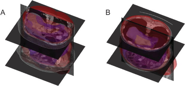
The slice-wise segmentations were transferred back to the original body space, converted into SDF, smoothed by a Gaussian 21 × 21 × 21 kernel with a standard deviation of 5, and finally converted to the binary segmentation of the whole abdominal wall for the body (Figure 3).

Figure 3.

Surface rendering of the segmented whole abdominal wall (red – outer surface, blue – inner surface) for two patients. Patients A and B correspond to those shown in Figure 1.

Fat Measurement

Following [5], the fat tissue was obtained by using a two-stage fuzzy-c means. For each slice, the subcutaneous fat was considered as outside the outer surface of the abdominal wall, while the visceral fat as inside the inner surface.

Results validation

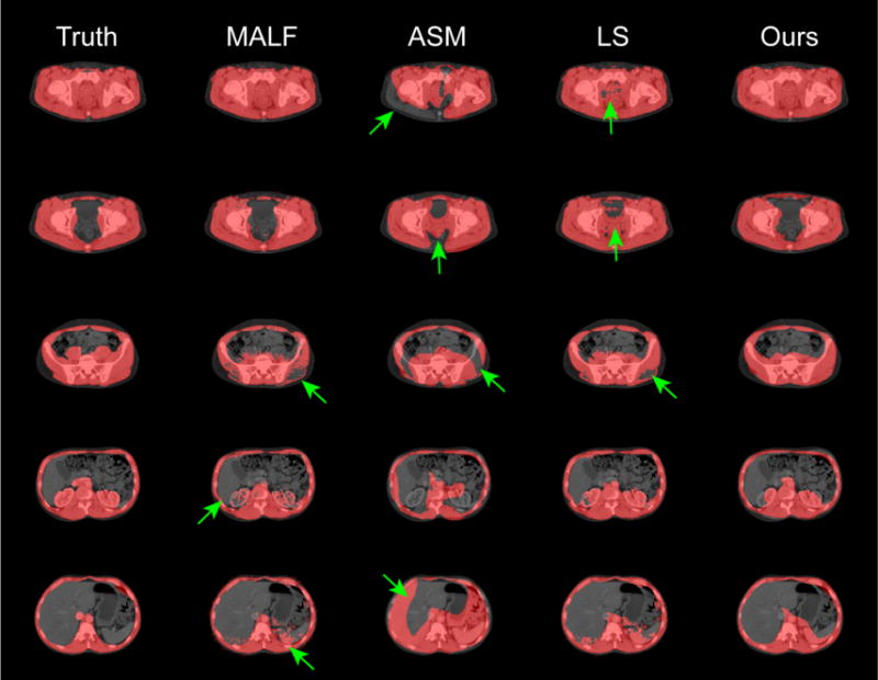
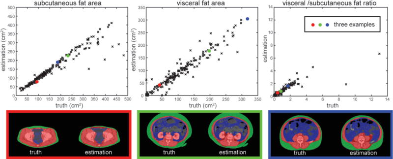
The segmentation results were validated against the manual labels on 184 testing slices using Dice similarity coefficient (DSC) and Hausdorff distance (HD) with comparison to results using MALF, ASM, and LS individually. Qualitatively, our proposed method presented the most robust result, while MALF and LS have speckles and holes in the segmentations, or leak into the abdominal cavity where structures with similar intensities to muscles were present. ASM was sensitive to initialization, and could be trapped into local minimum (Figure 4). Large decreases in HD were observed when using the proposed AASM approach without undermining the DSC performance. More importantly, the nature of ASM kept the topology of the abdominal wall, and enabled the compartmental fat measurement. The absolute differences in subcutaneous and visceral measure using our augmented ASM against the measurement using manual labels were largely reduced comparing to traditional ASM (Table 1). The Pearson’s correlation coefficient between our measurement and the truth was 0.93, 0.96, and 0.87 for subcutaneous fat, visceral fat, and the ratio of visceral to subcutaneous fat, respectively (Figure 5).

Figure 4.

Qualitative comparison of the proposed approach and other segmentation techniques applied individually. The green arrows indicate segmentation outliers including speckles, holes, over-segmentation, and label leaking problems

Table 1.

Quantitative comparison of the proposed AASM approach and other techniques applied individually.

Method	MALF	ASM	LS	AASM
DSC	0.89 ± 0.07	0.76 ± 0.14	0.89 ± 0.07	0.86 ± 0.09
HD (mm)	46.03 ± 14.45	47.74 ± 16.26	43.40 ± 15.34	33.80 ± 15.13
Abs. Diff. of S. Fat (cm2)	N/A	39.80 ± 52.32	N/A	16.72 ± 37.69
Abs. Diff. of V. Fat (cm2)	N/A	49.13 ± 48.14	N/A	15.38 ± 17.39

Note the subcutaneous fat area across the validated axial slices is 166.87 ± 108.01 cm², the visceral fat area is 105.12 ± 76.01 cm². Label fusion (LF), and level set (LS) cannot guarantee two closed surfaces for the outer and inner abdominal wall respectively, thus not applicable for fat area calculation.

Figure 5.

Validation of the fat measurement. The subcutaneous and visceral fat area, and the ratio of visceral to subcutaneous fat were measured based on the automatically segmented (estimation) and manually labeled (truth) abdominal wall. Three examples were illustrated where the red, blue, and green represent the segmented abdominal wall, visceral fat, and subcutaneous fat, respectively.

4. DISCUSSION

The abdominal wall and its surrounding structures are extremely complicated. Our definition of the whole abdominal wall covers thoracic, abdominal, and pelvic regions, and includes not only the musculature, but also the kidneys, aorta, inferior vena cava, lungs, and some related bony structures to make the inner and outer boundaries anatomically reasonable. In this study, we presented the first automatic AASM approach to coherently integrate three distinctive image segmentation techniques, i.e., ASM, MALF, and LS, and used it to segment the whole abdominal wall on CT scans. This challenging problem benefitted from the shape regularization and topology preservation of ASM, contextual robustness of MALF, and global optimization of region-based LS, and was thus handled appropriately by largely reducing HD comparing to methods using only individual techniques above. The whole abdominal wall segmentation also enabled the calculation of subcutaneous and visceral fat with a high correlation to its counterparts based on manual segmentation. Further improvement can be achieved by augmenting the training datasets, especially a better classification system for axial slices over various locations.

References

- 1.Summers RM, Liu J, Sussman DL, et al. Association between visceral adiposity and colorectal polyps on CT colonography. AJR American journal of roentgenology. 2012;199(1):48. doi: 10.2214/AJR.11.7842. [DOI] [PMC free article] [PubMed] [Google Scholar]
- 2.Allen WM, Xu Z, Asman AJ, et al. Quantitative anatomical labeling of the anterior abdominal wall. SPIE Medical Imaging. 2013 doi: 10.1117/12.2007071. 867312-867312-7. [DOI] [PMC free article] [PubMed] [Google Scholar]
- 3.Ding F, Leow WK, Venkatesh S. Removal of abdominal wall for 3D visualization and segmentation of organs in CT volume. Image Processing (ICIP), 2009 16th IEEE International Conference on. 2009:3377–3380. [Google Scholar]
- 4.Zhu W, Nicolau S, Soler L, et al. Fast segmentation of abdominal wall: Application to sliding effect removal for non-rigid registration. Abdominal Imaging. Computational and Clinical Applications. 2012:198–207. [Google Scholar]
- 5.Yao J, Sussman DL, Summers RM. Fully automated adipose tissue measurement on abdominal CT. SPIE Medical Imaging. 2011 79651Z-79651Z-6. [Google Scholar]
- 6.Zhang W, Liu J, Yao J, et al. Segmenting the thoracic, abdominal and pelvic musculature on CT scans combining atlas-based model and active contour model. SPIE Medical Imaging. 2013 867008-867008-6. [Google Scholar]
- 7.Xu Z, Allen WM, Baucom RB, et al. Texture analysis improves level set segmentation of the anterior abdominal wall. Medical physics. 2013;40(12):121901. doi: 10.1118/1.4828791. [DOI] [PMC free article] [PubMed] [Google Scholar]
- 8.Cootes TF, Taylor CJ, Cooper DH, et al. Active shape models-their training and application. Computer vision and image understanding. 1995;61(1):38–59. [Google Scholar]
- 9.Rohlfing T, Brandt R, Menzel R, et al. Evaluation of atlas selection strategies for atlas-based image segmentation with application to confocal microscopy images of bee brains. NeuroImage. 2004;21(4):1428–1442. doi: 10.1016/j.neuroimage.2003.11.010. [DOI] [PubMed] [Google Scholar]
- 10.Wang H, Suh JW, Das SR, et al. Multi-atlas segmentation with joint label fusion. Pattern Analysis and Machine Intelligence, IEEE Transactions on. 2013;35(3):611–623. doi: 10.1109/TPAMI.2012.143. [DOI] [PMC free article] [PubMed] [Google Scholar]
- 11.Sethian JA. Level set methods and fast marching methods: evolving interfaces in computational geometry, fluid mechanics, computer vision, and materials science. Cambridge university press; 1999. [Google Scholar]
- 12.Chan TF, Vese L. Active contours without edges. Image Processing, IEEE Transactions on. 2001;10(2):266–277. doi: 10.1109/83.902291. [DOI] [PubMed] [Google Scholar]
- 13.Cootes T, Baldock E, Graham J. An introduction to active shape models. Image processing and analysis. 2000:223–248. [Google Scholar]
- 14.McAuliffe MJ, Lalonde FM, McGarry D, et al. Medical image processing, analysis and visualization in clinical research. Computer-Based Medical Systems, 2001. CBMS 2001. Proceedings. 14th IEEE Symposium on. 2001:381–386. [Google Scholar]
- 15.Criminisi A, Robertson D, Konukoglu E, et al. Regression forests for efficient anatomy detection and localization in computed tomography scans. Medical image analysis. 2013;17(8):1293–1303. doi: 10.1016/j.media.2013.01.001. [DOI] [PubMed] [Google Scholar]
- 16.Modat M, Ridgway GR, Taylor ZA, et al. Fast free-form deformation using graphics processing units. Computer methods and programs in biomedicine. 2010;98(3):278–284. doi: 10.1016/j.cmpb.2009.09.002. [DOI] [PubMed] [Google Scholar]