Identifying Cancer Biomarkers From Microarray Data Using Feature Selection and Semisupervised Learning

Abstract

Microarrays have now gone from obscurity to being almost ubiquitous in biological research. At the same time, the statistical methodology for microarray analysis has progressed from simple visual assessments of results to novel algorithms for analyzing changes in expression profiles. In a micro-RNA (miRNA) or gene-expression profiling experiment, the expression levels of thousands of genes/miRNAs are simultaneously monitored to study the effects of certain treatments, diseases, and developmental stages on their expressions. Microarray-based gene expression profiling can be used to identify genes, whose expressions are changed in response to pathogens or other organisms by comparing gene expression in infected to that in uninfected cells or tissues. Recent studies have revealed that patterns of altered microarray expression profiles in cancer can serve as molecular biomarkers for tumor diagnosis, prognosis of disease-specific outcomes, and prediction of therapeutic responses. Microarray data sets containing expression profiles of a number of miRNAs or genes are used to identify biomarkers, which have dysregulation in normal and malignant tissues. However, small sample size remains a bottleneck to design successful classification methods. On the other hand, adequate number of microarray data that do not have clinical knowledge can be employed as additional source of information. In this paper, a combination of kernelized fuzzy rough set (KFRS) and semisupervised support vector machine (S³VM) is proposed for predicting cancer biomarkers from one miRNA and three gene expression data sets. Biomarkers are discovered employing three feature selection methods, including KFRS. The effectiveness of the proposed KFRS and S³VM combination on the microarray data sets is demonstrated, and the cancer biomarkers identified from miRNA data are reported. Furthermore, biological significance tests are conducted for miRNA cancer biomarkers.

The development of simple data mining tests for early cancer detection is one of the top priorities in cancer research. This article proposes a combination of kernelized fuzzy rough set (KFRS) and semisupervised support vector machine (S³VM) for predicting cancer biomarkers from one miRNA and three gene expression datasets. Biomarkers are discovered employing three feature selection methods including KFRS. The effectiveness of the proposed KFRS and S³VM combination on the microarray datasets is demonstrated, and the cancer biomarkers identified from miRNA data are reported. Furthermore, biological significance tests are conducted for miRNA cancer biomarkers.

I. Introduction

Developing simple data mining tests that allow early cancer detection is one of the top priorities in cancer research field. Such tests will impact patient care and outcome through disease screening and early detection. Large number of gene expression/miRNA data and their diverse expression patterns indicate that they are likely to be involved in a broad spectrum of human diseases. For example, the miRNAs found based on the combinations of computational and experimental techniques [1] can be potentially used to study their involvement in different diseases. It has been found in several studies that some miRNAs are differentially expressed in normal and cancerous tissues. This finding suggests possible links between miRNAs and oncogenesis [2]. Furthermore, some miRNAs are differentially expressed in tissue-specific tumors, which indicate that it might be possible to diagnose the cancer type from these onco-miRNA signatures. Hence the development of suitable machine learning techniques for finding onco-miRNAs that target onco-genes is an important task that could provide alternate ways of diagnosis and therapy of the diseases.

Microarray data analysis methods can be broadly grouped into unsupervised, supervised and semisupervised methods. Unsupervised analysis or class discovery is an unbiased analysis of microarray data. No prior class information is used and clustering methods are employed to group the samples. Extensive studies for gene expression analysis lead to different methodological techniques including gene clustering and gene marker identification [3]–[8]. A wide variety of clustering techniques in the field of computational biology, bioinformatics, soft computing and geoscience can be found in [9]–[11].

In the case of supervised analysis, previous knowledge is taken into account. Often tumor samples for microarray studies come from well-defined groups, for example good and poor prognosis patients. The aim is then to identify genes or develop a model that is able to assign patients to the good or poor prognosis class based on the microarray data, of its corresponding tumor. A few examples of modeling strategies are naive Bayesian (NB) classifiers [12]–[14] decision trees [15], support vector machines [16], [17] and -nearest neighbor (KNN) classifiers [18], [19].

On the other hand, semisupervised methods are also being used for gene classification by jointly employing both labeled and unlabeled data [20]. Microarray data are being exploited for semisupervised gene expression analysis leading to a better understanding of genetic signatures in cancers and improve treatment strategies including peptide identification in shotgun proteomics [21], protein classification [22], prediction of transcription factor-gene interaction [23] and gene expression based cancer subtypes discovery [24]–[29]. A microarray dataset is two dimensional matrix , consisting of samples and biomolecules. Each element represents the expression level of the th microarray for th sample. To identify biomarkers for semisupervised classification, the problem is modeled as a feature selection problem where the genes or miRNAs are considered as features.

Selection of informative genes [30] is an important part for the analysis of microarray data. Successful feature selection has several advantages in such situations where thousands of features are involved. First, dimension reduction is employed to reduce the computational cost. Second, reduction of noises is performed to improve classification accuracy. Finally, extraction of more interpretable features or characteristics that can be helpful to identify and monitor the target diseases.

In this work, we have investigated several feature selection methods namely kernelized fuzzy rough set (KFRS) [31], [32], fuzzy preference based rough set (FPRS) [33] and consistency based feature selection (CBFS) [34]. Subsequently, different tumor types are predicted based on these selected microarray biomarkers using our recently proposed transductive (semisupervised) SVM (TSVM) [24] and compared with the performances of the traditional supervised methods including SVM [35], KNN [36] and naive Bayesian classifiers [37]. The proposed method (KFRS + TSVM) outperforms (CBFS +TSVM) [24], (FPRS + TSVM) [25] as well as KNN and naive Bayes classifiers in combination with these feature selection techniques on the four publicly available microarray datasets (i.e., three gene-expression and one miRNA datasets). Experimental results of the proposed method have proved to be effective based on the comparative study conducted on these microarray datasets. Furthermore, we have investigated how the selected miRNAs are associated with different types of cancer.

The rest of the article is organized as follows: The next section briefly introduces ISVM/TSVM algorithms. Proposed technique is provided in section III. Section IV describes the datasets and preprocessing. Section V presents results and discussion followed by conclusion in section VI.

II. Basic Ideas of Inductive and Transductive SVM

A. Inductive SVM

Inductive SVM (ISVM) is a general class of learning architecture originated in modern statistical learning theory [35]. Given a training dataset, the SVM training algorithm obtains the optimal separating hyperplane in terms of generalization error. In a binary classification problem, let be the set of training examples, where is the label associated with input pattern . In a learning problem, the task is to estimate a function from a given class of functions that correctly classifies unseen examples by computing the . In the case of pattern recognition, this means that given some new patterns , the classifier predicts the corresponding .

Following nonlinear transformation, the parameters of the decision function are determined by the following minimization problem:

subject to

where is a user-specified, positive, regularization parameter in Eqn. (1), The variable are the so called slack variables. The cost function in Eqn. (1) constitutes the structural risk, which balances empirical risk. The regularization parameter controls this trade off.

B. Transductive SVM

To alleviate the problem of small-size training set, transductive SVM was proposed in [35]. Compared to traditional SVM (also called inductive SVM), TSVM is often more promising and can provide better performance. TSVM seeks largest separation in presence of both labeled and unlabeled data through regularization. At the initial iteration, the standard SVM is used to obtain an initial discriminating hyperplane based on the labeled data alone. The trained SVM is then used to obtain the labels of the unlabeled samples. These are called semilabeled samples. Subsequently, useful transductive samples are selected from the semilabeled samples according to a given criterion. A hybrid training set is thus obtained consisting of the original labeled and transductive sets. The resulting hybrid training set is then used at the next iteration to find a more reliable separating hyperplane and the process is repeated. We describe the semisupervised SVM (S³VM) approach as follows.

Given a set of independent, identically distributed labeled examples and another set of unlabeled examples from the same distribution, the hyperplane separates both labeled and transductive samples with the maximal margin and is derived by minimizing:

subject to

In order to handle the nonseparable and transductive samples, similar to standard ISVMs, the slack variables and and associated penalty values and of both the labeled and transductive data objects are introduced. is the number of extracted semilabeled samples in the transductive process (. Like ISVM, training the TSVM corresponds to solving the above optimization problem.

Finally, the decision function of the TSVM after setting the Lagrange multipliers and is formulated as:

where the function is called the kernel function.

C. Kernel Functions

Using kernels, the optimal margin SVM classifier is turned into a high performance classifier by implicitly mapping the input vector into a high dimensional feature space. Some commonly used kernels to develop different SVM and other kernel based classifiers satisfying Mercer’s condition [38] are as follows.

• 1)
  Linear Kernel:

  
• 2)
  Polynomial kernel:

  
• 3)
  RBF kernel:

  
• 4)
  Sigmoid kernel:

  

  Eqn. (6) represents a linear kernel that computes a dot product in feature space. Eqn. (7) is a polynomial kernel where , is a constant that defines the kernel order. The RBF kernel is represented by Eqn. (8) where is the weight. On the other hand, Eqn. (9) shows a particular kind of two-layer sigmoid neural network which essentially serves as a similarity measure between and . It is to be noted that each kernel has a dot product term (. to measure the similarity between two vectors and . In this work, RBF kernel function has been utilized for mapping the input vectors. However, other kernel functions can be used to design SVM/TSVM.

III. Proposed Technique

The proposed method uses kernelized fuzzy rough set (KFRS) to find a set of biomarkers from the microarray datasets. Subsequently, the biomarkers are then used to distinguish to classes of samples using TSVM. To study the performance of the proposed method, we have used two well-known feature selection methods: fuzzy preference based rough set (FPRS) and consistency based feature selection (CBFS). Finally, computational and biological validations have been performed. Different feature selection methods and TSVM algorithm have been described as follows.

A. Kernelized Fuzzy Rough Set for Feature Selection

High level of similarity between kernel methods and rough sets can be obtained using kernel matrix as a relation [31]. Kernel matrices could serve as fuzzy relation matrices in fuzzy rough sets. Taking this into account, a bridge between rough sets and kernel methods with the relational matrices was formed [31]. Kernel functions are used to derive fuzzy relations for rough sets based data analysis. In this study, Gaussian kernel approximation has been used to construct a fuzzy rough set model, where sample spaces are granulated into fuzzy information granules in terms of fuzzy -equivalence relations computed with Gaussian kernel. The details on kernelized fuzzy rough set model is available in [31].

Formally, the forward greedy search algorithm based on Gaussian kernel approximation [32] can be written as:

Algorithm 1

• Input:Sample set , feature set , decision and stopping threshold
• Output::

  reduct

• Step 1:

  Initialize red to an empty set and to 0.

• Step 2:
  For each attribute , compute

  
• Step 3:

  Find the maximal and the corresponding attribute

• Step 4:
  Add attribute to if it satisfies

  
• Step 5:

  Assign to

• Step 6:

  Repeat steps 2–5 while

• Step 7:

  Return

Initially, the algorithm starts with an empty set of attribute. Subsequently, it evaluates the remaining attributes at each iteration and selects feature producing the maximal fuzzy dependency . Algorithm for the computation of dependency with Gaussian kernel is available in [32]. The algorithm terminates when adding any of the remaining attributes does not satisfy step 4 in the above algorithm. The output of the algorithm is a reduced feature set.

The fuzzy dependency can be computed as follows:

• Input:Sample set , feature set , decision and parameter
• Output:

  dependency of to

• Step 1:

  

• Step 2:

  to

• Step 3:

  find the nearest sample of with a different class

• Step 4:

  

• Step 5:

  return

The algorithm will remove those features from the data which would receive low dependency values.

B. Feature Selection Using Fuzzy Preference Based Rough Set

Given a universe of finite objects , a fuzzy preference relation is regarded as a fuzzy set on the product set , which is represented by a membership function : [0, 1]. If the cardinality of is finite, the fuzzy preference relation can be represented by an matrix where is the preference degree of over . If , it shows that and are equally preferable; indicates is preferred to , while means is absolutely preferred to . On the other hand, shows is preferable to . Here, the preference matrix is usually regarded to be an additive reciprocal, i.e., , In practice, preference structures are represented by a set of ordinal discrete or numerical values.

Given a universe of finite objects and is a nonempty finite set of attributes to characterize the objects. The feature value of is represented by where (for example, is a numerical feature. The upward and downward fuzzy preference relations over are formulated as:

and

where is a user defined positive constant.

The function , is the Logsig sigmoid transfer function used in neural networks. The forward greedy search algorithm based on fuzzy preference rough set is available in [33].

C. Consistency Based Feature Selection

Dash and Liu [34] introduced consistency function that attempts to maximize the class separability without deteriorating the distinguishing power of the original features. Consistency measure is computed using the properties of rough sets. Rough sets provide an effective tool which deals with the inconsistency and incomplete information. This measure attempts to find a minimum number of features that separate classes as consistently as the full set of features can. In classification, it is used to select a subset of original features which is relevant for increasing accuracy and performance, while reducing cost in data acquisition. When a classification problem is defined by features, the number of features can be very large, many of which are likely to be redundant. Therefore, a feature selection criterion is defined to select relevant features. Class separability constraint is usually employed as one of the basic selection criteria. Consistency measure can be used as a selection criterion that heavily depends on class information and aims to keep the discriminatory power of the actual features. This measure is defined by inconsistency rate and its method of computation can be found in [24] and [34].

D. Other Feature Selection Techniques

The objective of feature selection is to extract a subset of relevant features which is useful for model generation. Many mining algorithms don’t perform well with large number of features. These unwanted features need to be removed before any mining algorithm is applied. In the process of feature selection, the nature of training data is usually labeled, unlabeled or partially labeled leading to the development of supervised, unsupervised and semisupervised feature selection algorithms. Depending on how and when the utility of selected features is evaluated, different approaches are used in practice, which are broadly divided into three categories: filter, wrapper and embedded methods. For example, signal-to-noise-ratio (SNR) [39] uses filtering scheme to select relevant features. It is a correlation based feature ranking algorithm used in a forward selection way to rank features individually in terms of a correlation-based metric, and then top-ranked features are selected. Minimum-redundancy-maximum-relevance (mRMR) selects top-ranking features usually based on mutual information, correlation, or distance/similarity scores [40]. -score [41] is used for binary problem. -score [42] is used to test if a feature is able to well separate samples from different classes by considering between class variance and within class variance. Feature selection via chi-square test is another, very commonly used method [43]. This method evaluates the worth of a feature by computing the value of the chi-squared statistic with respect to the class label.

E. Classification by TSVM

In this study, we have applied the TSVM classifier proposed by Maulik et al. [24] on the selected gene and miRNA subsets obtained by the different feature selection methods. Training the TSVM algorithm can be roughly outlined as the following steps:

Step 1: Specify and and execute an initial learning using the original training set to obtain a trained SVM classifier.

Step 2: Compute the decision function values of all the unlabeled samples using the trained SVM classifier. Obtain label vector of the unlabeled set. Select all the positive and negative semilabeled (transductive) samples within the margin band and add them to the original training set to obtain a hybrid training set.

Step 3: Retrain the SVM classifier using this hybrid training set. Obtain the label vector of the unlabeled set. Select all the positive and negative semilabeled samples within the margin band.

Step 4: Select the common transductive samples between the previous and current transductive samples.

Step 5: Remove the previous transductive samples from the hybrid training set and add the resultant transductive set obtained from step 4.

Step 6: Repeat steps 3–5. The algorithm finishes after a finite number of iterations.

The algorithm is capable of reducing the misclassification rate of the transductive samples at each iteration through a process of successive filtering between the transductive sets which results in increased accuracy. The SVMs play the role to separate positive and negative samples, while the transductive inference successively searches more reliable discriminant function employing additional unlabeled samples. Intuitively, unlabeled patterns guide the linear boundary away from the dense regions. Fig. 1 shows the effect of the unlabeled patterns to determine maximum margin. Further details of the algorithm is available in [24].

FIGURE 1.

With labeled data only, the maximum margin is plotted with dotted lines. With both labeled and newly labeled data (small circles), the maximum margin boundary would be the one with solid lines.

IV. Datasets and Preprocessing

This section presents microarray datasets, semisupervised technique and model selection.

A. Microarray Datasets

In this paper, three gene microarray datasets publicly available at website [44] and one miRNA dataset are used. Since classification is a typical and fundamental issue in diagnostic and prognostic prediction of cancer, different combinations of methods are studied using the four datasets.

• 1)Small Round Blood Cell Tumors (SRBCT): The Small round blood cell tumors are four different childhood tumors named so because of their similar appearance on routine histology. The number of samples is 83 and total number of genes is 2308. They include Ewings sarcoma (EWS) (29 samples), neuroblastoma (NB) (18 samples), Burkitt’s lymphoma (BL) (11 samples) and rhabdomyosarcoma (RMS) (25 samples).
• 2)Diffuse Large B-Cell Lymphomas (DLBCL): Diffuse large B-cell lymphomas and follicular lymphomas are two B-cell lineage malignancies that have very different clinical presentations, natural histories and response to therapy. The dataset contains 77 samples and 7070 genes. The subtypes are diffuse large B-cell lymphomas (DLBCL) (58 samples) and follicular lymphoma (FL) (19 samples).
• 3)Leukemia: Leukemia is an affymetrix high-density oligonucleotide array that contains 5147 genes and 72 samples from two classes of leukemia: 47 acute lymphoblastic leukemia (ALL) and 25 acute myeloid leukemia (AML).
• 4)MicroRNA Dataset: We have downloaded a publicly available miRNA expression dataset from the web- site: http://www.broad.mit.edu/cancer/pub/miGCM/. The dataset contains 217 mammalian miRNAs from different cancer types. From this, we have selected six datasets consisting of the samples from colon, kidney, prostate, uterus, lung and breast. Each dataset is presented by all the 217 miRNAs [45]. Table 1 presents the normal and tumor sample counts of each of the tissue types. Each sample vector of the datasets is normalized to have mean 0 and variance 1. The resulting single dataset contains two classes of samples, one representing all the normal samples with 32 examples and another representing tumor samples having 43 examples. The dataset is first randomized and then partitioned into training (38 samples) and test set (37 unlabeled samples). While dividing into training and test sets, it is ensured that both training and test sets contain atleast one sample from normal and malignant samples of each of the tissue types. Feature selection algorithms are applied on the training set to extract informative miRNAs.

TABLE 1.

The number of normal and tumor samples present in each tissue type.

B. Semisupervised Classification

For the purpose of semisupervised classification, the training set is further sub-sampled with different rates to simulate ill-posed classification (i.e., the available labeled samples are often not representative enough of the test data distribution) problems. For example, using 38 training samples from miRNA data, training subsets of size 10, 15 and 20 are randomly selected resulting in atleast one sample (i.e., absence of a sample for each class would reject the iteration and resample the training set) for each class. For each size, ten different small training subsets are realized using a random procedure. The test set is used as unlabeled set. Accuracy assessment is carried out on the test set. However, these samples have not been considered for model selection. The same procedure is followed in case of gene expression datasets. Moreover, semisupervised classification is conducted using the training set (38 samples), while the same test set (37 samples) is used as unlabeled set (for miRNA data only).

C. Model Selection and SVM Training

Once the training samples are gathered (i.e., 50% samples from the labeled datasets), the next step is to optimize parameters and (model selection) of the radial basis function (RBF) using grid search. It is not known beforehand which and are the best for one problem [46]. The goal is to identify good (, so that the classifier can accurately predict unknown data. Therefore, a common way is to use cross-validation because it can prevent the overfitting problem [46]. A grid search on and is recommended using cross-validation [46]. In -fold cross validation, first, the available training dataset is divided randomly into equal-sized subsets. Second, for each model-parameter setting, the SVM classifier is trained -times; during each time one of the subsets is held out in turn while the remaining subsets are used to train the SVM. The trained classifier is then tested using the held-out subset, and its classification accuracy is recorded. At the end, the classification accuracies are averaged to obtain an estimate of the generalization error of the SVM classifier.

In usual practice, five, or ten-fold cross validation is adopted for the tuning of SVM parameters. Therefore, we have used five-fold () cross validation to optimize and . For the parameters to be tuned, we let each of them vary among the candidate set {0.1, 0.2, 0.4, 0.8, 1.6, 3.2, 6.4, 12.8} to form different parameter combinations. Each combination of parameter choices is evaluated using five-fold cross validation, and the parameters with the best cross validation accuracy are identified (i.e., model with smallest generalization error). Consequently, we fixed the optimal (, for SVM training with different training subsets made up of different samples and with different sizes for a particular dataset.

V. Results and Discussion

In this section, performances of the different methods are presented in terms of average overall accuracies (%) and standard deviations. To establish the effectiveness and robustness of the proposed method, statistical tests are conducted using -statistic [41] and Wilcoxon signed rank test [47]. Moreover, we have used Area Under ROC (AUC) curves [48], -measure [42] to study the performances of different approaches in case of miRNA data.

A. Statistical Significance Tests

To establish that (KFRS + TSVM) (i.e., feature selection followed by classification) is superior to the other methods, we have used statistical significance tests such as one tailed paired -test [41] and Wilcoxon signed rank test [47] at the 5% significance level. Here, only the -test is presented as follows.

The common population variance is estimated as:

where , are the sample variances and are sample sizes. For small samples we use the test statistic

where are sample means and

B. Input Parameters

Gaussian RBF kernel function of the form where is the weight, has been used to design ISVM/TSVM. Each biomarker is rescaled between {−1, +1} as recommended in [46] before use with the classifiers. The value of is set equal to . However, other weighting strategies may also be used. The value of is assigned to 10 or, 15 experimentally. For KNN classifier, the value of is set to 3.

C. Identification of Cancer Biomarkers

Using the different feature selection techniques, we have identified cancer biomarkers from the four microarray datasets including the miRNA data. For instance, top five miRNA biomarkers that are mostly responsible for distinguishing a tumor class from the normal one, are extracted from the training set by each of the feature selection methods. For the purpose of illustration, top five miRNA markers selected by KFRS method and their expression levels (Up or Down) in tumor cells are reported in Table 2. Fig. 2 depicts the expression levels of the training and test datasets for five miRNAs. The heatmaps, organized as gene versus sample matrix, illustrate that the selected miRNAs are very informative in discriminating the classes. The miRNAs are indicated on the right side of the images. It appears from the figure that for both training and test datasets, the selected miRNAs are differentially expressed in benign and malignant classes.

TABLE 2.

MicroRNA markers extracted by the KFRS method.

FIGURE 2.

The heatmaps of the expression levels of the top five miRNA biomarkers selected by the KFRS method. Each row represents an miRNA marker and each column corresponds to a sample. The miRNAs are rearranged in a way the similarity within class and dissimilarity between classes are easily recognized.

D. Classifier Performances

We have explored the performance of (KFRS + TSVM) combination with eleven other methods. The results are averaged over best ten runs of the classifier for ten different training subsets of a particular size. The experimental results produced by different methods in terms of overall average accuracies and standard deviations are reported in Table 3 for the microarray datasets. It can be observed from the table that (KFRS + TSVM) outperforms (CBFS + TSVM) [24], (FPRS + TSVM) [25] and other combinations. Best results are shown in bold face. Confidence levels for the observed differences in overall accuracies between the (KFRS + TSVM) and the corresponding method, according to a one-tailed paired -test are also provided in Table 3.

TABLE 3.

Overall accuracies and standard deviations averaged over 10 runs of the different training subsets made up of 10, 15 and 20 samples of the four microarray datasets. Superscripts indicate the confidence levels for the difference in accuracy between the proposed (KFRS + TSVM) and the corresponding combination of algorithms using -statistic: 1 is 99.5%, 2 is 99%, 3 is 97.5%, 4 is 95%, 5 is 90% and 6 is below 90%.

Experimental results are summarized in Table 4. The second column indicates the number of domains in which (KFRS + TSVM) is more accurate than the corresponding classifier, versus the number in which it is less. For example, (KFRS + TSVM) is found to be more accurate than (FPRS + TSVM) across 12 domains and less in zero. The third column reports the results for those domains where accuracy difference is significant at the 5% level according to the -statistic. For example, the proposed method is significantly more accurate than (FPRS + TSVM) in seven domains. The forth column shows the -levels on the 12 accuracy differences at the 5% level using Wilcoxon signed rank test, which results in high confidence of the proposed method. For instance, -level of (KFRS + TSVM) is 1 (row 4 and column 4 element in Table 4 compared to (FPRS + TSVM) indicating that the difference in accuracies provided by (KFRS + TSVM) is significant with respect to those provided by (KFRS + TSVM) to reject null hypothesis at the 5% level. Finally, the overall average accuracies of the different methods across all datasets are shown in the fifth column. Based on the average accuracy values on the microarray datasets, it appears that the proposed method is significantly better than the other methods.

TABLE 4.

Overall performances provided by 12 different methods. Column 4 indicates the different in accuracies between (KFRS + TSVM) and the corresponding method Using Wilcoxon signed rank Test : 1 for p-level <0.05 and 2 otherwise.

Moreover, for the purpose of illustration, Fig. 3 shows the boxplot representing the % accuracy over 10 runs of the six different methods. It is evident from the figure that the boxplot corresponding to (KFRS + TSVM) is situated at the upper side of the figure, which indicates that (KFRS + TSVM) results in higher accuracy scores than those produced by the other techniques.

FIGURE 3.

The boxplot showing the accuracies produced by the ISVM/TSVM algorithms over the best 10 runs for the different training subsets of size 20 of miRNA dataset.

Next, we have reported the performances of the ISVM/TSVM algorithms on the test set using the training set of size 38 of miRNA dataset in Table 5. The test set has been used as unlabeled set. From the table, it can be observed that (KFRS + TSVM) and (KFRS + ISVM) achieved 100.00% and 97.30% accuracies, respectively. This confirms that KFRS method offers statistically significant miRNA cancer markers providing high performance of the classifiers. However, it is interesting to observe the significant accuracy difference (8.12%) between (FPRS + TSVM) and (FPRS + ISVM). Furthermore, ROC curves in Fig. 4 illustrate the performance of the six different methods. From the figure, it can be seen that the ROC curve for (KFRS + TSVM) is at 0 false positive and 1 true positive point. AUC value (1.00) as well as the -score statistic (100.00%) provided by the proposed technique in Table 5 are higher than other five combinations. From the overall results, it is evident that the proposed technique obtains good empirical success over other methods.

TABLE 5.

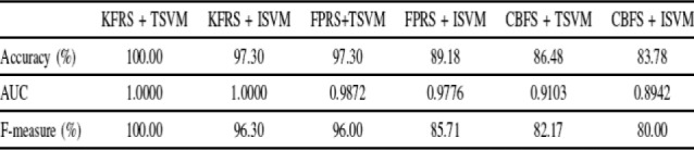
Comparison of the different methods using the training set of size 38 for miRNA dataset.

FIGURE 4.

ROC curves for different combination of methods.

E. Biological Relevance

The biological relevance of the miRNA biomarkers has been studied. First, we have identified validated target genes of five miRNAs using miRWalk database available at http://www.umm.uni-heidelberg.de/apps/zmf/mirwalk/. Thereafter, we have put these validated target genes into DAVID software available at http://david.abcc.ncifcrf.gov/ as input to find the KEGG pathways. In this way we have identified 64 significant pathways (-value <0.05). Furthermore, known cancer associations with the miRNAs obtained from the recently published cancer-miRNA network [2] and miRcancer database available at http://mircancer.ecu.edu. are also reported in Table 6. It is quite interesting to observe that all the selected markers are found to be associated with several types of cancer. For example, hsa-miR-143 is involved in six types of cancer found from the cancer miRNA network. Likewise, cancer types associated with four other miRNAs are found from the miRcancer database.

TABLE 6.

Cancer types associated with the microRNA markers obtained from the cancer miRNA network and miRNA cancer association database.

To study how the selected miRNA markers are involved in various biological activities, we have observed KEGG pathway enrichment of the target genes of each of the miRNAs using TargetScan 5 from DIANA LAB available at http://diana.cslab.ece.ntua.gr/mirPath. Table 7 shows the top five significant pathways for the target genes and corresponding -values as obtained from the database of DIANA LAB. It can be seen that the KEGG signaling pathway terms (for example, T cell receptor signaling pathway) are associated with the four miRNA markers. This signifies that the selected miRNA markers are indeed involved in different cancer pathways. When one of the proteins in the pathway is mutated, it can be stuck in the “on” or “off” position, which is a necessary step in the development of many cancers. Moreover, some more specific pathways are noticed within the top five significant pathways of the miRNA markers. For example, hsa-miR-143 have target genes that are involved in the pathways of colorectal and prostate cancers (-value: 8.19e-05 and 1.27e-04, respectively). There are specific cancer pathways for the miRNAs. These are Melanoma (-value: 5.31e-04) for hsa-miR-143 and Glioma (-value: 1.30e-03) for hsa-miR-30e. The pathway for renal cell carcinoma (-value: 6.10e-03) is found for hsa-miR-185. These results indicate that the selected miRNA markers are highly involved in different cancer pathways, suggesting that these are significant miRNA cancer markers.

TABLE 7.

Top 5 significant KEGG pathways as discovered using the database of DIANA lab.

VI. Conclusion

In this article, we have developed a novel classification model to explore gene and miRNA cancer datasets using KFRS followed by semisupervised prediction of cancer markers. The novelty of this work is two-fold. First, we have demonstrated that KFRS is capable to extract useful biomarkers both from gene and miRNA expression datasets. Second, we have shown that semisupervised learning approach improves prediction performance with respect to the well-known supervised algorithms.

Experimental results on the gene-expression as well as miRNA datasets of different tissue types, viz, colon, kidney, prostate, uterus, lung and breast have been demonstrated. In addition, the identified miRNA signatures are found to be involved with different types of cancer according to the recent literatures. Finally, a pathway enrichment study has been conducted that reveals that target genes of the selected miRNAs are involved in many cancer pathways. This method can also be used for finding cancer markers from other microRNA and gene expression data.

Microarray analysis has the potential to predict therapy response or survival. Class prediction gives the clinician an unbiased method to predict cancers instead of traditional methods based on histopathology or empirical clinical data, which do not always reflect patient outcome. Therefore, it is necessary to focus more on class prediction because of its potential to influence the clinical management of cancer. However, microarray data are high dimensional, characterized by many variables and few observations. Moreover, this technique suffers from a low signal-to-noise ratio, which causes instability in gene signatures. Hence, to improve prediction accuracy, efficient dimensionality reduction techniques need to be explored. Furthermore, inadequate observations of gene/miRNA data result in poor performance of the traditional supervised methods. This necessarily entails the use of effective semisupervised methods in order to improve prediction accuracy. Our proposed method that considers both the approaches, can be used to guide the clinical/translational management of cancer and other diseases.

As a scope of further development, several issues remain open to be addressed: 1) integration of other sources of information could be important to enhance clinical/translational research. For example, model development where both clinical variables and gene/miRNA expression can be combined to improve prediction power; 2) different combination of feature selection methods needs to be investigated to obtain more biologically relevant genetic signatures and 3) the concept of fuzzy set theory could be introduced in semisupervised learning to improve model development.

Biographies

Debasis Chakraborty received the bachelor’s degree in electronics and telecommunication from the University of Calcutta, Kolkata, India, in 1990. He worked in different companies in India from 1990 to 1999. He received the master’s degree in computer science and engineering from Bengal Engineering College (Deemed University), Howrah, India, in 2003. He is currently an Associate Professor with the Department of Electronics and Communication Engineering, Murshidabad College of Engineering and Technology, Baharampur, India. His research interests include supervised and semisupervised learning, pattern classification, remote sensing, and bioinformatics.

Ujjwal Maulik (M’99–SM’05) has been a Professor with the Department of Computer Science and Engineering, Jadavpur University, Kolkata, India, since 2004. He received the bachelor’s degree in physics and computer science, in 1986 and 1989, respectively, and the master’s and Ph.D. degrees in computer science, in 1992 and 1997, respectively. He was the Chair of the Department of Computer Science and Technology, Kalyani Government Engineering College, Kalyani, India, from 1996 to 1999. He was with the Los Alamos National Laboratory, Los Alamos, NM, USA, in 1997, the University of New South Wales, Sydney, NSW, Australia, in 1999, the University of Texas at Arlington, Arlington, TX, USA, in 2001, the University of Maryland at Baltimore, Baltimore, MD, USA, in 2004, the Fraunhofer Institute for Autonomous Intelligent Systems, Sankt Augustin, Germany, in 2005, Tsinghua University, Beijing, China, in 2007, the University of Rome, Rome, Italy, in 2008, the University of Heidelberg, Heidelberg, Germany, in 2009, the German Cancer Research Center, Heidelberg, in 2010, 2011, and 2012, the Grenoble Institute of Technology, Grenoble, France, in 2010, 2013, and 2014, ICM, Warsaw, Poland, the University of Warsaw, Warsaw, in 2013, the International Center of Theoretical Physics (ICTP), Trieste, Italy, in 2014, and the University of Padua, Padua, Italy, in 2014. He has also visited many institutes/universities around the world for invited lectures and collaborative research. He has been invited to supervise the Ph.D. students in the well-known university in France. He has co-authored seven books and over 250 research publications. He was the recipient of the Government of India BOYSCAST Fellowship Award in 2001, the Alexander Von Humboldt Fellowship Award for Experienced Researchers in 2010, 2011, and 2012, and the Senior Associateship Award of ICTP, Italy, in 2012. He coordinates five Erasmus Mundus Mobility with Asia programs (European-Asian mobility program). He has been the Program Chair, the Tutorial Chair, and a program Committee Member of many international conferences and workshops. He is the Associate Editor of the IEEE Transactions on Fuzzy Systems and Information Sciences, and is also on the Editorial Board of many journals, including Protein and Peptide Letters. In addition, he has served as the Guest Co-Editor of special issues of journals, including the IEEE Transactions on Evolutionary Computation. He is the Founding Member of the IEEE Computational Intelligence Society Chapter, Kolkata Section, India, and was a Secretary and Treasurer in 2011, the Vice Chair in 2012, and the Chair in 2013 and 2014. He is a fellow of the Indian National Academy of Engineering, the West Bengal Association of Science and Technology, the Institution of Engineering and Telecommunication Engineers, and the Institution of Engineers. His research interests include computational intelligence, bioinformatics, combinatorial optimization, pattern recognition, and data mining.

References

- [1].Berezikov E., Cuppen E., and Plasterk R. H. A., “Approaches to microRNA discovery,” Nature Genet., vol. 38, pp. S2–S7, May 2006. [DOI] [PubMed] [Google Scholar]
- [2].Bandyopadhyay S., Mitra R., Maulik U., and Zhang M. Q., “Development of the human cancer microRNA network,” BMC Silence, vol. 1, no. , p. 6, 2010. [DOI] [PMC free article] [PubMed] [Google Scholar]
- [3].Bandyopadhyay S., Mukhopadhyay A., and Maulik U., “An improved algorithm for clustering gene expression data,” Bioinformatics, vol. 23, no. 21, pp. 2859–2865, 2007. [DOI] [PubMed] [Google Scholar]
- [4].Maulik U., Mukhopadhyay A., and Bandyopadhyay S., “Combining Pareto-optimal clusters using supervised learning for identifying co-expressed genes,” BMC Bioinformat., vol. 10, no. 1, p. 27, 2009. [DOI] [PMC free article] [PubMed] [Google Scholar]
- [5].Mukhopadhyay A., Bandyopadhyay S., and Maulik U., “Multi-class clustering of cancer subtypes through SVM based ensemble of Pareto-optimal solutions for gene marker identification,” PLoS ONE, vol. 5, no. 11, p. e13803, 2010. [DOI] [PMC free article] [PubMed] [Google Scholar]
- [6].Maulik U. and Mukhopadhyay A., “Simulated annealing based automatic fuzzy clustering combined with ANN classification for analyzing microarray data,” Comput. Oper. Res., vol. 37, no. 8, pp. 1369–1380, Aug. 2010. [Google Scholar]
- [7].Mukhopadhyay A. and Maulik U., “Towards improving fuzzy clustering using support vector machine: Application to gene expression data,” Pattern Recognit., vol. 42, no. 11, pp. 2744–2763, Nov. 2009. [Google Scholar]
- [8].Maulik U., “Analysis of gene microarray data in a soft computing framework,” Appl. Soft Comput., vol. 11, no. 6, pp. 4152–4160, Sep. 2011. [Google Scholar]
- [9].Maulik U., Bandyopadhyay S., and Mukhopadhyay A., Multiobjective Genetic Algorithms for Clustering: Applications in Data Mining and Bioinformatics. New York, NY, USA: Springer-Verlag, 2011. [Google Scholar]
- [10].Bandyopadhyay S., Maulik U., and Wang J. T., Analysis of Biological Data: A Soft Computing Approach. Singapore: World Scientific, 2007. [Google Scholar]
- [11].Luo L.-K., Huang D.-F., Ye L.-J., Zhou Q.-F., Shao G.-F., and Peng H., “Improving the computational efficiency of recursive cluster elimination for gene selection,” IEEE Trans. Comput. Biol. Bioinformat., vol. 8, no. 1, pp. 122–129, Jan-Feb 2011. [DOI] [PubMed] [Google Scholar]
- [12].Keller A., Schummer M., Hood L., and Ruzzo W., “Bayesian classification of DNA array expression data,” Univ. Washington, Seattle, WA, USA, Tech. Rep. UW-CSE-2000-08-01, 2000. [Google Scholar]
- [13].Friedman N., Linial M., Nachman I., and Peer D., “Using Bayesian networks to analyze expression data,” J. Comput. Biol., vol. 7, nos. 3–4, pp. 601–620, 2000. [DOI] [PubMed] [Google Scholar]
- [14].Kelemen A., Zhou H., Lawhead P., and Liang Y., “Naive Bayesian classifier for microarray data,” in Proc. IEEE Int. Conf. Neural Netw., vol. 3 Jul. 2003, pp. 1769–1773. [Google Scholar]
- [15].Chen H.-Y., et al. , “A five-gene signature and clinical outcome in non-small-cell lung cancer,” New England J. Med., vol. 356, no. 1, pp. 11–20, Jan. 2007. [DOI] [PubMed] [Google Scholar]
- [16].Pochet N., Smet F. D., Suykens J. A. K., and Moor B. L. R. D., “Systematic benchmarking of microarray data classification: Assessing the role of non-linearity and dimensionality reduction,” Bioinformatics, vol. 20, no. 17, pp. 3185–3195, Jul. 2004. [DOI] [PubMed] [Google Scholar]
- [17].Ramaswamy S., et al. , “Multiclass cancer diagnosis using tumor gene expression signatures,” Proc. Nat. Acad. Sci., vol. 98, no. 26, pp. 15149–15154, 2001. [DOI] [PMC free article] [PubMed] [Google Scholar]
- [18].Berrar D., Bradbury I., and Dubitzky W., “Instance-based concept learning from multiclass DNA microarray data,” BMC Bioinformat., vol. 7, no. 1, p. 73, 2006. [DOI] [PMC free article] [PubMed] [Google Scholar]
- [19].Prasad N. B., et al. , “Identification of genes differentially expressed in benign versus malignant thyroid tumors,” Clin. Cancer Res., Off. J. Amer. Assoc. Cancer Res., vol. 14, no. 11, pp. 3327–3337, 2008. [DOI] [PMC free article] [PubMed] [Google Scholar]
- [20].Chapelle O., Sindhwani V., and Keerthi S. S., “Optimization techniques for semi-supervised support vector machines,” J. Mach. Learn. Res., vol. 9, pp. 203–233, Jan. 2008. [Google Scholar]
- [21].Käll L., Canterbury J. D., Weston J., Noble W. S., and MacCoss M. J., “Semi-supervised learning for peptide identification from shotgun proteomics datasets,” Nature Methods, vol. 4, pp. 923–925, Oct. 2007. [DOI] [PubMed] [Google Scholar]
- [22].Weston J., Ie E., Zhou D., Elisseeff A., Noble W. S., and Leslie C., “Semi-supervised protein classification using cluster kernels,” Bioinformatics, vol. 21, no. 15, pp. 3241–3247, 2008. [DOI] [PubMed] [Google Scholar]
- [23].Ernst J., Beg Q. K., Kay K. A., Balázsi G., Oltvai Z. N., and Bar-Joseph Z., “A semi-supervised method for predicting transcription factor-gene interactions in Escherichia coli,” PLoS Comput. Biol., vol. 4, p. e1000044, Mar. 2008. [DOI] [PMC free article] [PubMed] [Google Scholar]
- [24].Maulik U., Mukhopadhyay A., and Chakraborty D., “Gene-expression-based cancer subtypes prediction through feature selection and transductive SVM,” IEEE Trans. Biomed. Eng., vol. 60, no. 4, pp. 1111–1117, Apr. 2013. [DOI] [PubMed] [Google Scholar]
- [25].Maulik U. and Chakraborty D., “Fuzzy preference based feature selection and semisupervised SVM for cancer classification,” IEEE Trans. Nanobiosci., vol. 13, no. 2, pp. 152–160, Jun. 2014. [DOI] [PubMed] [Google Scholar]
- [26].Koestler D. C., et al. , “Semi-supervised recursively partitioned mixture models for identifying cancer subtypes,” Bioinformatics, vol. 26, no. 20, pp. 2578–2585, 2010. [DOI] [PMC free article] [PubMed] [Google Scholar]
- [27].Steinfeld I., Navon R., Ardigò D., Zavaroni I., and Yakhini Z., “Clinically driven semi-supervised class discovery in gene expression data,” Bioinformatics, vol. 24, no. 16, pp. 190–197, 2008. [DOI] [PubMed] [Google Scholar]
- [28].Bair E. and Tibshirani R., “Semi-supervised methods to predict patient survival from gene expression data,” PLoS Biol., vol. 2, pp. 511–522. [DOI] [PMC free article] [PubMed] [Google Scholar]
- [29].Huang H. and Feng H., “Gene classification using parameter-free semi-supervised manifold learning,” IEEE Trans. Comput. Biol. Bioinformat., vol. 9, no. 3, pp. 818–827, May-Jun 2012. [DOI] [PubMed] [Google Scholar]
- [30].Rajapakse J. C. and Mundra P. A., “Multiclass gene selection using Pareto-fronts,” IEEE Trans. Comput. Biol. Bioinformat., vol. 10, no. 1, pp. 87–97, Jan-Feb 2013. [DOI] [PubMed] [Google Scholar]
- [31].Hu Q., Yu D., Pedrycz W., and Chen D., “Kernelized fuzzy rough sets and their applications,” IEEE Trans. Knowl. Data Eng., vol. 23, no. 11, pp. 1649–1667, Nov. 2011. [Google Scholar]
- [32].Hu Q., Zhang L., Chen D., Pedrycz W., and Yu D.. Gaussian Kernel Based Fuzzy Rough Sets: Model, Uncertainty Measures and Applications. [Online]. Available: http://www4.comp.polyu.edu.hk/
- [33].Hu Q., Yu D., and Guo M., “Fuzzy preference based rough sets,” Inf. Sci., vol. 180, no. 10, pp. 2003–2022, 2010. [Google Scholar]
- [34].Dash M. and Liu H., “Consistency-based search in feature selection,” Artif. Intell., vol. 151, nos. 1–2, pp. 155–176, Dec. 2003. [Google Scholar]
- [35].Vapnik V. N., Statistical Learning Theory. New York, NY, USA: Wiley, 1998. [Google Scholar]
- [36].Tou J. T. and Gonzales R. C., Pattern Recognition Principles. Reading, MA, USA: Addison-Wesley, 1974. [Google Scholar]
- [37].Mitchel T. M., Machine Learning. New York, NY, USA: McGraw-Hill, 1997. [Google Scholar]
- [38].Schölkopf B., Burges C. J. C., and Smola A. J., Advances in Kernel Methods: Support Vector Learning. Cambridge, MA, USA: MIT Press, 1999. [Google Scholar]
- [39].Golub T. R., et al. , “Molecular classification of cancer: Class discovery and class prediction by gene expression monitoring,” Science, vol. 286, no. 5439, pp. 531–537, 1999. [DOI] [PubMed] [Google Scholar]
- [40].Peng H., Long F., and Ding C., “Feature selection based on mutual information criteria of max-dependency, max-relevance, and min-redundancy,” IEEE Trans. Pattern Anal. Mach. Intell., vol. 27, no. 8, pp. 1226–1238, Aug. 2005. [DOI] [PubMed] [Google Scholar]
- [41].Kreyszig E., Introductory Mathematical Statistics. New York, NY, USA: Wiley, 1970. [Google Scholar]
- [42].Olson D. L. and Delen D., Advanced Data Mining Techniques, 1st ed. Berlin, Germany: Springer-Verlag, 2008. [Google Scholar]
- [43].Liu H. and Setiono R., “Chi2: Feature selection and discretization of numeric attributes,” in Proc. 7th Int. Conf. Tools Artif. Intell., Herndon, VA, USA, Nov. 1995, pp. 388–391. [Google Scholar]
- [44].[Online]. Available: http://www.biolab.si/supp/bi-cancer/projections/
- [45].Lu J., et al. , “MicroRNA expression profiles classify human cancers, Nature, vol. 435, no. 7043, pp. 834–838, Jun. 2005. [DOI] [PubMed] [Google Scholar]
- [46].Hsu C., Chang C., and Lin C. (2013). A Practical Guide to Support Vector Classification. [Online]. Available: http://www.csie.ntu.edu.tw~cjlin/
- [47].Hollander M. and Wolfe D. A., Nonparametric Statistical Methods. NJ, USA: Wiley, 1999. [Google Scholar]
- [48].Bradley A. P., “The use of the area under the ROC curve in the evaluation of machine learning algorithms,” Pattern Recognit., vol. 30, no. 7, pp. 1145–1159, Jul. 1997. [Google Scholar]