A controlled statistical study to assess measurement variability as a function of test object position and configuration for automated surveillance in a multicenter longitudinal COPD study (SPIROMICS)

Abstract

Purpose:

A test object (phantom) is an important tool to evaluate comparability and stability of CT scanners used in multicenter and longitudinal studies. However, there are many sources of error that can interfere with the test object-derived quantitative measurements. Here the authors investigated three major possible sources of operator error in the use of a test object employed to assess pulmonary density-related as well as airway-related metrics.

Methods:

Two kinds of experiments were carried out to assess measurement variability caused by imperfect scanning status. The first one consisted of three experiments. A COPDGene test object was scanned using a dual source multidetector computed tomographic scanner (Siemens Somatom Flash) with the Subpopulations and Intermediate Outcome Measures in COPD Study (SPIROMICS) inspiration protocol (120 kV, 110 mAs, pitch = 1, slice thickness = 0.75 mm, slice spacing = 0.5 mm) to evaluate the effects of tilt angle, water bottle offset, and air bubble size. After analysis of these results, a guideline was reached in order to achieve more reliable results for this test object. Next the authors applied the above findings to 2272 test object scans collected over 4 years as part of the SPIROMICS study. The authors compared changes of the data consistency before and after excluding the scans that failed to pass the guideline.

Results:

This study established the following limits for the test object: tilt index ≤0.3, water bottle offset limits of [−6.6 mm, 7.4 mm], and no air bubble within the water bottle, where tilt index is a measure incorporating two tilt angles around x- and y-axis. With 95% confidence, the density measurement variation for all five interested materials in the test object (acrylic, water, lung, inside air, and outside air) resulting from all three error sources can be limited to ±0.9 HU (summed in quadrature), when all the requirements are satisfied. The authors applied these criteria to 2272 SPIROMICS scans and demonstrated a significant reduction in measurement variation associated with the test object.

Conclusions:

Three operator errors were identified which significantly affected the usability of the acquired scan images of the test object used for monitoring scanner stability in a multicenter study. The authors’ results demonstrated that at the time of test object scan receipt at a radiology core laboratory, quality control procedures should include an assessment of tilt index, water bottle offset, and air bubble size within the water bottle. Application of this methodology to 2272 SPIROMICS scans indicated that their findings were not limited to the scanner make and model used for the initial test but was generalizable to both Siemens and GE scanners which comprise the scanner types used within the SPIROMICS study.

1. INTRODUCTION

An increasing number of multicenter and longitudinal lung studies using CT scanners are relying on monthly scanning of the COPDGene phantom (CTP657: Phantom Laboratories, Salem, NY)¹ to monitor between scanner differences and the temporal stability of participant scanners. This procedure assumes that the CT scanner status can be obtained from the analysis of the resultant images, requiring that the test object must be scanned consistently, utilizing the same scan and reconstruction protocol as is used for the study being followed. While the header record embedded with each scan data set can be used to determine if the scan protocol has been followed exactly, there is less control over how well the test object has been positioned within the scanner. It is clear that there must be some parameters set for acceptance of a scan based upon proper positioning of the test object within the scan field. For instance, it is unacceptable to have the object lying face down on the table pad when the scan protocol called for the object to be upright with the two faces of the object parallel with the scan plane. However it is less clear that whether a scan shall be accepted or rejected when the test object face is just a few degrees off of parallel to the scan plane and/or when the water bottle has been offset in the object after refilling. To establish standards for scan acceptance in the growing number of lung-based imaging studies utilizing the COPDGene test object or similar test objects, we evaluated the role of object angle relative to the scan plane when using the object for monitoring intrascanner and interscanner consistencies in a multicenter longitudinal study. To test this we utilized scans on a single scanner where tilt angle was adjusted through a range of settings as well as the multisite, longitudinal data sets obtained by the subpopulations and intermediate outcome measures in COPD study (SPIROMICS).² From the resultant observations, we provided acceptance guidelines for each type of test object variance.

2. METHODOLOGY

The COPDGene test object has been discussed in detail elsewhere.¹ In summary, it consists of an outer, water-equivalent ring (7–20 HU) and an inner lung equivalent (−856 HU) foam with various embedded objects including a water bottle, an empty (air filled) cylinder, and a 30 mm diameter acrylic rod. In addition the test object has tubes of various wall thicknesses simulating bronchial segments. This paper evaluates the density measures (CT number on the Hounsfield scale) derived from the water bottle, the air filled cylinder, the acrylic rod, the lung equivalent foam, and air outside the test object in addition to the metrics derived from the simulated airway segments. Customized protocols have been established with adjustments made for different size (body mass index: BMI) ranges of the human subjects being scanned. Scanning of the test object followed the protocol used by SPIROMICS for a subject with a medium BMI imaged at total lung capacity. The protocol varies for various make and model scanners, targeting a specific computed tomography dose index-volume (CTDI_vol), to match the target scan obtained on a Siemens Flash scanner utilizing 120 kV, 110 mAs, pitch = 1, slice thickness = 0.75 mm, and slice spacing = 0.5 mm. For the purposes of this phantom study, we used a fixed display field of view (dFOV) of 365 mm.

2.A. Image processing

2.A.1. Density measurement

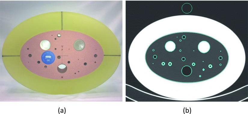
The test object image was segmented into various regions (Fig. 1). The 30 mm air, water, acrylic regions and the elliptical lung foam region were separated using a thresholding method followed by a connected component analysis method,³ which identifies each separated object and assigns each with a unique label. The cylindrical holes and tubes (airways) that were embedded inside the lung foam were excluded from the foam region. The outside air was sampled by a 30 mm cylinder in the center of the top pure air region outside of the test object, 5 mm away from the outer edge of the object. The segmented depth (z-axis) was 20 mm and located in the center of the test object. Next, the five regions of interest (lung, 30 mm inside air, water, acrylic, and outside air regions) were further eroded from both ends down to 10 mm for density evaluation. While all other regions were centered on the initial 20 mm length based upon the ends of the test object, the water sample location was chosen to be within the central 20 mm’s based upon the ends of the water bottle, since the water bottle might be erroneously positioned within the test object by the technician in charge of refilling the bottle. The segmented regions were further eroded by 4 pixels (or 2.85 mm with our SPIROMICS test object protocol) from the inner/outer edge in the x–y plane to eliminate the partial volume effect near the boundaries. Within the final eroded volume of interest (VOI), the mean and standard deviations were then evaluated.

FIG. 1.

(a) COPDGene phantom (CTP657). (b) Segmented regions of interest.

2.A.2. Airway measurement

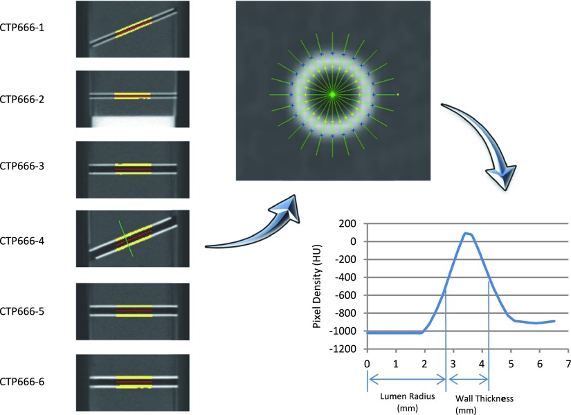
Six embedded airway tubes were segmented from the lung foam in the above stage and their centerlines were identified. As demonstrated in Fig. 2, the tubes were then numerically sectioned into slices perpendicular to their centerlines. At each tube location, a set of rays were defined, which radiated from the center point and the density along each ray formed a brightness profile.^4,5 The full width at half maximum method, or FWHM, was used to identify the inner and outer boundaries of the airway wall.⁶ The averaged lumen radius and wall thickness from each tube cross section was used to characterize airway tube metrics. The FWHM method does not define the true tube dimensions but rather represents the degree to which the wall representation is spread spatially and serves as an index related to the scanner point spread function, free of image processing biases in the postprocessing step to measure the tube dimension.

FIG. 2.

Airway measurement process. Left: six embedded airways are segmented. Upper right: on a perpendicular section of an airway, a set of rays are radiated from the center point. Lower right: FWHM method is used to evaluate the brightness profile along a ray.

2.A.3. MTF measurement

MTF measurement was always done at the edge of acrylic rod using a similar method as described in Refs. ⁷ and ⁸. The acrylic insert (15 mm in radius) and its surrounding regions were used to produce an edge spread function (ESF). First, on each 2D slice, the pixels in a ring area between 5 and 25 mm from the acrylic center (or 10 mm away from its edge on each side) were transformed into a parametric line function based on their distance from the edge of the acrylic disk. This would yield a nonuniformly sampled ESF. Then linear interpolation was used to resample the ESF, with bins of one-tenth that of the in-plane pixel size, and a uniformly resampled ESF was produced. The ESF was differentiated to produce the line-spread function (LSF), which was multiplied by a Hann window to remove the noise in the tails. The width of the Hann window matched the length of ESF. Then, the fast Fourier transform (FFT) of the LSF yielded the MTF. Finally, we averaged the MTF calculated on all 2D slices to produce the final MTF.

2.A.4. Tilt angle detection

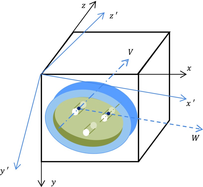
Two vectors one presented by the center line of the 30 mm acrylic rod (vector V in Fig. 3) and the other one pointed from the 3D center of the acrylic rod to the 3D center of the water bottle (vector W) together define the 3D orientation of the test object, where the latter vector was actually calculated from the vector pointed from the 3D center of the acrylic rod to the 3D center of the 30 mm air hole to avoid the possible air bubble effect in the water bottle. Based on these two measured vectors, the orthogonal coordinating axes of the tilted system, x′y′z′, were identified, as shown in Fig. 3. Axes z′ and x′ are parallel to vectors V and W, respectively.

FIG. 3.

Test object in tilt position. Three cylinder structures shown at top left, top right, and bottom are acrylic rod, water bottle, and air hole, respectively.

Next, the accurate tilt angles around all three axes were calculated using the same method whose idea was proposed in Ref. 9 and an implementation was described in Ref. 10. The only difference is that our coordinate system is different than theirs, so we reformatted the formulas to match our right-handed coordinate system.

2.A.5. Water bottle offset detection

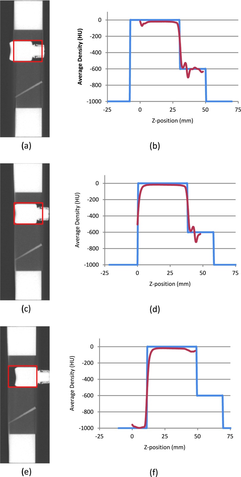
The water bottle is a movable component in the test object. It is required that the bottom of the bottle be aligned with the end plane of the test object during scanning, so that a sagittal image, as shown in Fig. 4(c), can be obtained. However, noticeable offset of the water bottle is frequently observed in practice, and some of the offsets are as severe as shown in Figs. 4(a) and 4(e). The offset value is defined as the relative position of the water bottom compared to the test object’s end plane. A negative value is given to Fig. 4(a), and a positive value is assigned to Fig. 4(e).

FIG. 4.

Detecting water bottle position.

In order to locate the water bottle position, the original image was first rotated back to the standard position by the detected tilt angle. Next, the cylinder center, which holds the water bottle, was located based on its known nominal position. At each slice within the cylinder region (see the red rectangle mark on the sagittal section image, left side in Fig. 4), the average pixel density was calculated. A measured density curve along a z-axis was thus produced (see the red curve in the right side in Fig. 4). The end plane of the test object, where the start point of the measured density distribution curve was located, was used as the reference point and marked as position 0 mm in the figure.

Next, two nominal density distribution curves were constructed based on the known water bottle dimension for two possible facing directions, respectively (the blue curve in Fig. 4 is for one of such directions in which the bottle neck is pointing to the right). The least squares method was used to register each of these two curves with the measured curve separately. The one that had the minimum fitting error was defined as the direction of the water bottle and the rising edge of blue curve was located as the bottom of the water bottle. In the examples given in Fig. 4, the detected water bottle offset was approximately −8, 0, and 12 mm for the three cases (top to bottom), respectively.

2.A.6. Air bubble size detection

After the water bottle was precisely located along the z-axis, its main body could be identified by excluding the slices where its neck and bottom cave-in might be affected. Within the overlap region of the main body and the segmented 20 mm slices, pixels labeled as “Air” were counted and converted to volume with the known physical size of pixel.

2.B. Scanning studies

Two kinds of experiments were carried out in this study. The first one consisted of three subexperiments. A COPDGene test object was scanned using a dual source multidetector computed tomographic scanner (Siemens Somatom Flash) with the SPIROMICS inspiration protocol (120 kV, 110 mAs, pitch = 1, slice thickness = 0.75 mm, slice spacing = 0.5 mm, reconstruction diameter = 365 mm) to evaluate the effects of tilt angle, water bottle offset, and air bubble size. After analysis of the results, a guideline was reached to achieve more reliable results for COPDGene test object.

Next we applied the above finding to the 2272 COPDGene test object scans collected over four years in the SPIROMICS study. We compared changes of the data consistency before and after excluding the scans that fell out of the guideline.

2.B.1. Measurement affected by tilt angle

The COPDGene test object was scanned using varying tilt angles around three orthogonal axes. The tilt of the test object was manually established by using a protractor to control the tilt angle between the corresponding alignment lines marked on the test object and the alignment laser line projected from the CT scanner. Once the desired tilt angle was approximately reached, the test object was then fastened on the scanner bed with tape before proceeding with the scanning. Absolute tilt angles ranged between 0° and 8° for the x-axis, 0° and 6° for the y-axis, and 0° and 7° for the z-axis. A total of 266 different tilt combinations were gathered. Three scans were acquired at each position. Density measurements, airway measurements, and MTF curves were calculated. Tilt around the z-axis was found to not significantly affect the measurements. To simplify the analysis, we composed the effects of tilt angle around the x-axis and y-axis together to a single item, called tilt index,

$${\displaystyle \text{Tilt Index}=\frac{\left|\theta \right|}{arctan\left(\frac{30}{250}\right)}+\frac{\left|\psi \right|}{arctan\left(\frac{30}{350}\right)}=\frac{\left|\theta \right|}{6.84}+\frac{\left|\psi \right|}{4.90},}$$ (1)

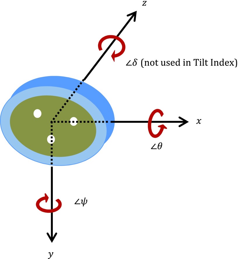
where 250 and 350 mm are the lengths of the shorter and longer axes, respectively, for the oval shaped test object. 30 mm is the maximum tilt offset to keep the central 20 mm thick sampling slab within the region of the 50 mm thick of test object. θ and ψ are the tilt angles around the x-axis and y-axis, respectively, as shown in Fig. 5. The constant values 6.84 and 4.90 have the units of degree.

FIG. 5.

Tilt angle around three axes.

We used a generalized additive mixed-effects model (GAMM) to measure the effect of tilt index on the mean densities of the five materials and constructed a measurement of variation induced by tilt index, as detailed in Appendix A.

2.B.2. Measurement affected by water bottle position

The test object was scanned at a standard orientation using 29 different water bottle positions, offset from −8 to 16 mm. Three scans were gathered for each position. Density measurements, airway measurements, and MTF curves (measured at the edge of acrylic rod) were calculated. We used a similar model to analyze the effects of the water bottle position on water mean density, as detailed in Appendix B.

2.B.3. Measurement affected by air bubble size

The test object was scanned at standard orientation, standard water bottle position (i.e., offset = 0 mm), with 32 different air bubble sizes. To produce various sized air bubbles, we took half of the water out of a fully filled water bottle with a syringe and then refilled the water bottle with the water from that syringe by 32 steps. At the end of each step, the amount of water left in the syringe, which can be read from the syringe scale, revealed the proximately air bubble size produced in the water bottle. Three repeat scans were acquired for each group. Density measurements, airway measurements, and MTF curves (measured at the edge of acrylic rod) were calculated.

2.B.4. Filtering SPIROMICS test object scans with acceptability criteria

SPIROMICS used the COPDGene test objects to evaluate the consistency of all participant CT scanners. Over four years, 2272 valid 3D images were collected using the SPIROMICS CT protocol, on 24 scanners (ten different scanner types from two manufactures: Siemens and GE) residing at 13 SPIROMICS centers.

Based upon the findings from the above discussed test scans on the Iowa research CT scanner, the combined requirement for scan acceptability was tilt index ≤0.3, water bottle offset within [−6.6, 7.4], and no detectable air bubble. By using such guidelines to filter the acceptable test object scans in the SPIROMICS study, we hypothesized that the variations in test object measurements would be reduced. Appendix C described the detailed statistical test procedure.

3. RESULTS

3.A. Measurement affected by tilt angle

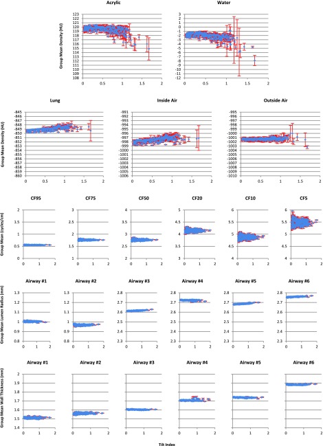
Following Sec. 2.B.1, the results of the measurements at each tilt index are shown in Fig. 6. The within-group averages over three repeat experiments for each fixed set of tilt angles were drawn as blue diamonds with the standard deviations shown as error bars in red.

FIG. 6.

Variation of the measurements with tilt index change. First two rows are density results for five materials. Third row is the MTF measurement results for the critical frequency (CF) at 95%, 75%, 50%, 20%, 10%, and 5% modulation, respectively. Last two rows are airway results. Blue diamonds indicate the within-group averages with standard deviations shown as error bars in red.

It is clear from Fig. 6 that both the location and the dispersion (scale) of the density measurement (rows 1 and 2) varied substantially with the tilt index, across the five materials of interest. However the MTF (3rd row) and airway measurements (4th and 5th rows) were sparsely affected by variations in the tilt index. It is also noticeable that once the tilt index went beyond 1.0, the standard deviation of the density measurements for some materials increased rapidly, implying that the repeatability became worse and the results were less trustworthy. Thus we excluded all density measurements with tilt index exceeding 1.0 in magnitude from the statistical analyses reported below.

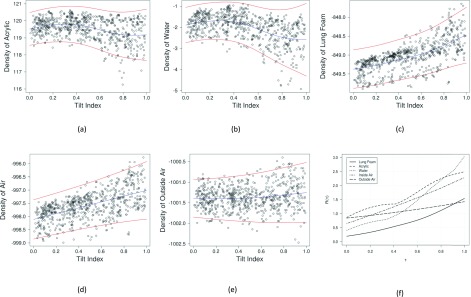
In Figs. 7(a)–7(e), we plotted the observed mean density data, the smooth function fits, and the 95% prediction limits for the five materials (which incorporated the additional uncertainty due to the random group effects). For each subplot, the blue curve showed the smooth function fits and the two red curves indicated the lower and upper prediction limits, respectively. Note that $R\left(\tau \right)$ defined in Eq. (A2) is the “cumulative” range of the 95% prediction intervals for tilt index up to τ, which is an increasing function of τ. Figure 7(f) plots R(τ) against τ, for each of the five materials. From these plots, we observe that the density variation range at τ = 0.3 is 1.3, 0.8, 0.4, 1.1, and 1.0 HU for acrylic, water, lung, inside air, and outside air, respectively. Thus at any tilt index lower than 0.3, we can be 95% confident that the density variation range of any of the five materials is no more than 1.3 HU.

FIG. 7.

Original data (open circle), smooth function fits (blue curve), and the 95% prediction limits (two red curves) for the densities of the five materials [(a)–(e)] and the function plots of R(τ) vs. τ ∈ [0, 1] for the five materials (f).

3.B. Measurement affected by water bottle position

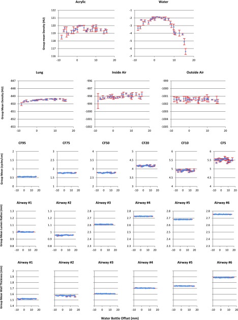
The results of the measurements at each bottle position (from Sec. 2.B.2) are shown in Fig. 8. The layout of Fig. 8 is similar to Fig. 6. It is easy to see that within all three categories, all measurements were very stable with the change of water bottle position, except the water density measurements.

FIG. 8.

Variation of the measurements with the change of the water bottle offset. First two rows are density results for five materials. Third row is the MTF measurement results. Last two rows are airway results. Blue diamonds indicate the within-group averages with standard deviations shown as error bars in red.

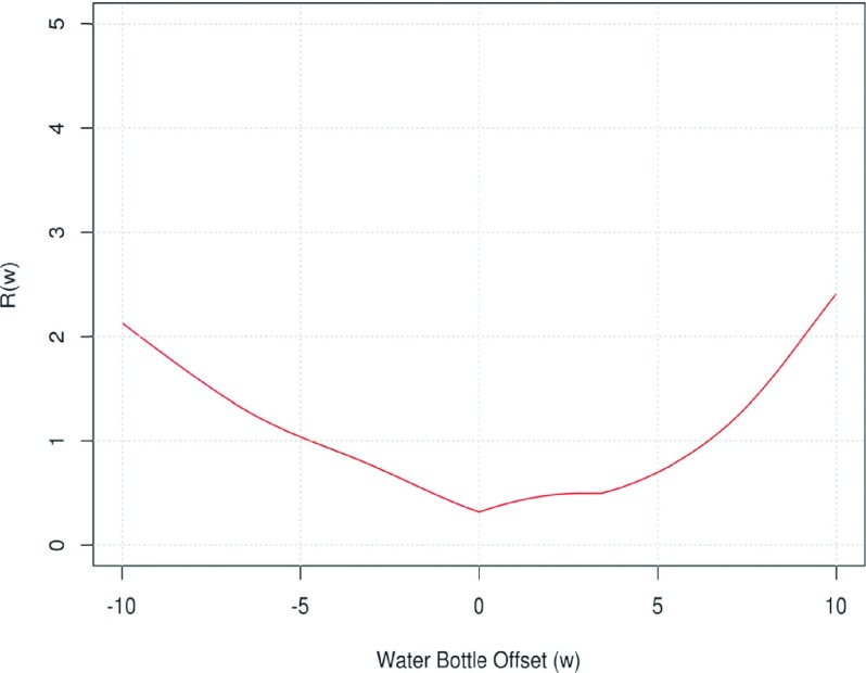
Figure 9 showed the function R(w) defined in the same manner as in Eq. (A2), i.e., it is the cumulative range of the prediction intervals for the water bottle offset between 0 and w for w > 0 or between w and 0 if w < 0. It can be checked that R(w) ≤ 1.3 HU, over the interval [−6.6 mm, 7.4 mm].

FIG. 9.

Plot of the function for water bottle offset analysis.

3.C. Measurement affected by air bubble size

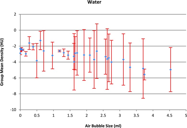
To summarize the results from Sec. 2.B.3, within all three categories, all measurements were very stable with the change of air bubble size, except the measurement for the density of water. As shown in Fig. 10, the mean water density became unstable when there was an existing air bubble. The big within-group standard deviation also shows that the repeatability was lost when air bubble was present.

FIG. 10.

Water density changes with air bubble size. Diamonds indicate the within-group averages with scale shown on the left y-axis. Blue diamonds indicate the within-group averages with standard deviations shown as error bars in red.

3.D. Filtering SPIROMICS test object scans with acceptability criteria

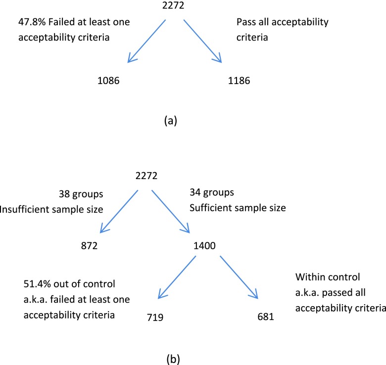
Here we report the test result for the 2272 SPIROMICS test object scans by applying the filtering criteria, as discussed in Sec. 2.B.4. Out of the 2272 scans, the percentage of the scans that failed to pass the acceptability criterion for tilt index, water bottle position, and air bubble size were 8.2%, 12.7%, and 36.1%, respectively. Altogether, 47.8% of the data failed to pass the acceptability criteria, as indicated in Fig. 11(a). To carry out the test, the 2272 scans were grouped by scanner, x-ray tube current, and kernel, resulting in 72 groups, 34 groups of which have adequate sample size and hence are used for the test. These 34 groups contain 1400 scans with 51.4% of data belonging to the out-of-control group, as demonstrated in Fig. 11(b).

FIG. 11.

Number of cases that passed/failed the acceptability criteria.

For the five materials (acrylic, water, lung, inside air, and outside air), the p-values for location and scale are listed in Table I. The results show that three materials (acrylic, water, and inside air) had at least one component (location or scale) significantly different between the control and out-of-control groups (in bold font, p-values < 0.05). We use median and median absolute deviation (MAD) to measure the location and scale for each group of data, respectively. The third row gives the mean of the difference between the medians of out-of-control and control samples for each group, and the fourth row gives the mean of the ratio between the MAD of out-of-control and control samples. The difference between the median and the ratio between MAD are described by the following formulas (both median and medDif are in unit of HU):

$${\displaystyle \mathrm{medDif}=\mathrm{median}\left(T_i\right)-\mathrm{median}\left(C_i\right),}$$

$${\displaystyle \mathrm{madDif}=\mathrm{MAD}\left(T_i\right)/\mathrm{MAD}\left(C_i\right).}$$

TABLE I.

Comparison between the control and out-of-control samples.

	Acrylic	Water	Lung	Inside air	Outside air
p-values for location	<0.0001	<0.0001	0.1399	0.0368	0.0954
p-values for scale	0.0657	0.0404	0.1245	0.1210	0.2012
Mean difference in location (medDif) (HU)	0.0719	−0.2370	0.0233	0.0591	0.0168
Mean ratio in scale (madDif)	1.1299	1.2501	1.4162	1.4536	1.3652

Furthermore, from the table, all the values for “mean ratio in scale” are greater than 1.0, which implies that the out-of-control samples are generally more variable than the control samples, and at least for water, where the difference was significant. The mean densities for acrylic, water, and inside air were significantly different between the control and out-of-control groups, while it was insignificant for lung-foam material. Densities of outside air for the two groups were not significantly different, which is expected.

4. DISCUSSION AND CONCLUSION

4.A. Create guideline to limit scanning imperfection

Results from Secs. 3.A–3.C demonstrate that the tilt angle, the water bottle offset, and the air bubble can all affect the accuracy of the measurement. It is a natural requirement to limit the variability of these parameters.

The water bottle can be easily filled free of air bubble by at least two methods: fill both the bottle and cap with water before closing it or submerge both parts into a bowl of water and close them underneath the water surface, which can be achieved with little effort.

From Fig. 10, it can be seen that even with a very small air bubble size (e.g., 0.03 ml), the density variation is close to 1 HU, compared with the no detectable air bubble case. The density value showed a random pattern with the size of air bubble and varied appreciably. Since it is very easy to eliminate air bubbles completely, we have recommended to simply insisting that the water portion of the test object be bubble free.

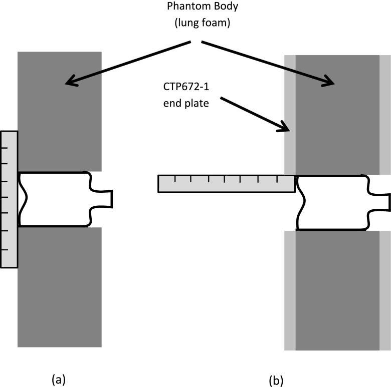
With the help of a ruler, the water bottle can be easily positioned with its base aligned with the test object end surface, as shown in Fig. 12. As seen in Panel (a), when there is no protective plate covering the phantom, the water bottle is placed up to the boundaries defined by the ruler. When there is a protective plate, a ruler is used to assure that the bottle is recessed no more than the thickness of the protective cover.

FIG. 12.

Methods for water bottle positioning.

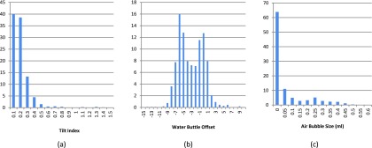
The tilt angle is the hardest part to control perfectly. From Fig. 7(f), we know that for most materials, the measurements are sensitive to the increasing tilt index. We try to set the threshold for tilt index to be as smaller as possible, yet while still being practical. We used four years of scans data acquired from the SPIROMICS project to find out how well the operator can control the tilt angle during scanning.

Figure 13(a) plots the histogram distribution of tilt index for 2272 SPIROMICS scans, which shows that 91.8% scans whose tilt index ≤0.3. That means, with a little bit effort on the operator side, the tilt index can be controlled no more than 0.3, which yields the maximum 1.3 HU (or ±0.65 HU) variation in 95% confidence interval for any material, from Fig. 7(f).

FIG. 13.

Distribution of tilt index, water bottle offset, and air bubble size in four years SPIROMICS scans. In all three figures, the unit of the vertical axis is “Percentage of Scans.”

The combined requirement is tilt index ≤ 0.3, −6.6 ≤ water bottle position ≤7.4, and no detectable air bubble. Assuming that perturbation due to tilt index and that due to water bottle position act independently, the combined prediction variance is the sum of the prediction variances due to the two sources of variations. Thus, with 95% confidence, the density measurement variation for all materials resulting from all three error sources can be limited to ±0.9 HU, when all the requirements are satisfied.

The 1.3 HU criteria for limiting the density variation caused by the tilt index and the 1.3 HU for limiting the density variation caused by the water bottle offset are both empirical values. A lower threshold would ensure less density variation but would make it harder to implement in practice based upon the offsets found to date. These values were chosen based on the trade-off between the performances and practicality. From the analysis of 2272 SPIROMICS test object, by applying these criteria, only 8.2% and 12.7% scans would be rejected for tilt index and water bottle offset, respectively. The trade-off is the desire to have zero variability and having a rejection rate that is on the order of 10%. It is expected that once automated rejections are implemented in such a study, errors in test object placement and configuration will significantly diminish.

4.B. Conclusion

This study evaluated the effects of test object tilt, water bottle position, and air bubble size. We demonstrate that the three types of operator error can significantly affect the usability of the acquired test object scan. Because of this, in order to obtain a stable longitudinal measurement, at the time of test object scan receipt at a radiology core laboratory, quality control procedures should include an assessment of the tilt index, the water bottle offset, and air bubble size.

With the availability of 2272 SPIROMICS scans, we performed a two-stage statistical test to evaluate the deterioration of data quality if the suggested guideline is not followed. As the data were collected from different scanners with various tube current and kernel configurations, we first grouped the data classified by scanner, current, and kernel, and for each group we performed a statistical evaluation. The results across different groups were then combined for further evaluation. The results indicate that our findings are not limited to the scanner make and model used to collect the test scans in this study but can be generalized across scanner types.

APPENDIX A: STATISTICAL MODEL FOR MEASUREMENT AFFECTED BY TILT ANGLE

In this section, we present the detailed statistical model to measure the effect of tilt index on the mean densities of the five materials and construct a measurement of variation induced by tilt index.

For each position of the data, three repetitive scans were performed and categorized as one group. As the three repetitive scans in each group receive identical treatment, their responses are likely correlated in that they share a common group-specific random component (technically referred to as random effect) which is assumed to be normally distributed, of zero mean and identical variance, and uncorrelated across groups, i.e., the b_g term in Eq. (A1) defined below.

To account for the fact that the tilt index does not uniquely determine the three tilt angles and other unknown confounding factors, we modeled the data by a GAMM.^11,12 Specifically, let y_g,i be the mean density of a particular material (acrylic, water, lung, inside air, or outside air) reconstructed from the scan taken at the ith replicate of the gth group of experiments and τ_g,i be the corresponding tilt index. We considered the following nonlinear mixed effects model for the variation in the mean density:

$${\displaystyle y_{g,i}=s\left({\tau }_{g,i}\right)+b_g+exp\left(c{\tau }_{g,i}\right)\sigma {\epsilon }_{g,i},}$$ (A1)

where s denotes some possibly nonlinear smooth function whose shape is estimated from the data, b_g denotes the random group effects, c and σ are unknown parameters, and ε_g,i’s are independent normal random variables of zero mean and unit variance, so that the within-group regression error is normally distributed of zero mean and standard deviation equal to $exp\left(c{\tau }_{g,i}\right)\sigma$. That the standard deviation specified to be an exponential function of the tilt index is motivated by Fig. 6 which suggests that the within-group scatter increases more or less exponentially with the tilt index. Thus, the within-group error standard deviation is σ for zero tilt index, but otherwise increases with the tilt index exponentially.

Model (A1) assumes that up to some group-specific random effects and random regression errors, the mean densities lie on a smooth function of the tilt index. It is possible to replace the smooth function of the tilt index by a smooth function of the three tilt angles. However, for ease of interpretation, we did not pursue the more complex model formulation. Model (A1) was fitted separately for each of the five materials, by the method of restricted maximum likelihood via the GAMM function in the r package mgcv. In particular, the estimated functions s are natural cubic splines.^11,12 Based on the fitted model for the density of a particular material, we found the largest tolerance limit for the tilt index within which, with 95% confidence, the mean density of that material differs from that at zero tilt index by no more than some prespecified value denoted by tol, which is set to be 0.65, as follows. First, for each tilt index τ ∈ [0, 1], we constructed the 95% prediction interval I(τ) = (l_τ, u_τ) for the mean density, with the formulas of the prediction limits given by

$${\displaystyle l_{\tau }=s\left(\tau \right)-1.96^{*}\hspace{0.17em}exp\left(c\tau \right)\sigma ,}$$

and

$${\displaystyle u_{\tau }=s\left(\tau \right)+1.96^{*}\hspace{0.17em}exp\left(c\tau \right)\sigma .}$$

Note that the variation due to the random group effects is omitted from the computation of the prediction interval because a relevant comparison keeps the specific group effect fixed.

Furthermore, we defined the cumulative range of the 95% prediction intervals for tilt index up to τ,

$${\displaystyle R\left(\tau \right)=\underset{t\in [0,\tau ]}{max}{u}_t-\underset{t\in \left[0,\tau \right]}{min}{l}_t,}$$ (A2)

which is an increasing function of τ.

Denote the largest tolerance limit by $\hat{\tau }$. The requirement on $\hat{\tau }$ is then equivalent to requiring that the union of all the 95% prediction intervals with $\tau \le \hat{\tau }$ lies inside an interval of length not more than twice tol, which is given by

$${\displaystyle \hat{\tau }=\arg \underset{\tau \in [0,\tau ]}{max}R\left(\tau \right)\le 2^{\ast }\hspace{0.17em}\mathrm{tol}.}$$ (A3)

APPENDIX B: STATISTICAL MODEL FOR MEASUREMENT AFFECTED BY WATER BOTTLE POSITION

For modeling the effect of the water bottle position on water mean density, we consider the following model similar to Eq. (A1):

$${\displaystyle y_{g,i}=s\left(p_{g,i}\right)+b_g+exp\left(c\right|p_{g,i}\left|\right)\sigma {\epsilon }_{g,i},}$$ (B1)

where y_g,i denotes the water mean density, s denotes some nonlinear smooth function, p_g,i denotes the water bottle offset which can be either positive or negative, b_g denotes the random group effects, exp(c|p_g,i|) models the increase of the within-group standard deviation with the deviation of the water bottle position, σ denotes the benchmark $\left(p=0\right)$ within-group error standard deviation, and ε_g,i’s are assumed to be independent and identically distributed standard normal random variables.

APPENDIX C: STATISTICAL TEST FOR FILTERING SPIROMICS TEST OBJECT

In this section, we describe the detailed statistical test procedure.

We divided the data into two groups, namely, the control group and the out-of-control group. For each scanned image data, it is classified as belonging to the out-of-control group if at least one of the following three criteria is satisfied: (1) its tilt index is greater than 0.3, (2) its water bottle position is out of the interval [−6.6, 7.4], and (3) the air bubble size in the water bottle position is greater than 0. Otherwise, the data are in the control group.

Note that the control group corresponds to the case when the test object was scanned under a stricter condition, thus the scans in the control group are deemed as good samples, while scans in the out-of-control group were conducted with less restriction. We aim to test if the distribution of the out-of-control group differs from that of the control group in terms of their location (central tendency, e.g., measured by the median) and dispersion (scale, e.g., measured by the median absolute deviation).

Note that the fact that the data were based on scans in different scan sites, with different x-ray tube currents, and convolution kernel, results in different series for each combination of scanner, x-ray tube current, and kernel. In order to assess whether there is a significant difference in location and/or scale between the control and out-of-control groups, a combined testing approach was used to control the differences across different combinations of scanner, current, and kernel.

Because the sizes of some groups are so small that their inclusion in the test will lower the power of the test, we restricted the tests to 34 groups whose out-of-control and control group sizes are both greater than 10 and their ratio of the sample sizes is between 1/3 and 3.

Specifically, for the ith group of the data with the same scanner, current, and kernel, we split the data into control and out-of-control groups, denoted by C_i and T_i, respectively. For each pair of $\left(C_i,T_i\right)$, we can test if the location and scale of T_i are equal to those of the C_i by the Wilcoxon test and the Siegel-Tukey test, respectively.¹³ Note that if the two groups have different locations (or scales), one group will tend to have larger (or more widely dispersed) values than the other.

Let p_i be the p-value of the Wilcoxon (Siegel-Tukey) test applied to the ith group. Then under the null hypothesis that there is no difference in location (scale) across the groups, these p-values follow the uniform distribution in [0,1]. Consequently, the tests can be combined by computing s = − 2 log∑(p_i) which is approximately χ² distributed with 2g degrees of freedom under the null hypothesis of identical location (scale) across g independent groups.

However, due to the differences in sample sizes across the groups which are also typically small, a bootstrap method was used to compute the p-value of s, by randomly shuffling data in each group to preserve the observed control and out-of-control sizes, and then computing 10 000 bootstrap s^* values. Finally, the empirical p-value of s is the minimum of the relative frequency that s^* ≤ s and that of s^* ≥ s.

REFERENCES

- 1.Sieren J. P., Newell J. D., Judy P. F., Lynch D. A., Chan K. S., Guo J., and Hoffman E. A., “Reference standard and statistical model for intersite and temporal comparisons of CT attenuation in a multicenter quantitative lung study,” Med. Phys. 39, 5757–5767 (2012). 10.1118/1.4747342 [DOI] [PMC free article] [PubMed] [Google Scholar]
- 2.Couper D., LaVange L. M., Han M., Barr R. G., Bleecker E., Hoffman E. A., Kanner R., Kleerup E., Martinez F. J., Woodruff P. G., and Rennard S., “Design of the subpopulations and intermediate outcomes in COPD study (SPIROMICS),” Thorax 69, 491–494 (2014). 10.1136/thoraxjnl-2013-203897 [DOI] [PMC free article] [PubMed] [Google Scholar]
- 3.Rosenfeld A. and Pfaltz J. L., “Sequential operations in digital picture processing,” J. ACM 13, 471–494 (1966). 10.1145/321356.321357 [DOI] [Google Scholar]
- 4.Jin D., Iyer K., Hoffman E., and Saha P., “Automated assessment of pulmonary arterial morphology in multi-row detector CT imaging using correspondence with anatomic airway branches,” in Advances in Visual Computing, edited by Bebis G., et al. (Springer International, Cham, Switzerland, 2014), Vol. 8887, pp. 521–530. [Google Scholar]
- 5.Jin D., Guo J., Dougherty T. M., Iyer K. S., Hoffman E. A., and Saha P. K., “A semi-automatic framework of measuring pulmonary arterial metrics at anatomic airway locations using CT imaging,” Proc. SPIE 9788, 978816 (2016). 10.1117/12.2216558 [DOI] [PMC free article] [PubMed] [Google Scholar]
- 6.D’Souza N. D., Reinhardt J. M., and Hoffman E. A., “ASAP: Interactive quantification of 2D airway geometry,” Proc. SPIE 2709, 180–196 (1996). 10.1117/12.237860 [DOI] [Google Scholar]
- 7.Friedman S. N., Fung G. S., Siewerdsen J. H., and Tsui B. M., “A simple approach to measure computed tomography (CT) modulation transfer function (MTF) and noise-power spectrum (NPS) using the American College of Radiology (ACR) accreditation phantom,” Med. Phys. 40, 051907 (9pp.) (2013). 10.1118/1.4800795 [DOI] [PMC free article] [PubMed] [Google Scholar]
- 8.Richard S., Husarik D. B., Yadava G., Murphy S. N., and Samei E., “Towards task-based assessment of CT performance: System and object MTF across different reconstruction algorithms,” Med. Phys. 39, 4115–4122 (2012). 10.1118/1.4725171 [DOI] [PubMed] [Google Scholar]
- 9.Pique M. E., “Rotation tools,” in Graphics Gems, edited by Glassner A. S. (Academic Inc., Cambridge, MA, 1990), pp. 465–469. [Google Scholar]
- 10.Gruber D., “The mathematics of the 3D rotation matrix,” in Xtreme Game Developers Conference, Santa Clara, CA (2000). [Google Scholar]
- 11.Wood S. N., Generalized Additive Models: An Introduction with r (Chapman & Hall/CRC, Boca Raton, FL, 2006). [Google Scholar]
- 12.Pinheiro J. C. and Bates D. M., Mixed-Effects Models in S and S-PLUS (Springer, New York, NY, 2000). [Google Scholar]
- 13.Van der Vaart A. W., Asymptotic Statistics (Cambridge University Press, Cambridge, England, 2000). [Google Scholar]