A rate insensitive linear viscoelastic model for soft tissues

Abstract

It is well known that many biological soft tissues behave as viscoelastic materials with hysteresis curves being nearly independent of strain rate when loading frequency is varied over a large range. In this work, the rate insensitive feature of biological materials is taken into account by a generalized Maxwell model. To minimize the number of model parameters, it is assumed that the characteristic frequencies of Maxwell elements form a geometric series. As a result, the model is characterized by five material constants: μ₀, τ, m, ρ and β, where μ₀ is the relaxed elastic modulus, τ the characteristic relaxation time, m the number of Maxwell elements, ρ the gap between characteristic frequencies, and β = μ₁/μ₀ with μ₁ being the elastic modulus of the Maxwell body that has relaxation time τ. The physical basis of the model is motivated by the microstructural architecture of typical soft tissues. The novel model shows excellent fit of relaxation data on the canine aorta and captures the salient features of vascular viscoelasticity with significantly fewer model parameters.

1. Introduction

Many living biological soft tissues are characterized by viscoelastic mechanical behavior which is relatively insensitive to strain rate within several decades of time [1-5]. The classical linear viscoelastic models (i.e., Maxwell, Voigt, or Kelvin, see definitions below) have a single characteristic frequency, as pointed out in [2, 3, 6, 7], and hence are unable to account for the rate-insensitive feature of biological tissues. Moreover, stress-strain relationships of soft tissues are usually highly nonlinear and strongly anisotropic [2-5, 8-12]. To this end, the quasi-linear viscoelastic theory developed by Fung [2] has been extensively used to describe biological constitutive behaviors; e.g., [13-17].

In the quasi-linear viscoelastic formulation, the dependence of stress on time (loading history) and strain (total deformation) is separated, and the stress relaxation response (dependence on time) is linear [2]. But the stress-strain relationship remains nonlinear. Recently, Zhang and Kassab [18] proposed a scheme to linearize the stress-strain relationship of arteries in the full range of elasticity by defining a new strain measure to absorb the nonlinearity. This implies that stress in quasi-linear viscoelastic materials can be linearly dependent on both time and strain. In this regard, a linear viscoelastic model that is insensitive to the loading frequency can sufficiently capture the constitutive behavior of biological soft tissues. It should be noted that generally the stress relaxation response does not have to be linear, as shown in Iatridis et al. [19].

As mentioned above, there are three kinds of classical linear viscoelastic models: the Maxwell model is composed of a linear spring and a linear viscous dashpot connected in series; the Voigt model is formed by a linear spring and a linear dashpot in parallel; and the Kelvin model (standard linear solid) consists of a linear spring in parallel with a Maxwell body [2, 6, 7]. A common feature of these models is that they have a single relaxation time (or characteristic frequency) and their hysteresis loops notably depend on loading rate. To capture the rate-insensitive hysteresis behavior of soft tissues, continuous spectrum relaxation functions have to be considered [2].

In principle, a large number of the classic linear viscoelastic models with various characteristic frequencies can be used to approximate the continuous spectrum functions. The parameter determination, however, can be problematic because of the increased number of material constants. On the other hand, a continuous spectrum function may need less parameters yet it is usually hard to obtain closed-form solutions [20]. For that reason, generalized Maxwell models with multiple spring-dashpots (which cover a range of characteristic frequency) have been exploited in many applications [3, 17, 20, 21].

In this work, we will consider a generalized Maxwell model with a finite number of characteristic frequencies that form a geometric series and cover multiple time scales. As a result, the rate insensitive feature of biological tissues is captured with significantly reduced number of model parameters.

2. Generalized Maxwell model

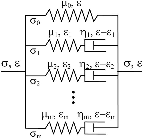
Figure 1 is a schematic diagram of the generalized Maxwell model [3, 21], where a linear spring with the elastic modulus (stiffness constant) μ₀ is connected with m Maxwell elements in parallel. In the i-th Maxwell body, the spring has an elastic modulus μ_i and the dashpot has a viscous coefficient η_i (i = 1, …, m). The stress in the i-th Maxwell body is σ_i = μ_iε_i =η_id(ε−ε_i)/dt.

Fig. 1.

A generalized Maxwell viscoelastic model.

2.1. Differential constitutive equation

Since the components are connected in parallel in Fig. 1, all elements have the same strain (deformation) equal to the overall strain ε(t). The total stress of the whole system is the sum of the stresses in each element, as given by [2, 6]:

$$\sigma \left(t\right)=\sum _{i=0}^m{\sigma }_i\left(t\right)=\left({\mu }_0+\sum _{i=1}^m\frac{D}{D/{\mu }_i+1/{\eta }_i}\right)\varepsilon \left(t\right),$$ (1)

where D = d/dt denotes differentiation with respect to time.

To reduce the number of model parameters, we denote ω_i as the characteristic frequency of i-th Maxwell element and assume that the characteristic frequencies form a geometric series, namely,

$${\omega }_i=\frac{{\mu }_i}{{\eta }_i}={\rho }^{i-1}/\tau (i=1,\dots ,m),$$ (2)

where ρ is a nondimensional real constant characterizing the “gap” between successive frequencies, τ represents the characteristic relaxation time of the first Maxwell element (inverse of the characteristic frequency ω₁).

Substituting Eq. (2) into Eq. (1), we obtain the following differential form of the constitutive equation:

$$\sigma \left(t\right)=\left({\mu }_0+\sum _{i=1}^m\frac{{\mu }_{i}D}{D+{\rho }^{i-1}/\tau }\right)\varepsilon \left(t\right).$$ (3)

The constitutive relation in Eq. (3) still has the main shortcoming of a generalized Maxwell model; i.e., the number of material constants increases with the number of Maxwell elements. Our goal is to acquire a series of μ_i that allows Eq. (3) to capture rate-insensitive hysteresis behavior. To this end, we need to consider the cyclic loading condition.

2.2. Response to oscillatory loading

For convenience, the response of a linear viscoelastic material to an oscillating load is typically studied with complex variable functions [2, 6]. If we assume that the applied load is an oscillatory strain containing a single angular frequency ω (the real part corresponds to the actual load), specifically, the oscillating strain can be written as:

$$\varepsilon \left(t\right)={\varepsilon }_0{e}^{j\omega t},$$ (4)

where ε₀ is the amplitude of strain and $\mathit{\text{j}}=\sqrt{-1}$ denotes the imaginary number. Under the strain loading of Eq. (4), the stress response is also an oscillation at the same frequency with a leading phase angle δ[6]:

$$\sigma \left(t\right)={\sigma }_0{e}^{j\left(\omega t+\delta \right)}=\left({\sigma }_0{e}^{j\delta }\right)e^{j\omega t},$$ (5)

where σ₀ is the amplitude of stress.

According to Eq. (4), the differentiation of strain with respect to time can be simply written as [2, 6]:

$$D\varepsilon \left(t\right)=j\omega \varepsilon \left(t\right),$$ (6)

which reveals that the differentiation D is equivalent to a multiplication by jω.

Bearing in mind Eqs. (4)-(6), the differential constitutive equation (Eq. (3)) can be rewritten as:

$$({\sigma }_0{e}^{j\delta })e^{j\omega t}=\left({\mu }_0+\sum _{i=1}^m\frac{j\omega {\mu }_i}{j\omega +{\rho }^{i-1}/\tau }\right){\varepsilon }_0{e}^{j\omega t}.$$ (7)

From Eq. (7), the complex modulus (or dynamic modulus) [2, 6, 7] of the generalized Maxwell body can be obtained as:

$$E^{\ast }\left(\omega \right)=\frac{\sigma \left(t\right)}{\varepsilon \left(t\right)}=\frac{{\sigma }_0}{{\varepsilon }_0}{e}^{j\delta }={\mu }_0+\sum _{i=1}^m\frac{j\omega {\mu }_i}{j\omega +{\rho }^{i-1}/\tau }.$$ (8)

The mechanical loss (a measure of the internal friction) is defined as the tangent of the phase angle δ[2, 6, 7]:

$$\text{tan}\left(\delta \right)=\frac{\text{Im}\left(E^{\ast }\left(\omega \right)\right)}{\text{Re}\left(E^{\ast }\left(\omega \right)\right)},$$ (9)

where Re and Im represent the real and imaginary parts of the complex variable, respectively. The nondimensional tan(δ) in Eq. (9) is a function of frequency ω and is proportional to the ratio of dissipated energy to stored energy in a dynamic loading cycle [7]. Thus rate insensitivity of the generalized Maxwell model can be realized by selecting an appropriate elastic modulus for each Maxwell element to make tan(δ) nearly independent of ω. We found that the following series of elastic moduli fits the criterion:

$${\mu }_i=\beta {\left(1+\beta \right)}^{i-1}{\mu }_0(i=1,\dots ,m),$$ (10)

where β= μ₁/μ₀ is the ratio of the elastic modulus of the first Maxwell body (which has a characteristic relaxation time τ as shown in Eq. (2)) to that of the first spring (see Fig. 1). Using Eq. (10), the differential constitutive model (Eq. (3)) can be written as:

$$\sigma \left(t\right)={\mu }_0\left(1+\beta \sum _{i=1}^m\frac{{\left(1+\beta \right)}^{i-1}D}{D+{\rho }^{i-1}/\tau }\right)\varepsilon \left(t\right),$$ (11)

and the complex modulus (Eq. (8)) becomes:

$$E^{\ast }\left(\omega \right)={\mu }_0\left(1+\beta \sum _{i=1}^m\frac{j\omega {\left(1+\beta \right)}^{i-1}}{j\omega +{\rho }^{i-1}/\tau }\right).$$ (12)

There are five material constants in the model: μ₀, τ, m, ρ and β, where μ₀ has the unit of stress, τ has the unit of time, and the other three parameters are nondimensional. For given model parameters, the internal friction [2] or the normalized energy dissipation [3] can be examined by plotting tan(δ) against frequency ω (the normalized energy dissipation differs from tan(δ) by a multiplication factor [7]).

The real part of the applied complex strain load in Eq. (4) is a cosine function containing a single angular frequency ω:

$$\varepsilon \left(t\right)={\varepsilon }_0\text{cos}\left(\omega t\right).$$ (13)

The corresponding stress response is the real part of Eq. (5), which is another cosine function with the same frequency [6, 7]:

$$\sigma \left(t\right)={\sigma }_0\text{cos}\left(\omega t+\delta \right).$$ (14)

The hysteresis loop can be obtained by plotting σ(t) versus ε(t), which should be nearly independent of angular frequency ω in a wide range, because the internal friction tan(δ) is insensitive to the loading frequency.

2.3. Relaxation and creep functions

Under a given constant strain load ε₀, the relaxation function can be expressed by [2, 6, 7]:

$$G\left(t\right)=\frac{\sigma \left(t\right)}{{\varepsilon }_0}={\mu }_0+\sum _{i=1}^m{\mu }_i{e}^{-{\omega }_{i}t}.$$ (15)

Using Eqs. (2) and (10), the reduced relaxation function [2] can be obtained from Eq. (15) as:

$$g\left(t\right)=\frac{G\left(t\right)}{G\left(0\right)}=\frac{1+\beta \sum _{i=1}^m{\left(1+\beta \right)}^{i-1}{e}^{-{\rho }^{i-1}t/\tau }}{1+\beta \sum _{i=1}^m{\left(1+\beta \right)}^{i-1}},$$ (16)

from which one can easily show that

$$g\left(0\right)=1,g(\infty )=\frac{1}{{\left(1+\beta \right)}^m}.$$ (17)

Equation (17) indicates that the lower bound of the reduced relaxation function, g(∞), depends on m and β only.

Under a constant stress load σ₀, the strain of a viscoelastic body varies with time. The creep function (compliance) of a linear viscoelastic material can be defined by [2, 6, 7]:

$$J\left(t\right)=\frac{\varepsilon \left(t\right)}{{\sigma }_0}.$$ (18)

According to the linear viscoelastic theory, the creep function and the relaxation function are related by the following convolution [6, 7]:

$${\int }_0^{t}J\left(t-\xi \right)E\left(\xi \right)d\xi =t.$$ (19)

Equation (19) can be used to obtain the creep function if the relaxation function is known, or vice versa. Findley et al. [6] provided a partial fraction expansion method to solve Eq. (19) using Laplace transform.

In the following section, we will demonstrate numerically that the rate insensitive behavior can be predicted by choosing appropriate model parameters, especially m and ρ; i.e., the number of Maxwell bodies and the gap between characteristic frequencies.

2.4. Numerical examples

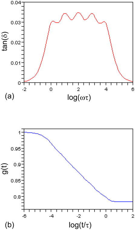
The internal friction, tan(δ), depends on only four parameters: τ, m, ρ and β (Eqs. (9) and (12)), so does the reduced relaxation function g(t) (Eq. (16)). To compare them with the results in Holzapfel et al. [3] where 5 Maxwell bodies were used, we chose τ = 1.0 s, m = 5, ρ = 10.0, β = 0.05. Figure 2(a) shows that tan(δ) is nearly constant within four decades of time (0 < log(ωτ) < 4), similar to the dissipation energy plot in [3]. Figure 2(b) reveals that g(t) decreases from 1.0 to 0.78 after four decades (-4 < log(t/τ) < 0), consistent with the result in [3].

Fig. 2.

(a) The internal friction tan(δ) versus log(ωτ). (b) The reduced relaxation function g(t) versus log(t/τ). τ= 1.0 s, m = 5, ρ = 10.0, β= 0.05.

Ten material constants are required for the model in Holzapfel et al. [3]. The number of parameters in our model is five and it does not depend on how many Maxwell bodies are employed. Thus we can easily increase m to cover a larger rate insensitive range and decrease ρ to remove the ripples in Fig. 2(a), without changing the number of material constants.

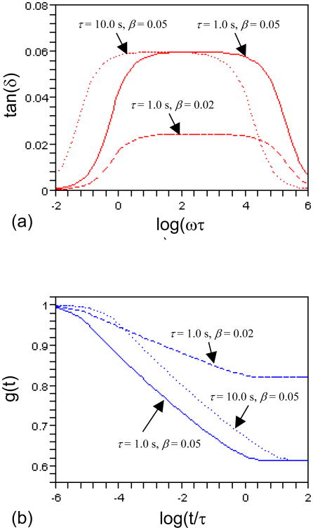
In Fig. 3, we chose ten Maxwell elements with m = 10 and ρ = 3.6. Figure 3(a) demonstrates that tan(δ) can be smoothened with a larger m and a smaller ρ (compare the solid curve in Fig. 3(a) with Fig. 2(a)). Figures 3(a) and (b) illustrate, respectively, that a decrease in β means smaller mechanical loss and less stress relaxation, if we compare the solid (β= 0.05) and the dashed (β= 0.02) plots. The dependence of g(t) on m is reflected by the minima of the solid curves in Figs. 2(b) and 3(b). By comparing the solid (τ= 1.0 s) and the dotted (τ= 10.0 s) curves in Fig. 3, one can see that tan(δ) and g(t) maintain their shapes but shift with τ on the ω and t axes, indicating that τ can be used to locate the rate insensitive range on the frequency or time axes (also see Eqs. (9), (12) and (16)).

Fig. 3.

The plots of (a) tan(δ) versus log(ωτ₀) and (b) g(t) versus log(t/τ₀). m = 10, ρ = 3.6. Note that τ₀ = 1.0 sec. has been used to avoid awkward units in abscissas.

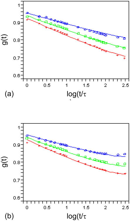
To demonstrate how the model parameters can be adjusted to fit the experimental data, we compare g(t) with some reduced relaxation functions reported by Tanaka and Fung [1]. The experimental results of canine aortic arch and proximal thoracic artery were plotted in Figs. 4(a) and (b) as three set of symbols, respectively. For brevity, we fixed ρ as 3.6 in all cases. Then parameters m, τ, and β were varied to obtain a good match of the model prediction and experimental data. It is noted that a rigorous fit was not performed here. The purpose of this example is to show how model parameters can be generally varied to fit the data. In the case of aortic arch (Fig. 4(a)), it was found that m = 6 and τ= 400.0 s can be selected, and β= 0.038, 0.052, and 0.065 can be used to represent the three set of data very well. In the case of proximal thoracic artery (Fig. 4(b)), the selection of m = 5, τ= 120.0 s, β= 0.038, 0.052, and 0.065 is sufficient to capture the experimental results.

Fig. 4.

The reduced relaxation function g(t) of the linear model (curves) compared with experimental data (symbols) in [1]. (a) m = 6 and τ= 400.0 s fitted to canine aortic arch. (b) m = 5 and τ= 120.0 s fitted to canine proximal thoracic artery. β= 0.038, 0.052, 0.065 from top to bottom. ρ= 3.6 and τ₀ = 1.0 sec.

It should be cautioned that the above comparison was based on relaxation curves only. Hence, the selected model parameters can not necessarily capture other hysteresis features (e.g., the internal friction). If more experimental results (such as the width and magnitude of the internal friction plot in Fig. 3(a)) are known, the best set of model parameters can be obtained using a least square method. Then both the stress relaxation and the hysteresis loop can be appropriately predicted by the model.

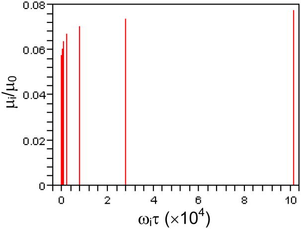
Since the amplitude μ_i(ω_i) in Eq. (15) is a spectrum of the relaxation function on the frequency axis ω_i [2], we can plot the μ_i in Eq. (10) against the ω_i in Eq. (2) to illustrate how the elastic modulus changes with the characteristic frequency. Figure 5 shows the plot of μ_i/μ₀ versus ω_iτ for ρ= 3.6, β= 0.05, and i = 1, …, 10 (corresponding to the solid curves in Fig. 3). It is seen that amplitude of the discrete spectrum increases nonlinearly with frequency, which is important for the model to be rate independent in a multiple time scale, as shown in Fig. 3(a).

Fig. 5.

A plot of μ_iμ₀ versus ω_iτ(i.e., β(1+β)^i-1 vs. ρ^i-1), the normalized discrete spectrum of the relaxation function, for ρ= 3.6, β= 0.05, and i = 1, 2, …, 10.

If we consider a simpler series of elastic moduli; e.g., constant amplitude μ_i = βμ₀ for all the Maxwell bodies (i = 1, …, m), then the complex modulus (Eq. (8)) becomes

$$E^{\ast }\left(\omega \right)={\mu }_0\left(1+\beta \sum _{i=1}^m\frac{j\omega }{j\omega +{\rho }^{i-1}/\tau }\right).$$ (20)

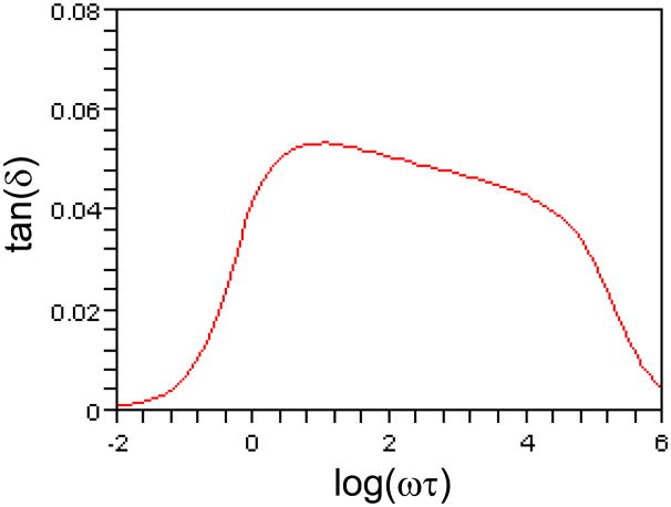
The internal friction tan(δ) versus log(ωτ) plot, computed by Eqs. (9) and (20), is shown in Fig. 6, where the same parameters for the solid curve in Fig. 3(a) have been used. It is seen that constant amplitude for the relaxation function (μ_i = βμ₀) does not result in rate insensitive mechanical loss tan(δ), implying that the choice of Eq. (10) is essential in this model.

Fig. 6.

A plot of tan(δ) versus log(ωτ) when constant amplitude of the relaxation function (μ_i = βμ₀) is considered. τ= 1.0 s, m = 10, ρ= 3.6, β= 0.05.

3. Discussion

Since the viscoelastic hysteresis loop in a discrete spectrum system is maximized when the loading frequency matches the characteristic relaxation frequency [2], generalized Maxwell models with different relaxation constants should be considered to account for the rate insensitive viscoelasticity of biomaterials [3].

We have shown that the number of parameters in a generalized Maxwell model can be significantly decreased by considering a geometric series of the characteristic frequencies of Maxwell bodies (Eq. (2)). A similar series for elastic moduli of the springs has been exploited to reduce the number of material constants (Eq. (10)). In this section, we will consider some of the issues related to the proposed linear viscoelastic model.

3.1. Model parameters

The physical meanings of the five parameters in our model are as follows: μ₀ is the relaxed elastic modulus when time approaches infinity (i.e., all dashpots are fully relaxed and the viscous stress becomes zero); τ is the characteristic relaxation time that positions the rate-insensitive range; m denotes the number of spring-dashpot elements; ρ reflects the gap between consecutive characteristic frequencies; β is equal to the ratio of elastic modulus of the Maxwell body with characteristic relaxation time τ to that of the pure spring. It should be noted that the initial elastic modulus at t = 0 (instant elastic modulus) can be derived from Eqs. (15)-(17) as μ₀(1+β)^m.

Iatridis et al. [20] utilized a 5-parameter generalized Maxwell model with only two spring-dashpot elements and noted that the ratio of viscous coefficients to relaxation times (i.e., the amplitude of relaxation spectrum) is nearly constant. Their study implied that the number of parameters can be reduced when more Maxwell elements are used. The relaxation times chosen by Holzapfel et al. [3] in their model actually form a geometric series with ρ = 10, indicating that the characteristic frequencies are related by harmony. The novelty of our model is that relations between parameters have been explicitly considered (see Eqs. (2) and (10)). In the discrete spectrum approximation of quasi-linear viscoelastic theory developed by Puso and Weiss [22], a formula similar to Eq. (16) has been used to estimate the exponential integral relaxation function with a continuous spectrum [15].

3.2. Microstructural basis for the multi-element model and parameter method

It is well known that the microstructure of biological tissues is not random but follows certain patterns. Also, the mechanical properties of biological tissues are related to microstructure. For example, the Young's modulus of the intima-media layer of arteries, which consists of endothelial and smooth muscle cells along with elastic lamina, was found to be several times larger than that of the adventitia layer at relatively small or physiological loading conditions [23, 24]. The latter is composed of collagen with a small amount of fibroblasts and elastin.

From a microstructural point of view, specific orientation relations exist between the collagen fibers in arteries [3] and between the myocardial fibers in hearts [25]; i.e., a linear relation of fiber angle versus transmural depth [26]. These intrinsic geometrical and mechanical variations are undoubtedly reflected in the macroscopic behavior of the biological materials.

Soft tissue is essentially a fiber in a matrix composite. In the generalized Maxwell model, the fibers are analogous to springs, and matrix to dashpots. The collagen fiber coils stretch and store energy similar to springs and the cellular matrix provides damping similar to the dashpot.

Based on the relationship between material properties and microstructural constitution along spatial depth [23, 24, 26], a biological tissue can be regarded as a finite number of pseudo-layers, each with a finite thickness. In the present model, each of these pseudo-layers is in effect represented by a spring-dashpot element. The more pseudo-layers, the more elements, and the smoother the response curve. This is analogous to the case where we mathematically lump a continuous spectrum into a discrete spectrum; i.e., employ a generalized Maxwell model to approximate the real continuous media.

Taking into consideration that the material constitution and mechanical properties vary from layer to layer (although there are relations or patterns partially due to the connections between adjacent layers), we propose that particular relations exist between the Maxwell bodies as shown in Eqs. (2) and (10). It should be emphasized that the order of the Maxwell elements in Fig. 1 is not necessarily the same as the order of the layers in the tissue. In other words, the mechanical properties (i.e., ω_i in Eq. (2) and μ_i in Eq. (10)) in the model can be mathematically simulated by a simple series.

The experimentally measured mechanical properties of dissected layers can help define model parameters such as ρ and β (Eqs. (2) and (10)). The fundamental advantage of this model is that the number of material constants stays the same even if the number of elements increases dramatically. This is due to the proportional relationship between the model parameters (the connection between elementary layers). Therefore, in specific applications (e.g., mechanics of arteries or myocardium), the relations between the parameters for the layers at various depths in the model can be tuned according to the experimental data.

The above reasoning provides a physical basis for the proposed multi-element model. It also offers a biological microstructural basis for the parameterization method proposed in this study. These methods could be applied to a wide range of biological soft tissue types. Nevertheless, the concept of finite pseudo-layers may not be applicable to all biological tissues, such as the heel pad.

3.3. Model advantage and limitation

The one-dimensional model (Eqs. (11) and (16)) can be used to analyze the viscoelastic behavior of biomaterials under uniaxial tension or other simple loadings. It is simple to extend the linear viscoelastic model to three-dimensions using tensor notation [2, 6, 7]. Finite element implementation of the model can be done following well established approaches [3, 12, 15, 16, 21].

The proposed model is intended for rate insensitive linear viscoelastic materials (note that nonlinear stress-strain relationships can be linearized with an alternative strain measure), especially for biological soft tissues with hysteresis curves nearly independent of loading frequency. It has been noted that some biological materials are rate sensitive [12, 16, 27, 28], to which this model may not apply. However, the notion of harmonic (or a series of) frequencies may still be useful to reduce model parameters. For example, Fig. 6 shows a rate sensitive linear viscoelastic model.

One limitation of the current model is the high-order differential equation (Eq. (11)), which is not convenient to use in numerical simulations. Fortunately, the concept of internal variables can be exploited to incorporate the model in numerical methods [3, 7, 12]. Nevertheless, it will be interesting to determine how to coordinate the evolution equations of the internal variables since the parameters of Maxwell bodies are related. As our model can be viewed as a discrete form of the quasi-linear viscoelastic formulation, it can be expected that some viscoelastic behaviors such as creep may not be captured very well [2].

The main advantage of this model is that it requires only five material constants regardless of the number of Maxwell bodies used. The rate insensitive frequency range is controlled by parameters m and ρ; i.e., the number of the Maxwell elements and the gap between characteristic frequencies. For m = 5, our model represents a special case of the five-element model in Ref. [3], m = 2 results in a model similar to those in Refs. [17, 20], and m = 1 corresponds to the standard linear solid that has been widely used for its simplicity [2, 7, 29-31]. Equivalent forms of models; e.g., a linear spring connected in series with a number of Voigt bodies [2, 6, 21, 29, 32], can be formulated in a similar manner.

4. Conclusions

We propose a generalized Maxwell model that captures the rate insensitive hysteresis behavior of linear viscoelastic biomaterials. By considering a geometric series of characteristic frequencies and the relation between elastic moduli of the springs, the model is characterized by only five material constants that have some physical meanings. As a result, the parameter determination process can be simplified; e.g., the relaxation function can be fitted with experimental data. It is expected that the present model is applicable to other engineering materials where rate insensitive viscoelastic behaviors are found (e.g., see review in [2]) as well as typical biological soft tissues.

References

- 1.Tanaka TT, Fung YC. Elastic and inelastic properties of the canine aorta and their variations along the aortic tree. J Biomech. 1974;7:357–70. doi: 10.1016/0021-9290(74)90031-1. [DOI] [PubMed] [Google Scholar]
- 2.Fung YC. Biomechanics: mechanical properties of living tissues. second. New York: Springer; 1993. [Google Scholar]
- 3.Holzapfel GA, Gasser TC, Stadler M. A structural model for the viscoelastic behavior of arterial walls: continuum formulation and finite element analysis. Eur J Mech A-Solids. 2002;21:441–63. [Google Scholar]
- 4.Weiss JA, Gardiner JC, Bonifasi-Lista C. Ligament material behavior is nonlinear, viscoelastic and rate-independent under shear loading. J Biomech. 2002;35:943–50. doi: 10.1016/s0021-9290(02)00041-6. [DOI] [PubMed] [Google Scholar]
- 5.Grashow JS, Yoganathan AP, Sacks MS. Biaixal stress-stretch behavior of the mitral valve anterior leaflet at physiologic strain rates. Ann Biomed Eng. 2006;34:315–25. doi: 10.1007/s10439-005-9027-y. [DOI] [PubMed] [Google Scholar]
- 6.Findley WN, Lai JS, Onaran K. Creep and relaxation of nonlinear viscoelastic materials. New York: Dover; 1989. [Google Scholar]
- 7.Lakes RS. Viscoelastic solids. Boca Raton: CRC Press; 1999. [Google Scholar]
- 8.Pioletti DP, Rakotomanana LR. Non-linear viscoelastic laws for soft biological tissues. Eur J Mech A-Solids. 2000;19:749–59. [Google Scholar]
- 9.Rubin MB, Bodner SR. A three-dimensional nonlinear model for dissipative response of soft tissue. Int J Solids Struct. 2002;39:5081–99. [Google Scholar]
- 10.Humphrey JD. Continuum biomechanics of soft biological tissues. Proc R Soc London A. 2003;459:3–46. [Google Scholar]
- 11.Vito RP, Dixon SA. Blood vessel constitutive models-1995-2002. Annu Rev Biomed Eng. 2003;5:413–39. doi: 10.1146/annurev.bioeng.5.011303.120719. [DOI] [PubMed] [Google Scholar]
- 12.Haslach HW. Nonlinear viscoelastic, thermodynamically consistent, models for biological soft tissue. Biomechan Model Mechanobiol. 2005;3:172–89. doi: 10.1007/s10237-004-0055-6. [DOI] [PubMed] [Google Scholar]
- 13.Funk JR, Hall GW, Crandall JR, Pilkey WD. Linear and quasi-linear viscoelastic characterization of ankle ligaments. J Biomech Eng. 2000;122:15–22. doi: 10.1115/1.429623. [DOI] [PubMed] [Google Scholar]
- 14.Sverdlik A, Lanir Y. Time-dependent mechanical behavior of sheep digital tendons, including the effects of preconditioning. J Biomech Eng. 2002;124:78–84. doi: 10.1115/1.1427699. [DOI] [PubMed] [Google Scholar]
- 15.Bischoff JE. Reduced parameter formulation for incorporating fiber level viscoelasticity into tissue level biomechanical models. Ann Biomed Eng. 2006;34:1164–72. doi: 10.1007/s10439-006-9124-6. [DOI] [PubMed] [Google Scholar]
- 16.Vena P, Gastaidi D, Contro R. A constituent-based model for the nonlinear viscoelastic behavior of ligaments. J Biomech Eng. 2006;128:449–57. doi: 10.1115/1.2187046. [DOI] [PubMed] [Google Scholar]
- 17.Wu XY, Levenston ME, Chaikof EL. A constitutive model for protein-based materials. Biomaterials. 2006;27:5315–25. doi: 10.1016/j.biomaterials.2006.06.003. [DOI] [PubMed] [Google Scholar]
- 18.Zhang W, Kassab GS. A bilinear stress–strain relationship for arteries. Biomaterials. 2007;28:1307–15. doi: 10.1016/j.biomaterials.2006.10.022. [DOI] [PMC free article] [PubMed] [Google Scholar]
- 19.Iatridis JC, Kumar S, Foster RJ, Weidenbaum M, Mow VC. Shear mechanical properties of human lumbar annulus fibrosus. J Orthop Res. 1999;17:732–7. doi: 10.1002/jor.1100170517. [DOI] [PubMed] [Google Scholar]
- 20.Iatridis JC, Wu JR, Yandow JA, Langevin HM. Subcutaneous tissue mechanical behavior is linear and viscoelastic under uniaxial tension. Connect Tissue Res. 2003;44:208–17. [PubMed] [Google Scholar]
- 21.Idesman A, Niekamp R, Stein E. Finite elements in space and time for generalized viscoelastic Maxwell model. Comput Mech. 2001;27:49–60. [Google Scholar]
- 22.Puso MA, Weiss JA. Finite element implementation of anisotropic quasi-linear viscoelasticity using a discrete spectrum approximation. J Biomech Eng. 1998;120:62–70. doi: 10.1115/1.2834308. [DOI] [PubMed] [Google Scholar]
- 23.Yu QL, Zhou JB, Fung YC. Neutral axis location in bending and youngs modulus of different layers of arterial-wall. Am J Physiol Heart Circ Physiol. 1993;265:H52–60. doi: 10.1152/ajpheart.1993.265.1.H52. [DOI] [PubMed] [Google Scholar]
- 24.Xie JP, Zhou JB, Fung YC. Bending of blood-vessel wall - stress-strain laws of the intima-media and adventitial layers. J Biomech Eng. 1995;117:136–45. doi: 10.1115/1.2792261. [DOI] [PubMed] [Google Scholar]
- 25.Streeter DD, Spotnitz HM, Patel DP, Ross J, Sonnenblick EH. Fiber orientation in the canine left ventricle during diastole and systole. Circ Res. 1969;24:339–47. doi: 10.1161/01.res.24.3.339. [DOI] [PubMed] [Google Scholar]
- 26.Chen JJ, Song SK, Liu W, McLean M, Allen JS, Tan J, Wickline SA, Yu X. Remodeling of cardiac fiber structure after infarction in rats quantified with diffusion tensor MRI. Am J Physiol Heart Circ Physiol. 2003;285:H946–54. doi: 10.1152/ajpheart.00889.2002. [DOI] [PubMed] [Google Scholar]
- 27.Gamero LG, Armentano RL, Barra JG, Simon A, Levenson J. Identification of arterial wall dynamics in conscious dogs. Exp Physiol. 2001;86:519–28. doi: 10.1113/eph8602172. [DOI] [PubMed] [Google Scholar]
- 28.Kiss MZ, Varghese T, Hall TJ. Viscoelastic characterization of in vitro canine tissue. Phys Med Biol. 2004;49:4207–18. doi: 10.1088/0031-9155/49/18/002. [DOI] [PMC free article] [PubMed] [Google Scholar]
- 29.Orosz M, Molnarka G, Monos E. Curve fitting methods and mechanical models for identification of viscoelastic parameters of vascular wall - a comparative study. Med Sci Monit. 1997;3:599–604. [Google Scholar]
- 30.Veress AI, Vince DG, Anderson PM, Cornhill JF, Herderick EE, Kuban BD, Greenberg NL, Thomas JD. Vascular mechanics of the coronary artery. Z Kardiol. 2000;89:92–100. doi: 10.1007/s003920070106. [DOI] [PubMed] [Google Scholar]
- 31.Rehal D, Guo XM, Lu X, Kassab GS. Duration of no-load state affects opening angle of porcine coronary arteries. Am J Physiol Heart Circ Physiol. 2006;290:H1871–8. doi: 10.1152/ajpheart.00910.2005. [DOI] [PubMed] [Google Scholar]
- 32.Berglund JD, Nerem RM, Sambanis A. Viscoelastic testing methodologies for tissue engineered blood vessels. J Biomech Eng. 2005;127:1176–84. doi: 10.1115/1.2073487. [DOI] [PubMed] [Google Scholar]