Longitudinally guided level sets for consistent tissue segmentation of neonates

Abstract

Quantification of brain development as well as disease‐induced pathologies in neonates often requires precise delineation of white matter, grey matter and cerebrospinal fluid. Unlike adults, tissue segmentation in neonates is significantly more challenging due to the inherently lower tissue contrast. Most existing methods take a voxel‐based approach and are limited to working with images from a single time‐point, even though longitudinal scans are available. We take a different approach by taking advantage of the fact that the pattern of the major sulci and gyri are already present in the neonates and generally preserved but fine‐tuned during brain development. That is, the segmentation of late‐time‐point image can be used to guide the segmentation of neonatal image. Accordingly, we propose a novel longitudinally guided level‐sets method for consistent neonatal image segmentation by combining local intensity information, atlas spatial prior, cortical thickness constraint, and longitudinal information into a variational framework. The minimization of the proposed energy functional is strictly derived from a variational principle. Validation performed on both simulated and in vivo neonatal brain images shows promising results. Hum Brain Mapp, 2013. © 2011 Wiley Periodicals, Inc.

INTRODUCTION

Longitudinal MRI study involving neonates provides a unique opportunity for studying early brain development patterns. Quite a number of sets of longitudinal data have been acquired and analyzed in various institutes [Almlia et al., 2007; Dubois et al., 2008; Gerig et al., 2006; Knickmeyer et al., 2008]. Accurate segmentation of neonatal magnetic resonance (MR) images plays an indispensible role in the brain development studies involving full‐term and preterm infants, as well as infants at high risks for neurodevelopmental disorders, such as autism and schizophrenia. Despite the success of segmentation methods developed for adult brains [Awate et al., 2006; Guillemaud and Brady, 1997; Leemput et al., 1999; Wells et al., 1996], segmentation of neonatal brain images remains challenging, due mainly to the insufficient spatial resolution, low image contrast, and ambiguous tissue intensity distribution.

To obtain more reliable segmentation results, atlas‐based segmentation methods are widely used [Cocosco et al., 2003; Prastawa et al., 2005; Song et al., 2007; Warfield et al., 2000; Weisenfeld and Warfield 2009]. An atlas can be generated from manual/automatic segmentation results of an individual image, or a group of images from different individuals [Kuklisova‐Murgasova et al., 2010; Shi et al., 2010]. For example, Prastawa et al. [Prastawa et al., 2005; Weisenfeld et al., 2006] proposed an atlas‐based approach for neonatal brain segmentation. They generated an atlas by averaging three semiautomatically segmented neonatal brain images and adopted the expectation‐maximization (EM) scheme with inhomogeneity correction for tissue classification. Bhatia et al. [ 2004] produced an unbiased average atlas by group‐wise registration of all images in the population. Warfield et al. [ 2000] proposed an age‐specific atlas that is generated from multiple subjects using an iterative tissue‐segmentation‐and‐atlas‐alignment strategy to improve neonatal tissue segmentation. However, one common limitation of average‐shape atlases is that subtle brain structures, especially those in the cortical regions, are usually diminished in the process of atlas construction, due to intersubject anatomical variability and registration error. As proposed in [Aljabar et al., 2009; Shi et al., 2010], an atlas generated from images that are similar to the to‐be‐segmented image, e.g., longitudinal data, produces more accurate segmentation results than atlases generated from randomly selected images. Shi et al. [ 2010] proposed a novel approach for neonatal brain segmentation by utilizing an atlas built from the longitudinal follow‐up of the same subject (i.e., the image scanned at the one‐year or two‐year old) to guide neonatal image segmentation.

We note, however, that the above‐mentioned methods are voxel‐based approaches, which cannot guarantee smooth and closed segmentation contours/surfaces. To this end, level sets [1988] are widely used [Cremers et al., 2007; Gooya et al., 2008; Li et al., 2008a; Li et al., 2009; Rousson and Cremers 2005; Yezzi et al., 2000]. Many level‐set‐based algorithms have been proposed for brain image segmentation [Goldenberg et al., 2002; Han et al., 2004; MacDonald et al., 2000; Xu et al., 1999; Zeng et al., 1999]. On the basis of the fact that the cortex has a nearly constant thickness, Zeng et al. [ 1999] first introduced the idea of coupled level sets for segmentation of the brain cortex. The ideas introduced by Zeng et al. were extended by Goldenberg et al. who proposed a fast variational geometric approach for cortex segmentation [Goldenberg et al., 2002]. Despite the success of these level‐sets based methods in adult brain images, few works focus on the segmentation of brain images of neonates. Xue et al. [ 2007] proposed an EM‐MRF segmentation scheme for tissue classification and partial volume (PV) correction. The cortical surfaces for neonates were then reconstructed using implicit surface evolution. However, this method is prone to systematic misclassifications due to overlaps of tissue distributions of WM and GM classes [Kuklisova‐Murgasova et al., 2010].

Also, most existing neonatal segmentation methods do not make full use of longitudinal information and are limited to single‐time‐point images even though longitudinal scans are available. In this article, we propose a novel longitudinally guided level‐sets for consistent tissue segmentation of neonatal images. Our model is based on the fact that at term birth, the major sulci and gyri are already present in the neonates [Chi et al., 1977]. The pattern of the major sulci and gyri are generally preserved but are fine‐tuned during brain development [Armstrong et al., 1995]. Specifically, the cortical convolutions emerge in the late gestation before birth [Hill et al., 2010], with extensive folding occurs during the third trimester [Abe et al., 2003; Dubois et al., 2008]. At term birth, although the brain is only one‐third of adult volume [Lebel et al., 2008; Thompson et al., 2007], the major sulci and gyri present in the adult are already established [Chi et al., 1977]. Therefore, we can utilize the longitudinal segmentation result from the late‐time‐point image, which can be achieved with high accuracy by the existing segmentation methods, to guide the segmentation of neonatal image.

Specifically, we first use the adaptive fuzzy c‐means algorithm [Pham and Prince, 1999] and the coupled level sets [Wang et al., 2011] to segment late‐time‐point image (Year2) and neonatal image (Year0) independently. We then warp the segmentation result of Year2 to the Year0 space using deformable registration [Shen and Davatzikos, 2002] to guide Year0 image segmentation. The proposed method is based on our previous work [Wang et al., 2011], but with important differences. First, the current method utilizes the longitudinal information, which enables it to achieve accurate and consistent segmentation results across time points. Second, a closed‐form solution to the minimization problem of the proposed energy is provided. Note that although the detection of myelination and maturation of WM is also very important in early development study [Prastawa et al., 2005; Weisenfeld and Warfield, 2009], this paper focuses on segmentation of brain into general GM, WM, and CSF, in which WM contains both myelinated and unmyelinated WM, and GM contains both cortical and subcortical GM.

METHOD

The proposed framework, summarized in Figure 1, consists of three steps: (1) fuzzy segmentation of the late‐time‐point image, and construction of its cortical surfaces (WM/GM surface and GM/CSF surface), (2) robust segmentation of neonatal image based on convex optimization and coupled level sets, and (3) warping of the surfaces of late‐time‐point image to the neonatal image space and then longitudinally guide the level sets for improved neonatal image segmentation.

Figure 1.

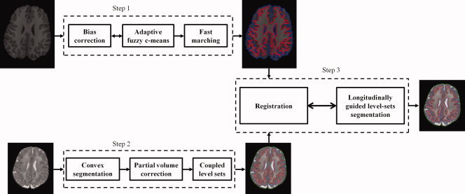
The proposed framework for consistent segmentation of neonatal images. [Color figure can be viewed in the online issue, which is available at wileyonlinelibrary.com.]

Fuzzy Segmentation of the Late‐Time‐Point Image and Reconstruction of Its Cortical Surfaces

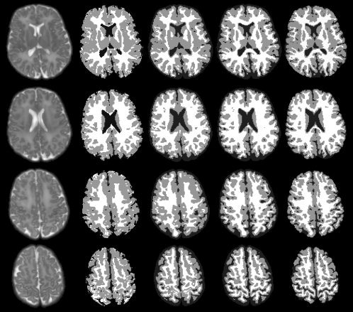
To robustly segment late‐time‐point image, we adopt a well‐established automatic brain tissue segmentation method, namely the adaptive fuzzy c‐means (AFCM) algorithm [Pham and Prince, 1999], which integrates both bias correction and tissue classification into a single framework. The AFCM algorithm is an extension of the standard FCM algorithm. For a given image I, AFCM seeks to determine the memberships u _x,k, centroids v _k, and gain field g,

(1)

 The value u _x,k is the membership of the pixel at location x with respect to class k such that ∑${}_{\mathit{\text{k}}\text{= 1}}^{\mathit{\text{C}}}$ u _x,k = 1. The parameter q is a weighting exponent on each fuzzy membership and determines the degree of fuzziness for classification. The parameter q is usually set as 2 in many applications [Pham and Prince, 1999]. The last two terms are regularization terms to ensure that g is spatially smooth and slow varying, and D _r and D _s are the finite difference operators along the r‐th and the s‐th dimension of the image, respectively. This energy can be minimized by iteratively updating the membership functions, centroids, and gain field.

In this paper, we employ the images of the two‐year‐olds (Year2) to guide segmentation of the images of neonates. Typical AFCM image segmentation results of a two‐year‐old are shown in Figure 2. On the basis of the segmentation results given by AFCM, we can construct the WM/GM surface and GM/CSF surface using fast marching [Sethian, 1999]. We denote the reconstructed zero‐level surfaces, representing the WM/GM and GM/CSF boundaries, as and , respectively.

Figure 2.

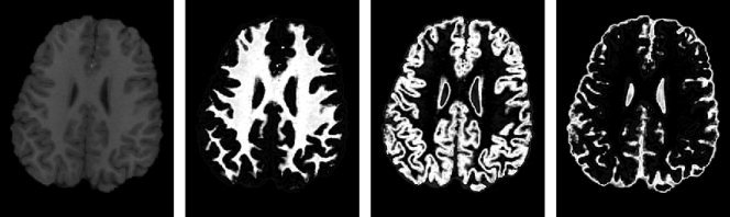
Fuzzy segmentation of the brain image of a two‐year‐old. From left to right: the original image, segmented WM, GM and CSF.

Initial Neonatal Image Segmentation Using Coupled Level Sets

We adopt our previous algorithm [Wang et al., 2011], a coupled level‐sets method, for initial segmentation of the neonatal images. For completeness, the method is summarized in the following.

The coupled level‐sets method combines local intensity information [Wang et al., 2009], atlas spatial prior information prior_i, and cortical thickness constraint into a single level‐set‐based framework. As illustrated in the left panel of Figure 3, by using Heaviside function H, three level‐set functions1 ϕ₁, ϕ₂, and ϕ₃ were used to define regions M ₁ = H (ϕ₁) H (ϕ₂)H (ϕ₃), M ₂ = (1 − H (ϕ₁)) H (ϕ₂)H (ϕ₃), M ₃ = (1 − H (ϕ₂)) H (ϕ₃) and M ₄ = 1 − H (ϕ₃) to represent the WM, GM, CSF and background, respectively. The energy using local Gaussian distribution fitting and population‐atlas prior prior_i was first defined as follows,

(2)

where x (or y) denotes a voxel location of image I, ϕ = (ϕ₁, ϕ₂, ϕ₃), and ω_σ is a Gaussian kernel with scale σ for controlling the size of the local region [Li 2006; Li et al., 2007; Li et al., 2008b]. The spatial prior prior_i is a neonatal atlas2 generated from 95 neonatal subjects, as described in [Shi et al., 2011]. We used the HAMMER algorithm [Shen and Davatzikos, 2002] to warp this atlas to the subject image space. p_i,x (I(y)) is the Gaussian probability density with spatially varying means u _i (x) and variances σ${}_{\mathit{\text{i}}}^{\text{2}}$ (x), defined as , and L(ϕ_j) = ∫| ∇ H (ϕ_j (x))|dx is the length term to maintain surface smoothness during evolution. The gradient descent flow equations to minimize the energy functional E _{L_prior} (2) in can be derived by calculus of variation. Since cortical thickness does not vary dramatically, a cortical thickness constraint term was defined and added to the gradient descent flow equations. Let the allowed distance be [d D], with d (D) be the minimal (maximal) allowed distance between the outer and inner cortical surfaces. The cortical thickness constraint term will deflate (inflate) the inner (outer) surface if the distance is below the minimum acceptable value d, and inflate (deflate) the inner (outer) surface if the distance is beyond the maximum acceptable value D.

Figure 3.

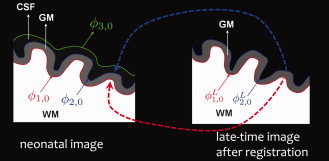
Longitudinally guided level‐set segmentation. The evolution of and is constrained by longitudinal information. and are the zero‐level‐sets of and , respectively. [Color figure can be viewed in the online issue, which is available at wileyonlinelibrary.com.]

We have shown in [Wang et al., 2011] that this framework is capable of achieving reasonable segmentation results for neonatal brain images. It is, however, currently limited to working with images from a single time‐point, even though longitudinal scans are available. In addition, the cortical thickness constraint terms are artificially incorporated into the gradient descent flow equations, and are not strictly derived from a minimization problem. In the following, we will propose a novel longitudinally guided level‐sets strategy for consistent neonatal image segmentation.

Longitudinally Guided Level‐Sets Method For Segmentation of Neonatal Brain Images

To effectively utilize the late‐time‐point image information for guiding neonatal image segmentation, we first register, using HAMMER [Shen and Davatzikos, 2002], the segmentation image of the two‐year‐old obtained in step 1 (Fig. 1) to the respective neonatal image. Using the estimated deformation field, and are warped similarly, resulting in ϕ${}_{\text{1}}^{\text{L}}$ and ϕ${}_{\text{2}}^{\text{L}}$ respectively. On the basis of the observation that the pattern of the major sulci and gyri are generally preserved but are fine‐tuned during brain development, the distance between the zero‐level‐surfaces of ϕ₁ (or ϕ₂) and ϕ${}_{\text{1}}^{\text{L}}$ (or ϕ${}_{\text{2}}^{\text{L}}$) should be constrained to a certain reasonable range. As illustrated in Figure 3, the evolution of ϕ₁ and ϕ₂ is not only influenced by the information obtained from the neonatal image but is also constrained by the longitudinal information derived from late‐time‐point image. This longitudinal constraint can be helpful in guiding tissue segmentation of the neonatal image, which typically has lower image quality, and also in ensuring the consistency of segmented cortical surfaces of the neonatal image with that of late‐time‐point image.

Before we derive our new energy functional for consistent neonatal image segmentation, we will define a new distance constraint term, which will play a key role in the proposed method. As illustrated in Figure 3, the zero‐level‐sets of ϕ₁ and ϕ₂ are denoted by ϕ_1,0 and ϕ_2,0, indicating the interfaces between WM/GM and GM/CSF, respectively. As the WM is surrounded by the GM, ϕ_1,0 should be interior to ϕ_2,0 and should fall between the level sets of ϕ₂ = d and ϕ₂ = D for the thickness to be reasonable. On the basis of this observation, we define a new distance constraint term for ϕ₁,

(3)

 In the similar way, we can also define a distance constraint term for ϕ₂,

(4)

Here, we only consider Eq. (4) to demonstrate the behavior of this new distance constraint term. The term (H(ϕ₁ + d) − H(ϕ₂))² + (H(ϕ₁ + D) − H(ϕ₂))² constrains ϕ_2,0 to fall between the level sets of ϕ₁ = −d and ϕ₁ = −D, as shown in the grey zone of Figure 4; the term [1 − (H(ϕ₁ + D) − H (ϕ₁ + d))] can be seen as a weight parameter: when the distance is within the preferred range, [1 − (H(ϕ₁ + D) − H (ϕ₁ + d))] = 0; when the distance is out of the preferred range, [1 − (H(ϕ₁ + D) − H (ϕ₁ + d))] = 1. Therefore,

• If the distance is within the acceptable range, then E _dist (ϕ₂) = 0, and the surface propagation is not affected;

• If the distance is lower than the lowest value of the preferred range, then this force has the tendency to inflate ϕ_2,0 and hence to increase its distance from ϕ_1,0, as indicated in Figure 4;

• Finally, if it is beyond the acceptable range, then this force has the tendency to deflate ϕ_2,0 and decrease its distance from ϕ_1,0, as also indicated in Figure 4.

Figure 4.

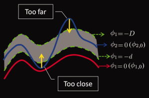
The proposed distance constraint term. The preferred range is indicated by the grey zone. [Color figure can be viewed in the online issue, which is available at wileyonlinelibrary.com.]

Since, for normal growth, major anatomical structures are preserved throughout the early brain developmental stages, we constrain the distance between the zero‐level sets of ϕ₁ (or ϕ₂) and ϕ${}_{\text{1}}^{\text{L}}$ (or ϕ${}_{\text{2}}^{\text{L}}$) to fall within a predefined range, based on the same idea of incorporating the distance constraint in Eqs. (3) and (4). We first consider ϕ₁, and let the allowed range be [d ₁ D ₁] with d ₁ < 0 and D ₁ > 0. Therefore, ϕ_1,0 should fall between the zero level sets of ϕ${}_{\text{1}}^{\text{L}}$ − d ₁ and ϕ${}_{\text{2}}^{\text{L}}$ − D ₁. We define the longitudinal constraint term as

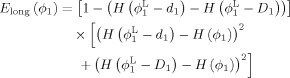(5)

 Similarly, for ϕ₂, let the allowed range be [d ₂ D ₂] with d ₂ < 0 and D ₂ > 0, and the respective longitudinal constraint term is

(6)

 The final energy function for the longitudinally guided level‐sets, combining the atlas prior, cortical thickness constraint, and longitudinal constraint is as follows:

(7)

where α and β are the blending parameters. It is worth noting that prior_i in E _{L_prior} is not a population atlas as in Eq. (2), but a subject‐specific atlas [Shi et al., 2010] which can be constructed from the warped brain tissue distributions of two‐year‐old (Year2). To effectively minimize this energy with respect to ϕ₁ and ϕ₂, we decompose equation (7) into the following

(8)

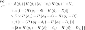
 By calculus of variations, the minimization of the energy functions with respect to ϕ₁, ϕ₂ and ϕ₃ are achieved by solving the gradient descent flow equations as follows

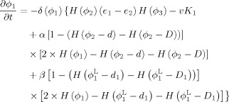(9)

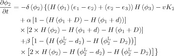(10)

(11)

where

(12)

and

(13)

Implementation

In practice, the Heaviside function H is approximated using a smooth function H _ε [Chan and Vese, 2001]

with derivative

 All the spatial partial derivatives , , and are approximated by the central difference. The energy term e _i (x) can be easily calculated by a convolution operation. The implementation of our method is straightforward. The whole process is summarized below:

Let

Step 1. Initial segmentation of Year2 and Year0 by using AFCM [Pham and Prince, 1999] and coupled level sets [Wang et al., 2011], respectively. Let the reconstructed zero‐level surfaces, representing the WM/GM and GM/CSF boundaries of Year2, as and , and Year0 as ϕ₁ and ϕ₂;

Step 2. On the basis of the segmentation results of Year2 and Year0, use HAMMER [Shen and Davatzikos, 2002] to warp and into Year0 space, resulting in ϕ${}_{\text{1}}^{\text{L}}$ and ϕ${}_{\text{2}}^{\text{L}}$;

Step 3. Longitudinally guided segmentation for Year0 to update ϕ₁,ϕ₂ and ϕ₃ according to Eqs. (9), (10), and (11):

Step 4. Return to Step 2 until the solution become stable, i.e., the tissue label difference between the newly updated segmentation in Step 3 and the previous segmentation is smaller than a certain threshold (such as 10 used for all experiments in this article).

EXPERIMENTAL RESULTS

Data were acquired using a 3T Siemens scanner. For the two‐year‐olds, T1 images with 160 axial slices were obtained with imaging parameters: TR = 1,900 ms, TE = 4.38 ms, Flip Angle = 7, acquisition matrix = 256 × 192, and resolution = 1 × 1 × 1 mm³. For the neonates, T2 images of 70 axial slices were obtained with imaging parameters: TR = 7,380 ms, TE = 119 ms, Flip Angle = 150, acquisition matrix = 256 × 128, and resolution = 1.25 × 1.25 × 1.95 mm³. All T2 images were resampled to 1 ×1 × 1 mm³. Before further processing, we employed the Brain Surface Extractor (BSE) [Shattuck and Leahy 2001) and the Brain Extraction Tool (BET) [Smith, 2002] to remove nonbrain tissues such as the skull and extracranial tissues. The results were then reviewed by a trained rater to manually edit, by using ITK‐SNAP3, the brain mask for removing extra non‐brain tissue and recovering over‐removed brain tissue.

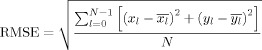
In our experiments, we set the allowable range cortical thickness of the neonatal brains to [1, 6.5] mm, the allowable range for the longitudinal constraint on cortical thickness to [−1.5, 1.5] mm, ε = 1.0, ν = 0.5, α = 0.25, and β = 0.5. The level‐sets functions are reinitialized as the signed distance functions at every iteration, by using a fast marching method [Sethian 1999). To measure the overlap rate between segmentations A and B, we employ Dice ratio, defined as DR (A,B) = 2|A ∩ B |/(|A| + |B|). DR ranges from 0 to 1, corresponding to the worst to best agreement between the labels. Besides the DR measure, we also use another commonly‐used measure such as surface distance for gauging segmentation error, which is defined as:

where surf (A) is the set of surface points of A, n _A is the total number of surface points in surf (A), and dist (a, A) is the Euclidean distance between a surface point a and the nearest surface point of A.

Effectiveness of the longitudinal constraint term

In this section, we will demonstrate the effectiveness of the longitudinal constraint term for neonatal segmentation. For simplicity, we use as example the GM/WM surface ϕ₂, by considering the energy function,

Fig. 5(a) is a synthetic image with constant cortical thickness, where the red curve indicates the ground truth for ϕ_2,0. Fig. 5(b) is a simulated neonatal (Year0) image obtained by blurring the first image with a Gaussian kernel (size = 3 × 3, standard deviation = 1) and adding Gaussian noise (standard deviation = 3). Fig. 5(c) is a synthetic two‐year‐old (Year2) image after being warped to the neonatal (Year0) space. Note that for this image, we deliberately made the cortex thicker and thinner at two different locations to simulate variation in cortical thickness due to cortical development or registration error. The second row, from left to right, shows the curve evolution for the case of β = 0 (see eq. (7)), i.e., without the longitudinal constraint term. It can be clearly seen that the final result is confounded at a local minima and is thus far from accurate. The third row shows the curve evolution for the case of β = 0.5 and d ₂ = D ₂ = 0, which implies that the longitudinal constraint is always applied. The blue curve denotes ϕ${}_{\text{L}}^{\text{2,0}}$, i.e., the longitudinal constraint from two‐year‐old (Year2). In this case, both information from the image and the longitudinal constraint are used to guide curve evolution. By setting d ₂ = D ₂ = 0, no distance tolerance is allowed for ϕ_2,0 with respect to the constraint curve, causing the evolved curve to be trapped between the ground‐truth and the constraint curves. In the last row, by setting d ₂ = −4, D ₂ = 4, the distance tolerance from the constraint curve is indicated by the two green dashed curves. The evolving curve is therefore given a greater flexibility to locate the ground‐truth curve, guided by the information given by the neonate image. For better comparison, we employ the root mean squared error (RMSE) to measure the distance between the evolved curves and the ground truth curve. Let the coordinates of the points on the evolved contour be (x ₀, y ₀), …, (x _{N − 1}, y _{N − 1}). For each (x _l, y _l), (l = 0, …, N − 1), we find its corresponding point (x_l, y_l), (l = 0, …, N − 1) on the ground‐truth curve with the closest distance to (x _l, y _l). The RMSE is then computed as follows:

The plot of RMSE values for the three different cases is shown in the same figure. This result indicates that the longitudinal constraint term plays an important role in locating the correct cortical boundaries.

Figure 5.

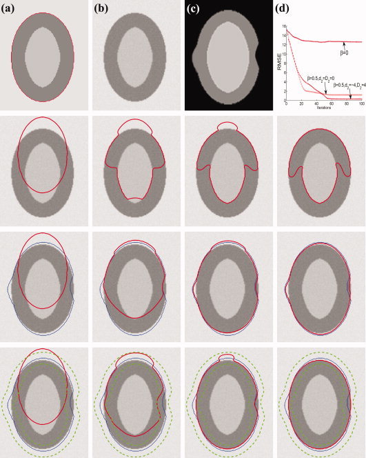
The effect of the longitudinal constraint term. The first row, from left to right, shows the ground truth (a), the synthetic neonatal image (b), the warped synthetic two‐year‐old image (c) and the RMSE plot. The second row shows the curve evolution without longitudinal constraint (β = 0). The third row shows the curve evolution with longitudinal constraint, but without zero distance tolerance (β = 0.5,d₂ = D₂ = 0). The last row shows the curve evolution with longitudinal constraint allowing distance tolerance, as marked by the two dashed green curves (β = 0.5, d₂ = −4 and D₂ = 4). [Color figure can be viewed in the online issue, which is available at wileyonlinelibrary.com.]

Simulated neonatal images

To demonstrate the advantage of the proposed method, we apply our method to a number of simulated neonatal images. The simulated image is generated by utilizing segmentation information from the Year2 image and intensity information from the Year0 image of a randomly selected subject. Details are given in the following. We denote the Year0 and Year2 intensity images of a selected subject as I ₀ and I ₂, and their respective segmented images as S ₀ and S ₂. Based on the segmented images S ₀ and S ₂, I ₀ is transformed, with the help of HAMMER [Shen and Davatzikos 2002), to the image space of I ₂, resulting in a warped image Ĩ ₀ (see Fig. 6). Since more reliable segmentation information can be obtained from S ₂ compared with S ₀, S ₂ is used to help generate the simulated image in our experiment. To generate a reasonable neonatal image with realistic tissue contrast, we borrow the intensity information from I ₀. To do this, for every voxel location P _i in the S ₂ space, we model the intensity distribution of its neighboring voxels in Ĩ ₀ using a simple Gaussian distribution. This is illustrated in the dashed box in Fig. 6, where the neighborhoods of voxel locations P ₁ and P ₂ are marked by the blue and red circles, respectively. We consider, for each voxel location P _i, only the neighboring voxels that are of the same tissue type (GM or WM) as that of voxel P _i, based on the segmentation information given by S ₂. A random value is then sampled at each point P _i from the estimated distribution to form the simulated image Ĩ ₂. To further ensure that the generated images are realistic, Ĩ ₂ and S ₂ are warped back to the Year0 image space, leading to much smaller size of brain than that in the Year2 space. This warping is achieved by a realistic simulated deformation field, which is constructed by using the method proposed by [Xue et al., 2006) after affine registering the Year2 intensity image Ĩ ₂ to any neonatal image. The warped Ĩ ₂ and S ₂ images are regarded as the simulated neonatal intensity image and the corresponding ground‐truth segmentation image.

Figure 6.

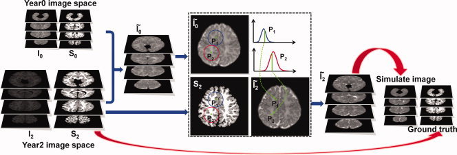
Simulating a set of neonatal images with ground‐truth segmentation images. [Color figure can be viewed in the online issue, which is available at wileyonlinelibrary.com.]

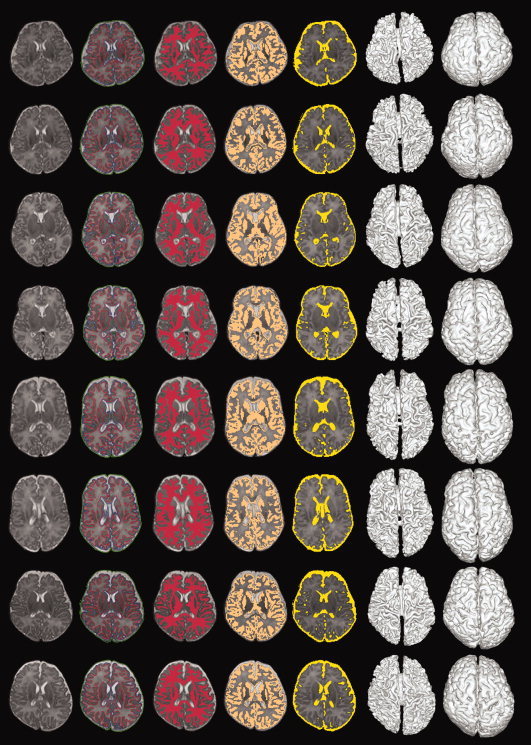
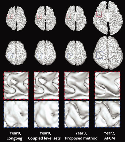
Using the method described above, 10 sets of longitudinal data are generated to evaluate the proposed method. Four representative slices from a simulated image and the corresponding ground‐truth segmentations are shown in the first and last columns of Fig. 7. The segmentation results of LongSeg [Shi et al., 2010) (a voxel‐based longitudinal segmentation method), coupled level sets [Wang et al., 2011) (a surface based segmentation method on a single‐time‐point image), and the proposed method (a surface based longitudinal segmentation method) are shown in columns 2, 3, and 4 of the figure, respectively. By visual inspection alone, it can be observed that the proposed method achieves more accurate results than the other two methods. Fig. 8 provides the corresponding 3D surfaces reconstructed from the segmentation images. The surfaces for the three methods mentioned above are shown in the first three columns, along with the surfaces of the Year2 segmentation image in the last column. The results obtained by the proposed method are more consistent with that of the Year2 segmentation image. This is especially apparent by looking at the zoomed views in the two bottom rows. Quantitative comparison based on the segmentations of all 10 simulated subjects is performed using the Dice ratio. As shown in Table I, the proposed method achieves the highest accuracy on both WM and GM.

Figure 7.

Comparison of segmentation results based on the simulated data set. From left to right are the simulated images, results given by LongSeg, the coupled level sets, the proposed method, and the ground truth.

Figure 8.

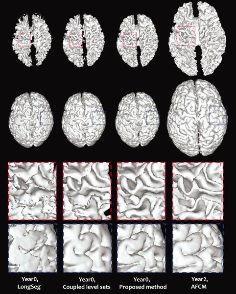
3D renderings of the WM/GM and GM/CSF surfaces based on the segmentation images. The last two rows show the zoomed views of regions marked by the rectangles. [Color figure can be viewed in the online issue, which is available at wileyonlinelibrary.com.]

Table I.

Comparison of the proposed method with the LongSeg and the coupled level sets on all 10 simulated subjects

		Methods
		LongSeg	Coupled level sets	Proposed method
Dice ratio	WM	0.844 ± 0.010	0.887 ± 0.006	0.945 ± 0.014
	GM	0.881 ± 0.006	0.901 ± 0.005	0.928 ± 0.007
Absolute surface Distance error (mm)	WM/GM	1.490 ± 0.149	0.919 ± 0.047	0.385 ± 0.091
	GM/CSF	0.789 ± 0.066	0.583 ± 0.034	0.414 ± 0.048

The first two rows of Fig. 9 show the distances from the surfaces obtained by the considered methods to the ground‐truth surfaces. Since the distance measure is not symmetrical, the distances from the ground‐truth surfaces to the obtained surfaces are also shown in the last two rows of the figure. It can be clearly seen that the proposed method agrees most with the ground truth. The histograms of the surface distance errors of WM/GM and GM/CSF surfaces are shown in Fig. 10, with the 95‐th percentile indicated by the bars at the top. Closer views of the plots are shown in the bottom row of the figure. As shown in Table I, the average absolute surface‐distance errors for WM/GM and GM/CSF surfaces obtained by the proposed method on all 10 simulated subjects are (0.39 ± 0.09, 0.41 ± 0.05) mm, along with (0.92 ± 0.05, 0.58 ± 0.30) mm by the coupled level sets and (1.49 ± 0.1, 0.79 ± 0.07) mm by LongSeg. Additionally, the Hausdorff distance, defined as

was also used to measure the maximal surface‐distance errors of each of 10 subjects. The average Hausdorff distance for WM/GM and GM/CSF on all 10 subjects obtained by the proposed method are (2.72 ± 0.51, 2.42 ± 0.34) mm, along with (5.89 ± 0.45, 4.36 ± 0.39) mm by the coupled level sets and (6.92 ± 0.65, 5.93 ± 0.56) mm by LongSeg, which again demonstrate the advantage of the proposed method.

Figure 9.

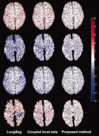
The first two rows show the surface distances from the surfaces obtained by the different methods to the ground‐truth surfaces; the last two rows show the distances from the ground‐truth surfaces to the estimated surfaces. [Color figure can be viewed in the online issue, which is available at wileyonlinelibrary.com.]

Figure 10.

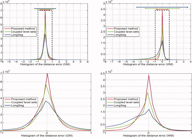
Histograms of the surface‐distance errors shown in Fig. 9. Top‐left: errors on GM/CSF surfaces; Top‐right: errors on WM/GM surfaces. Here, the errors from the ground‐truth surface to the obtained surface and the obtained surface to the ground‐truth surface are combined when calculating the histogram for the same GM/CSF surface (or WM/GM surface) by each segmentation method. The close‐up views are also shown in the bottom row. [Color figure can be viewed in the online issue, which is available at wileyonlinelibrary.com.]

In vivo neonatal subjects

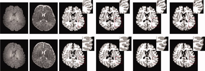
For validation of our method, images from 8 neonates, which are manually segmented, are used. The segmentation results yielded by our method are provided in Fig. 11 for visual inspection. The first column show the some exemplar slices of the original T2‐weighted images. The second column shows the segmentation results yielded by the proposed method. To better visualization, the hard segmentation results for WM, GM and CSF are also shown in columns 3, 4, and 5, respectively. These results indicate that the WM, GM and CSF are reasonably segmented. The last two columns show the 3D renderings of the WM/GM and GM/CSF surfaces.

Figure 11.

Segmentation results by the proposed method. From left to right: different slices of the original MR T2‐weighted image, results given by the proposed method, WM, GM, CSF segmentations, and 3D rendering of WM/GM and GM/CSF surfaces. [Color figure can be viewed in the online issue, which is available at wileyonlinelibrary.com.]

Validation of the automatic segmentation algorithms is often difficult due to the unavailability of the ground truth. To overcome this problem, we use a set of manual segmentations as the golden standard. The boundaries of neonatal images may be quite fuzzy at some locations. For these fuzzy locations, especially the central subconrtical regions, which usually have a low contrast, the neuroanatomist will use the aligned Year2 image as a reference to delineate the boundaries. The MR T1‐ and T2‐weighted images of two representative subjects are shown in the first two columns of Fig. 12, with their respective manual segmentations shown in the last column. The segmentation results obtained by the LongSeg, the coupled level sets, and the proposed method are shown in the columns 3, 4, and 5, respectively. It can be observed that our results are comparable with those produced by expert. Fig. 13 shows the 3D renderings of the WM/GM surfaces and GM/CSF surfaces for the second subject, together with the Year2 surfaces shown in the last column. From the zoomed views in the two bottom rows, it can be seen that holes and handles can be found in the surfaces generated with LongSeg and the coupled level sets, while the results of the proposed method are more reasonable and consistent with the Year2 results. Taking the manual segmentation as ground truth, we conduct a quantitative comparison. The mean and standard deviation of Dice ratio values of the WM and GM segmentations of all 8 subjects are reported in Table II. The proposed method achieves the highest Dice ratio values for both WM and GM. The cortical surface distance errors, which are also included in the same table, are also favorable to the proposed method.

Figure 12.

2D slices comparison on real subjects. From left to right: The original T1‐ and T2‐weighted images, results of LongSeg, coupled level sets, the proposed method, and the ground truth. [Color figure can be viewed in the online issue, which is available at wileyonlinelibrary.com.]

Figure 13.

3D renderings of the WM/GM surfaces. The last two rows show the zoomed views of the first two rows. [Color figure can be viewed in the online issue, which is available at wileyonlinelibrary.com.]

Table II.

Comparisons of the proposed method with the LongSeg and the coupled level sets on eight real neonatal images

		Methods
		LongSeg	Coupled level sets	Proposed method
Dice ratio	WM	0.871 ± 0.019	0.911 ± 0.024	0.949 ± 0.009
	GM	0.864 ± 0.019	0.898 ± 0.020	0.919 ± 0.014
Absolute surface distance error (mm)	WM/GM	1.269 ± 0.123	0.680 ± 0.129	0.464 ± 0.086
	GM/CSF	0.890 ± 0.077	0.678 ± 0.085	0.554 ± 0.066

The effect of different initialization schemes

In this section, instead of using the coupled level sets, we employ LongSeg to generate an initial segmentation of the neonatal brain images for investigating how the initialization will influence the final segmentation results. Tissue overlap comparison on 10 simulated subjects and 8 real subjects are shown in Fig. 14(a) and Fig. 14(b), respectively. Here, “Proposed A” and “Proposed B” denote segmentation using the longitudinally guided level‐sets based method with initialization provided by LongSeg and the coupled level sets, respectively. As shown in Fig. 14(a), the “Proposed B” achieves a slightly higher accuracy than “Proposed A” for the simulated data. The main reason for this improvement is due to the fact that better initial segmentation is conducive to more accurate alignment using HAMMER between the neonatal image and the longitudinal scan, and thus allows more accurate guidance for segmentation. The same conclusion can be made using the real data, as can be observed from Fig. 14(b).

Figure 14.

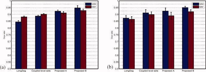
The effect of different initialization schemes on the final segmentation accuracy. “Proposed A” and “Proposed B” denote segmentation using the longitudinally guided level‐sets based method with initialization provided by LongSeg and the coupled level sets, respectively. Left: results on simulated data; Right: results on real data. [Color figure can be viewed in the online issue, which is available at wileyonlinelibrary.com.]

Comparison between segmentation propagation and the proposed method

Simple segmentation propagation from Year2 to Year0 is incapable of producing accurate results. The proposed method employs the propagated segmentation as a subject‐specific prior for further improving segmentation accuracy. Representative results are shown in Fig. 15, where from left to right are the segmentation propagated from Year2, the segmentation given by the proposed method, and ground truth, respectively. It can be observed that the proposed method produces more accurate results than the simple segmentation propagation approach, especially at locations indicated by the yellow arrows. The average Dice ratios for WM and GM of the simple segmentation propagation approach, computed based on all 10 simulated subjects, are 0.85 ± 0.01 and 0.86 ± 0.01. Recall that the average Dice ratios for WM and GM of the proposed method are 0.94 ± 0.01 and 0.92 ± 0.01, respectively, which quantitatively show the better performance of the proposed method.

Figure 15.

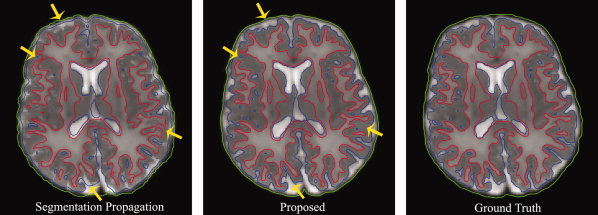
Comparison between the simple segmentation propagation approach (left) and the proposed method (middle). Ground‐truth segmentation for the simulated data is shown in the right. [Color figure can be viewed in the online issue, which is available at wileyonlinelibrary.com.]

DISCUSSION AND CONCLUSION

In conclusion, we have proposed a novel longitudinally guided level‐sets based method for consistent neonatal image segmentation. The longitudinal information is incorporated in the segmentation framework via a new distance constraint term. The proposed method, validated on both simulated and in vivo neonatal brain images, shows very promising results compared with existing state‐of‐the‐art methods.

Although there exist many linear (FLIRT4) and nonlinear (ANTS [Avants et al., 2008], ARTS5, DEMONS [Beg et al., 2005]) registration methods, we adopt in this paper the HAMMER registration method [Shen and Davatzikos, 2002] to warp the segmentation image of the Year2 to the respective neonatal image due to the following reasons. First, the brain development is not linear. For example, as reported, the sensorimotor cortex matures earliest, with parietal and temporal association cortex maturing next and the prefrontal cortex maturing last [Casey et al., 2005). Therefore, linear methods such as FLIRT method cannot adequately capture the deformation. Second, image contrast changes dramatically in the early brain development and thus methods that are based directly on image intensity, such as sum of squared intensity differences (SSD), are prone to fail. Third, the HAMMER [Shen and Davatzikos 2002), which is an elastic registration method, is specifically proposed for registration of the segmented images, and hence does not depend directly on the intensity images that can be very different for the neonatal and one‐year‐old or two‐year‐old images. To support our argument and also for fair comparison with other registration methods, in our experiments we also tested DEMONS on both segmented images (DEMONS1) and original intensity images (DEMONS2). Similarly, we applied ARTS on both segmented images (ARTS1) and original intensity images (ARTS2). For ANTS, we tested it on the segmented images using the mean square difference (ANTS1) and also on the original intensity images using mutual information (ANTS2). We found that HAMMER allows to achieve more accurate results than any other method in neonatal segmentation as confirmed by both visual inspection and quantitative evaluation. For quantitative evaluation, we compared the automated segmentation with manual segmentation using the Dice ratio. In particular, the Dice ratios for WM and GM on eight infant subjects are 0.80 ± 0.01 and 0.80 ± 0.01 by DEMONS1, 0.55 ± 0.05 and 0.62 ± 0.03 by DEMONS2; 0.83 ± 0.01 and 0.82 ± 0.01 by ANTS1, 0.63 ± 0.04 and 0.64 ± 0.03 by ANTS2; 0.81 ± 0.01 and 0.82 ± 0.01 by ARTS1, 0.52 ± 0.05 and 0.57 ± 0.04 by ARTS2; 0.85 ± 0.01 and 0.86 ± 0.01 by HAMMER. It can be seen that HAMMER achieves the best results, and also for each other method the results on using segmented images for guiding registration are much better than those using the original intensity images, since the registration on the original intensity images are often more difficult due to dynamic intensity changes in early brain development.

In this article, the Year0 segmentation is guided by the Year2 segmentation, and thus could be potentially biased by the Year2 segmentation if the major structures in Year0 are very different from those in Year2. Fortunately, for the full‐term infants, the patterns of major sulci and gyri are already present from birth and do not change dramatically during the early brain development, thus this potential bias on Year0 segmentation can be minimized.

Future work entails evaluating the proposed method based on the increasing amount of data sets actively acquired at our institute. We note that although the results are promising, the current implementation does not guarantee that the estimated cortical surface is topologically equivalent to a sphere. To remedy this, the existing topology correction methods [Han et al., 2004) can be incorporated in our current method. Future work will be directed to resolve this limitation.

REFERENCES

- Abe S, Takagi K, Yamamoto T, Okuhata Y, Kato T ( 2003): Assessment of cortical gyrus and sulcus formation using MR images in normal fetuses. Prenat Diagn 23: 225–231. [DOI] [PubMed] [Google Scholar]
- Aljabar P, Heckemann RA, Hammers A, Hajnal JV, Rueckert D ( 2009): Multi‐atlas based segmentation of brain images: Atlas selection and its effect on accuracy. NeuroImage 46: 726–738. [DOI] [PubMed] [Google Scholar]
- Almlia CR, Rivkinb MJ, McKinstryc RC; Brain Development Cooperative Group ( 2007): The NIH MRI study of normal brain development (Objective‐2): Newborns, infants, toddlers, and preschoolers. NeuroImage 35: 308–325. [DOI] [PubMed] [Google Scholar]
- Armstrong E, Schleicher A, Omran H, Curtis M, Zilles K ( 1995): The ontogeny of human gyrification. Cerebral Cortex 5: 56–63. [DOI] [PubMed] [Google Scholar]
- Avants BB, Epstein CL, Grossman M, Gee JC ( 2008): Symmetric diffeomorphic image registration with cross‐correlation: Evaluating automated labeling of elderly and neurodegenerative brain. Med Image Anal 12: 26–41. [DOI] [PMC free article] [PubMed] [Google Scholar]
- Awate S, Tasdizen T, Foster N, Whitaker R ( 2006): Adaptive Markov modeling for mutual‐information‐based, unsupervised MRI brain‐tissue classification. Med Image Anal 10: 726–739. [DOI] [PubMed] [Google Scholar]
- Beg MF, Miller MI, Trouvé A, Younes L ( 2005): Computing large deformation metric mappings via geodesic flows of diffeomorphisms. Int J Comput Vis 61: 139–157. [Google Scholar]
- Bhatia KK, Hajnal JV, Puri BK, Edwards AD, Rueckert D ( 2004): Consistent groupwise non‐rigid registration for atlas construction. Proc IEEE Symp Biomed Imaging, ISBI. pp 908–911. [Google Scholar]
- Casey B, Tottenham N, Liston C, Durston S ( 2005): Imaging the developing brain: What have we learned about cognitive development? Trends Cogn Sci 9: 104–110. [DOI] [PubMed] [Google Scholar]
- Chan T, Vese L ( 2001): Active contours without edges. IEEE Trans Imag Proc 10: 266–277. [DOI] [PubMed] [Google Scholar]
- Chi J, Dooling E, Gilles F ( 1977): Gyral development of the human brain. Ann Neurol 1: 86–93. [DOI] [PubMed] [Google Scholar]
- Cocosco CA, Zijdenbos AP, Evans AC ( 2003): A fully automatic and robust brain MRI tissue classification method. Med Image Anal 7: 513–527. [DOI] [PubMed] [Google Scholar]
- Cremers D, Rousson M, Deriche R ( 2007): A review of statistical approaches to level set segmentation: integrating color, texture, motion and shape. Int J Comp Vis 72: 195–215. [Google Scholar]
- Dubois J, Benders M, Cachia A, Lazeyras F, Ha‐vinh R, Sizonenko SV, Borradori‐tolsa C, Mangin JF ( 2008): Mapping the early cortical folding process in the preterm newborn brain. Cerebral Cortex 18: 1444–1454. [DOI] [PubMed] [Google Scholar]
- Gerig G, Davis B, Lorenzen P, Xu S, Jomier M, Piven J, Joshi S ( 2006): Computational Anatomy to Assess Longitudinal Trajectory of Brain Growth. 3DPVT ′06: Proceedings of the Third International Symposium on 3D Data Processing, Visualization, and Transmission (3DPVT′06). Washington, DC, USA: IEEE Computer Society; pp 1041–1047. [Google Scholar]
- Goldenberg R, Kimmel R, Rivlin E, Rudzsky M ( 2002): Cortex segmentation: A fast variational geometric approach. IEEE Trans Med Imag 21: 1544–1551. [DOI] [PubMed] [Google Scholar]
- Gooya A, Liao H, Matsumiya K, Masamune K, Masutani Y, Dohi T ( 2008): A variational method for geometric regularization of vascular segmentation in medical images. IEEE Trans Image Proc 17: 1295–1312. [DOI] [PubMed] [Google Scholar]
- Guillemaud R, Brady J ( 1997): Estimating the bias field of MR images. IEEE Trans Med Imag 16: 238–251. [DOI] [PubMed] [Google Scholar]
- Han X, Pham DL, Tosun D, Rettmann ME, Xu C, Prince JL ( 2004): CRUISE: Cortical reconstruction using implicit surface evolution. NeuroImage 23: 997–1012. [DOI] [PubMed] [Google Scholar]
- Hill J, Dierker D, Neil J, Inder T, Knutsen A, Harwell J, Coalson T, Van Essen D ( 2010): A surface‐based analysis of hemispheric asymmetries and folding of cerebral cortex in term‐born human infants. J Neurosci 10: 2268–2276. [DOI] [PMC free article] [PubMed] [Google Scholar]
- Knickmeyer RC, Gouttard S, Kang C, Evans D, Wilber K, Smith JK, Hamer RM, Lin W, Gerig G, Gilmore JH ( 2008): A structural MRI study of human brain development from birth to 2 years. J Neurosci 28: 12176–12182. [DOI] [PMC free article] [PubMed] [Google Scholar]
- Kuklisova‐Murgasova M, Aljabar P, Srinivasan L, Counsell SJ, Doria V, Serag A, Gousias IS, Boardman JP, Rutherford MA, Edwards AD, et al. ( 2010): A dynamic 4D probabilistic atlas of the developing brain. NeuroImage 54: 2750–2763. [DOI] [PubMed] [Google Scholar]
- Lebel C, Walker L, Leemans A, Phillips L, Beaulieu C ( 2008): Microstructural maturation of the human brain from childhood to adulthood. Neuroimage 40: 1044–1055. [DOI] [PubMed] [Google Scholar]
- Leemput V, Maes K, Vandermeulen D, Suetens P ( 1999): Automated model‐based bias field correction of MR images of the brain. IEEE Trans Med Imag 18: 885–896. [DOI] [PubMed] [Google Scholar]
- Li C ( 2006): Active contours with local binary fitting energy. IMA Workshop on New Mathematics and Algorithms for 3‐D Image Analysis.
- Li C, Huang R, Ding Z, Gatenby C, Metaxas D, Gore J ( 2008a): A Variational Level Set Approach to Segmentation and Bias Correction of Medical Images with Intensity Inhomogeneity. MICCAI. pp 1083–1091. [DOI] [PMC free article] [PubMed]
- Li C, Kao C, Gore J, Ding Z ( 2007): Implicit active contours driven by local binary fitting energy. CVPR. pp 1–7. [Google Scholar]
- Li C, Kao C, Gore JC, Ding Z ( 2008b): Minimization of region‐scalable fitting energy for image segmentation. IEEE Trans Image Process 17: 1940–1949. [DOI] [PMC free article] [PubMed] [Google Scholar]
- Li C, Li F, Kao C‐Y, Xu C ( 2009): Image segmentation with simultaneous illumination and reflectance estimation: An energy minimization approach. ICCV. pp 702–708 [Google Scholar]
- MacDonald D, Kabani N, Avis D, Evans AC ( 2000): Automated 3‐D extraction of inner and outer surfaces of cerebral cortex from MRI. NeuroImage 12: 340–356. [DOI] [PubMed] [Google Scholar]
- Osher S, Sethian J ( 1988): Fronts propagating with curvature‐dependent speed: Algorithms based on Hamilton‐Jacobi formulations. J Comp Phys 79: 12–49. [Google Scholar]
- Pham DL, Prince JL ( 1999): Adaptive fuzzy segmentation of magnetic resonance images. IEEE Trans Med Imaging 18: 737–752. [DOI] [PubMed] [Google Scholar]
- Prastawa M, Gilmore JH, Lin W, Gerig G ( 2005): Automatic segmentation of MR images of the developing newborn brain. Medical Image Anal 9: 457–466. [DOI] [PubMed] [Google Scholar]
- Rousson M, Cremers D ( 2005): Efficient kernel density estimation of shape and intensity priors for level set segmentation. MICCAI. pp 757–764. [DOI] [PubMed] [Google Scholar]
- Sethian J ( 1999): Level Set Methods and Fast Marching Methods. Cambridge: Cambridge University Press. [Google Scholar]
- Shattuck DW, Leahy RM ( 2001): Automated graph‐based analysis and correction of cortical volume topology. Med Imaging IEEE Trans 20: 1167–1177. [DOI] [PubMed] [Google Scholar]
- Shen D, Davatzikos C ( 2002): HAMMER: Hierarchical attribute matching mechanism for elastic registration. IEEE Trans Med Imaging 21: 1421–1439. [DOI] [PubMed] [Google Scholar]
- Shi F, Fan Y, Tang S, Gilmore JH, Lin W, Shen D ( 2010): Neonatal brain image segmentation in longitudinal MRI studies. NeuroImage 49: 391–400. [DOI] [PMC free article] [PubMed] [Google Scholar]
- Shi F, Yap P‐T, Wu G, Jia H, Gilmore JH, Lin W, Shen D ( 2011): Infant brain atlases from neonates to 1‐ and 2‐year‐olds. PLoS One 6: e18746. [DOI] [PMC free article] [PubMed] [Google Scholar]
- Smith SM ( 2002): Fast robust automated brain extraction. Hum Brain Mapp 17: 143–155. [DOI] [PMC free article] [PubMed] [Google Scholar]
- Song Z, Awate SP, Licht DJ, Gee JC ( 2007): Clinical neonatal brain mri segmentation using adaptive nonparametric data models and intensity‐based markov priors. MICCAI. pp 883–890. [DOI] [PubMed] [Google Scholar]
- Thompson D, Warfield S, Carlin J, Pavlovic M, Wang H, Bear M, Kean M, Doyle L, Egan G, Inder T ( 2007): Perinatal risk factors altering regional brain structure in the preterm infant. Brain 130: 667–677. [DOI] [PubMed] [Google Scholar]
- Wang L, He L, Mishra A, Li C ( 2009): Active contours driven by local gaussian distribution fitting energy. Signal Proc 89: 2435–2447. [Google Scholar]
- Wang L, Shi F, Lin W, Gilmore JH, Shen D ( 2011): Automatic segmentation of neonatal images using convex optimization and coupled level sets. NeuroImage 58: 805–817. [DOI] [PMC free article] [PubMed] [Google Scholar]
- Warfield SK, Kaus M, Jolesz FA, Kikinis R ( 2000): Adaptive, template moderated, spatially varying statistical classification. Med Image Anal 4: 43–55. [DOI] [PubMed] [Google Scholar]
- Weisenfeld NI, Mewes AUJ, Warfield SK ( 2006): Segmentation of newborn brain MRI. Biomedical Imaging: Nano to Macro, 2006. 3rd IEEE International Symposium on. p 766–769.
- Weisenfeld NI, Warfield SK ( 2009): Automatic segmentation of newborn brain MRI. NeuroImage 47: 564–572. [DOI] [PMC free article] [PubMed] [Google Scholar]
- Wells W, Grimson E, Kikinis R, Jolesz F ( 1996): Adaptive segmentation of MRI data. IEEE Trans Med Imag 15: 429–442. [DOI] [PubMed] [Google Scholar]
- Xu C, Pham DL, Rettmann ME, Yu DN, Prince JL ( 1999): Reconstruction of the human cerebral cortex from magnetic resonance images. IEEE Trans Med Imag 18: 467–480. [DOI] [PubMed] [Google Scholar]
- Xue H, Srinivasan L, Jiang S, Rutherford M, Edwards AD, Rueckert D, Hajnal JV ( 2007): Automatic segmentation and reconstruction of the cortex from neonatal MRI. NeuroImage 38: 461–477. [DOI] [PubMed] [Google Scholar]
- Xue Z, Shen D, Karacali B, Stern J, Rottenberg D, Davatzikos C ( 2006): Simulating deformations of MR brain images for validation of atlas‐based segmentation and registration algorithms. NeuroImage 33: 855–866. [DOI] [PMC free article] [PubMed] [Google Scholar]
- Yezzi A, Paragios N, Deriche R ( 2000): Geodesic active contours and level sets for detection and tracking of moving objects. IEEE Trans Patt Anal Mach Intell 22: 266–280. [Google Scholar]
- Zeng X, Staib L, Schultz R, Duncan J ( 1999): Segmentation and measurement of the cortex from 3D MR images using coupled surfaces propagation. IEEE Trans Med Imag 18: 100–111. [DOI] [PubMed] [Google Scholar]