Evaluation of models of spectral distortions in photon-counting detectors for computed tomography

Abstract.

A semi-analytical model describing spectral distortions in photon-counting detectors (PCDs) for clinical computed tomography was evaluated using simulated data. The distortions were due to count rate-independent spectral response effects and count rate-dependent pulse-pileup effects and the model predicted both the mean count rates and the spectral shape. The model parameters were calculated using calibration data. The model was evaluated by comparing the predicted x-ray spectra to Monte Carlo simulations of a PCD at various count rates. The data-model agreement expressed as weighted coefficient of variation $({\mathrm{COV}}_{\mathrm{W}})$ was better than ${\mathrm{COV}}_{\mathrm{W}}=2.0\%$ for dead time losses up to 28% and ${\mathrm{COV}}_{\mathrm{W}}=20\%$ or smaller for dead time losses up to 69%. The accuracy of the model was also tested for the purpose of material decomposition by estimating material thicknesses from simulated projection data. The estimated attenuator thicknesses generally agreed with the true values within one standard deviation of the statistical uncertainty obtained from multiple noise realizations.

1. Introduction

Photon-counting detectors (PCDs) are a promising technology for clinical computed tomography (CT) with the potential to reduce noise and dose, improve tissue identification, and enable functional CT imaging.^1–6 The many advantages are challenged by distortions that real PCDs introduce to the measurement of the photon energy spectrum transmitted through an object. These distortions can be divided into two main categories: (1) spectral distortions from the energy response of the detector, which are independent of the count rate and (2) spectral distortions due to the limited count rate capability of the detector, which are dependent on the photon fluence and are attributed to photon pulse pileup.^7–13 The successful application of PCDs for clinical CT requires a good understanding of the nature of the distortions and computationally inexpensive algorithms to correct or compensate for them before or during image reconstruction.¹

In a recent publication, a semi-analytical, cascaded model of spectral distortions was proposed.⁸ This model is capable of modeling the measured photon spectra of a particular paralyzable PCD with high accuracy over a large range of count rates. Many other designs of PCDs for clinical x-ray imaging have been explored in the literature (for an overview see Table 1 in Ref. 1). The amount of spectral distortions is critically determined by the choice of sensor material, pixel size and thickness, and the design of the readout electronics, which influences the detector dead time and the extent of spectral distortions due to photon pileup. The purpose of this paper was to demonstrate that the cascaded model is adaptable for detectors with different geometry (smaller pixel size), pulse shapes (unipolar), smaller dead times, and nonparalyzable detection mechanism. An improvement made to the pulse-pileup model now allows for energy-dependent dead times. We validated the model by comparing photon energy spectra from Monte Carlo (MC) simulations of different detector designs to the predictions from our model for various count rates. One of the major advantages of PCDs is the ability to identify multiple tissues from a single scan. Successful material decomposition in clinical conditions using model-based approaches, therefore, requires an accurate model of the PCD. In another aspect of this study, we tested the applicability of the model for material decomposition by assessing the accuracy of estimating the thicknesses of simulated attenuator materials and comparing the results to the true thickness values.

Table 1.

Attenuators used in the simulation.

Attenuators	Set A (mm)	Set B (mm)
Al	3.5	3.5
Ti	0.9	0.9
${\mathrm{H}}_2\mathrm{O}$	100.0	100.0
Gd	—	0.075

2. Cascaded Model of Spectral Distortions

The cascaded model is described in detail in Ref. 8, and only the main features and modifications are mentioned here. The model separates the complex phenomena of spectral distortions in PCDs into count rate-independent spectral response effects (SRE) and count rate-dependent pulse-pileup effects (PPE). SRE and PPE are modeled independently and the two models are cascaded to produce the final spectrum. Each of SRE and PPE describes a part of complex, integrated phenomena in a simplistic way. For example, as described in Ref. 1, SRE may produce two electron charges via K-escape x-rays from a photon, which could quasi-coincidentally be incident onto the same PCD pixel, producing an integrated pulse similar to PPE. Furthermore, the integrated pulse may overlap with a pulse from another photon (or photons) when the count rates are high. Nonetheless, the cascaded model appears to capture the major parts of the detection processes with sufficient accuracy.⁸

The SRE model requires as an input a finely binned, two-dimensional (2-D) matrix $A_{\mathrm{SRE}}$ of the detector’s measured photon energy spectrum at low count rates for monochromatic input energies over the applicable energy range. This matrix can be obtained, e.g., by recording the spectra of a small number of radioisotopes and interpolating the parameterization results in the required energy range, as was done in Ref. 8, or by accurate MC simulations of the detector. The SRE-distorted spectrum $S_{\mathrm{SRE}}(E)$ is calculated as

$$S_{\mathrm{SRE}}(E)={\mathrm{\Omega }}_{\mathrm{SRE}}[S_{\mathrm{t}}(E)]\text{or}{\overrightarrow{s}}_{\mathrm{SRE}}(E)=A_{\mathrm{SRE}}·{\overrightarrow{s}}_{\mathrm{t}}(E),$$ (1)

where on the left, $S_{\mathrm{t}}(E)$ is the spectrum transmitted through the attenuators (incident onto the detector) and ${\mathrm{\Omega }}_{\mathrm{SRE}}[S_{\mathrm{t}}(E)]$ is the operator that models the distortions due to SRE. On the right, the two spectra are described as vectors ${\overrightarrow{s}}_{\mathrm{SRE}}$ and ${\overrightarrow{s}}_{\mathrm{t}}$ and the SRE as a matrix $A_{\mathrm{SRE}}$. Given an incident photon count rate $a_{\mathrm{t}}$ (integrated over the whole photon energy range), the count rate as a function of energy measured by the detector, if PPE is negligible then

$$a_{\mathrm{SRE}}(E)=a_{\mathrm{t}}·S_{\mathrm{SRE}}(E).$$ (2)

The PPE model¹³ uses three conditional probabilities $f_{\mathrm{cnt}}$, $f_m$, and $f_E$ to calculate the spectral distortions due to pulse pileup that occurs at higher photon count rates. The recorded count rate is

$$a_{\mathrm{SRE}+\mathrm{PPE}}(E;a_{\mathrm{t}},{\tau }_0,a_{\mathrm{SRE}})=a_{\mathrm{t}}·f_{\mathrm{cnt}}(a_{\mathrm{t}},{\tau }_0)·\sum _m{f}_m(m;a_{\mathrm{t}},{\tau }_0)·f_E(E;m,a_{\mathrm{SRE}}),$$ (3)

where $f_{\mathrm{cnt}}$ is the probability for an event to be recorded (which is different for a paralyzable and nonparalyzable detector), $f_m$ is the probability that $m+1$ photons pile up and result in only one count, and $f_E$ is the probability that counts are recorded at energy $E$. The latter probability utilizes the pulse shape of the detector signal caused by a single photon, the probability distribution of time intervals between photons, and the probability density function of the spectrum $S_{\mathrm{SRE}}$.

In Eq. (3), the dead time ${\tau }_0$ is a fixed number, which was obtained from calibration measurements as described later. However, for an actual paralyzable detector, the detection mechanism is typically that of a pulse height analyzer (PHA), and the dead time depends on the threshold and the pulse height, hence, on the photon energy. The PHA becomes inactive if the pulse height rises above the energy threshold and remains inactive for as long the pulse height stays above the threshold. We modified the model to obtain a more accurate spectral shape by introducing an energy-dependent dead time $\tau (E)$ for the probabilities that describe the energy-dependent part of the PPE model. The expression in Eq. (3) was replaced as follows:

$$\begin{gathered} a_{\mathrm{SRE}+\mathrm{PPE}}[E;a_{\mathrm{t}},{\tau }_0,\tau (E),a_{\mathrm{SRE}}]=a_{\mathrm{t}}·f_{\mathrm{cnt}}(a_{\mathrm{t}},{\tau }_0)·\frac{f_{mE}(E)}{\int f_{mE}(E)\mathrm{d}E}, \\ \text{with}{f}_{mE}(E)=\sum _m{f}_m[m;a_{\mathrm{t}},\tau (E)]·f_E(E;m,a_{\mathrm{SRE}}). \end{gathered}$$ (4)

The choice of $\tau (E)$ depends on the specific detector model and is described in Secs. 3.1.4 and 4.1.2.

An additional model parameter is the scaling factor $k_0$ that relates the photon count rate per ${\mathrm{mm}}^2$, $a_0$, exiting the x-ray tube to the tube current $I$, $a_0=k_{0}I$. The original model was validated for a paralyzable detector with a bipolar pulse shape, where the negative pulse was shallow but long.^8,13 In this paper, we study a detector with unipolar pulse shape, smaller pixel size, and smaller dead time.

3. Methods

3.1. Model Evaluation

3.1.1. Simulation of photon-counting data

The model was compared to simulated data obtained from MC calculations. Using simulated data allow testing various detector configurations without having to design and build a corresponding physical detector. The agreement between the MC simulation and measured data from a prototype PCD has been investigated in Ref. 14. Details about the simulation package can also be found in Ref. 15. In short, the software simulates the photoelectric effect, Compton scatter, fluorescence, charge propagation due to the electric bias field, formation of the signal pulse, noise, charge sharing, and cross talk between pixels.

X-ray source spectrum

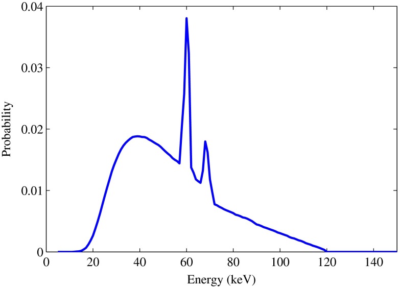
A 120-kVp source spectrum $S_0(E)$ was simulated for a tungsten anode and 2.0-mm aluminum filtration in the energy range between 5 and 150 keV in steps of 1 keV (Fig. 1).

Fig. 1.

The simulated 120-kVp input spectrum, including 2.0-mm Al filtration.

Attenuators

Data were simulated for two sets of attenuators as shown in Table 1. The sets A and B differ only by the additional attenuation by gadolinium in set B. The attenuators were homogeneous materials parallel to the surface of the curved detector. Scatter in the attenuators was not included in the simulation.

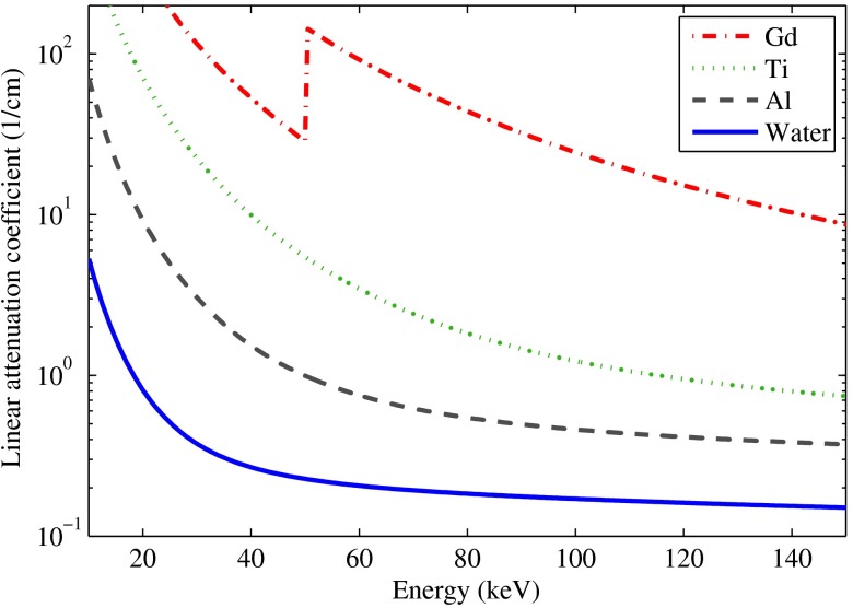
The linear attenuation coefficients for water, aluminum, titanium, and gadolinium were calculated using the EPDL library¹⁶ and are shown in Fig. 2 in the energy range between 10 and 150 keV. Aluminum was considered to be an intrinsic component of the x-ray tube (see also Sec. 3.1.4). The count rates for a 120-kVp x-ray spectrum were reduced by the attenuators (excluding aluminum) by a factor of 0.078 for set A and by a factor of 0.050 for set B.

Fig. 2.

Linear attenuation coefficients as a function of energy for the materials used in the simulation data sets.

Detector

A CdTe detector was simulated with $736\times 25$ macropixels in the column and row directions, respectively. Each macropixel consisted of $5\times 4$ micropixels, whose counts were added to provide the output of one macropixel. The fifth micropixel in the column direction did not output any counts and simulated the presence of antiscatter blades completely blocking the x-ray flux along every fifth column of the micropixels. Therefore, each macropixel consisted of $4\times 4$ active micropixels. Each micropixel had a dimension of $0.225\mathrm{mm}\times 0.225\mathrm{mm}\times 1.6\mathrm{mm}$, resulting in an active area of $0.81{\mathrm{mm}}^2$ for each macropixel. About ${10}^6$ photons were generated per micropixel before attenuation. The simulated frame time (also denoted as “reading”) was $868\mu \mathrm{s}$. The pulses in each micropixel were sampled by comparators connected to counters, and the comparator energy thresholds were changed from 5 to 240 keV in steps of 5 keV.

Pulse shape

A unipolar pulse shape was simulated using a truncated Gaussian pulse response function with full width at half maximum of 15 ns (this corresponds to a standard deviation of 6.4 ns). The pulse was clipped at $\pm 5$ standard deviations from the maximum for computational reasons.

Detector models

The counts in each counter were increased if the pulse height surpassed the comparator threshold on the rising part of the pulse. Counters became active again when the pulse height fell below their threshold.

The paralyzable detector was realized by leaving the counters in an inactive state as long as the pulse height was above the threshold. No additional photons were registered, while the detector was in this inactive state. The nonparalyzable detector was realized using a 25-MHz clock. The counter was repeatedly increased every 40 ns by one count as long as the pulse height was still above the threshold. In both detector models, the dead time, therefore, depended on the threshold level and pulse shape.

Simulated data sets

Data were simulated for the following configurations:

• a.attenuation with $3.5\mathrm{mm}\mathrm{Al}+0.9\mathrm{mm}\mathrm{Ti}+100.0\mathrm{mm}{\mathrm{H}}_2\mathrm{O}$ (set A),
• b.attenuation with $3.5\mathrm{mm}\mathrm{Al}+0.9\mathrm{mm}\mathrm{Ti}+100.0\mathrm{mm}{\mathrm{H}}_2\mathrm{O}+0.075\mathrm{mm}$ Gd (set B),
• c.detector: paralyzable and nonparalyzable,
• d.pulse shape: unipolar,
• e.tube currents: 25, 50, 100, 200, 400, 800, 1600, 3200, and 6400 mA at a tube voltage of 120 kV,
• f.photon energy thresholds: 5 to 240 keV in steps of 5 keV.

The total number of simulated data sets was 1728 (2 sets of attenuators, 2 detector schemes, 1 pulse shape, 9 tube currents, and 48 energy thresholds). For computational reasons, only one noise realization per data set was simulated. However, for the purpose of model evaluation, it is desirable to have multiple, uncorrelated noise realizations. Since, the detector consisted of $736\times 25=\mathrm{18,400}$ macropixels with identical simulation parameters, a subset of all available macropixels was chosen and treated as multiple noise realization of the same pixel. Care was taken when selecting an uncorrelated subset of pixels; charge sharing creates correlation between nearby pixels, and sufficient separation is required. Pixels near or on the edge of the detector may have a different energy response than the bulk of the pixels because of a reduced number of nearby pixels, which lowers the probability of cross talk from charge sharing. Therefore, only pixels were chosen that were separated by five macropixels from the next one and which were at least three pixels away from any edge.

Furthermore, two pixel subsets were selected: set $S_1$ to estimate the model parameters (consisting of 366 pixels) and set $S_2$ to evaluate the model (consisting of 488 pixels). Note that this is not a bootstrapping method. No pixels were used twice in the course of the evaluation, and the selection of pixels followed a predetermined, regular pattern that minimizes the use of correlated pixels. Also note that if multiple measurements are available for each pixel (in a simulation or with a physical detector), then all pixels can be used and the model parameters can be estimated for each pixel separately.

3.1.2. Spectral response function

The spectral response function (SRF) parameterizes the SRE and was obtained by simulating the detector with monochromatic photons at low count rates to avoid PPE. The monochromatic photon energy was varied from 20.5 to 139.5 keV in steps of 1 keV. For each energy value, the thresholds were swept from 4 to 173 keV in steps of 1 keV. The photon count rate was $4.1\times {10}^3$ photons per frame per micropixel, and the frame rate was $868\mu \mathrm{s}$.

The spectral response was calculated in two-sided, 1-keV wide energy bins by subtracting from the counts above threshold energy $E_i$ the counts of the nearest higher threshold $E_{i+1}$. The counts within the energy bin defined by the thresholds $E_i$, $E_{i+1}$ were assigned an energy value ${\tilde{E}}_i=(E_i+E_{i+1})/2$. The SRF was resampled to obtain integer values for both input and output energies. This technique provided a 2-D matrix representing the energy response of the detector for a given monochromatic input energy. The distortions by the detector for the incident x-ray spectrum were calculated as the weighted summation of the one-dimensional (1-D) SRF over all input energies. The weights were the fractions of counts in the energy bin corresponding to the input energy from the simulated x-ray spectrum in Fig. 1.

3.1.3. Pulse shapes for the pulse-pileup model

The PPE model needs the pulse shape as an input to calculate spectral distortions from photon pileup. To speed up the computation, the original pulse shape as used in the MC simulation was approximated by a triangle and parameterized as shown in Fig. 3. The approximated pulse starts at $t_0=0$, rises linearly to its maximum at $t_1$, and falls back linearly to zero at $t_2$.

Fig. 3.

Fit of the approximate unipolar pulse shape parameterization. The “original pulse” is the function that was used in the MC simulation of the detector data.

The triangular pulse shape approximation was fitted to the simulated pulse shape using a least-square fit to determine $t_1$ and $t_2$, while $t_0$ was fixed at zero (Fig. 3). The dead time $\tau$ was set to $\tau =t_2$ in both cases. The fit results were $t_1=15.13\mathrm{ns}$ and $t_2=30.26\mathrm{ns}$, and $\tau$ was set at $t_2$ resulting in $t_1/\tau =0.5$ and $t_2/\tau =1.0$.

3.1.4. Detector dead time

The PPE model requires the effective dead time ${\tau }_0$ of the detector and a proportionality factor $k_0$ that relates the count rate exiting the x-ray tube to the tube current. The parameters ${\tau }_0$ and $k_0$ were estimated by fitting the analytic functions of the expected recorded count rates, including distortions from SRE, for a paralyzable (P) and a nonparalyzable (NP) detector to the count rates in the data for a micropixel as a function of the tube current. The energy threshold was set to $E\ge 40\mathrm{keV}$. The analytic fit functions, taking into account SRE, are given by

$$a_{\mathrm{r},E_{\mathrm{th}}}=a_{\mathrm{t},E_{\mathrm{th}}}^{\prime }\exp (-a_{\mathrm{t},E_{\mathrm{th}}}^{\prime }{\tau }_0),\mathrm{P}\text{detector},$$ (5)

$$a_{\mathrm{r},E_{\mathrm{th}}}=a_{\mathrm{t},E_{\mathrm{th}}}^{\prime }/(1+a_{\mathrm{t},E_{\mathrm{th}}}^{\prime }{\tau }_0),\mathrm{NP}\text{detector},$$ (6)

with

$$a_{\mathrm{t},E_{\mathrm{th}}}^{\prime }=a_{\mathrm{t}}\frac{{\int }_{E_{\mathrm{th}}}^{\infty }{\mathrm{\Omega }}_{\mathrm{SRE}}[S_{\mathrm{t}}(E)]\mathrm{d}E}{{\int }_0^{\infty }{\mathrm{\Omega }}_{\mathrm{SRE}}[S_{\mathrm{t}}(E)]\mathrm{d}E},$$ (7)

$$a_{\mathrm{t}}=a_0\int S_0(E)\exp (-{\int }_{\text{path}}\mu (\overrightarrow{x}·E)\mathrm{d}\overrightarrow{s})\mathrm{d}E,$$ (8)

$$a_0=k_{0}I,$$ (9)

$$S_{\mathrm{t}}(E)=S_0(E)\exp (-{\int }_{\text{path}}\mu (\overrightarrow{x},E)\mathrm{d}\overrightarrow{s})/\int S_0(E)\exp (-{\int }_{\text{path}}\mu (\overrightarrow{x},E)\mathrm{d}\overrightarrow{s})\mathrm{d}E,$$ (10)

where $a_{\mathrm{r},E_{\mathrm{th}}}$ is the recorded count rate above energy threshold $E_{\mathrm{th}}$, $a_{\mathrm{t}}$ is the incident count rate on the detector, ${\tau }_0$ is the effective dead time, ${\mathrm{\Omega }}_{\mathrm{SRE}}(S)$ is the distortion operator that models the SRE using the SRF discussed in Sec. 3.1.2, $S_0(E)$ is the PDF of the source spectrum exiting the x-ray tube as a function of energy $E$, $\mu (\overrightarrow{x},E)$ is the attenuation along the beam path, $I$ is the tube current, and $k_0$ is a factor of proportionality. The unit of $k_0$ is photons per second per ${\mathrm{mm}}^2$ per mA. The factor $k_0$ is defined so that it relates the count rate $a_0$ exiting the x-ray tube to the tube current. In our definition, the aluminum attenuator was assumed to be part of the x-ray tube filtration and the count rate $a_0$ is, therefore, defined as the count rate incident onto the attenuators after passing through the aluminum filter.

The model defined in Eqs. (5) to (10) is a combination of phenomenological parameterizations of the physics processes in the PCD and an analytical calculation of the pulse pileup from multiple photons. The model treats the two effects of SRE and PPE as separable and neglects correlation between these effects.

As described in Sec. 2, an energy-dependent dead time was used in the energy-dependent probabilities of the pulse-pileup orders in the PPE model $f_m[m;a_{\mathrm{t}},\tau (E)]$. A linear energy dependence was used in this study and the parameters ${\tau }_{E_0}$ and $\kappa$ were estimated as follows:

$$\tau (E)={\tau }_{E_0}-\kappa (E-E_0).$$ (11)

First, the model spectra $a_{\mathrm{SRE}+\mathrm{PPE}}[E;a_{\mathrm{t}},{\tau }_0,\tau (E),a_{\mathrm{SRE}}]$ were generated with various but fixed dead times, thus, $\tau (E)=\tau$, for 400, 800, and 1600 mA. The set of parameters ${\tau }_{E_0}$ and $\kappa$ was determined by maximizing the model-data agreement using the reference energy $E_0$ at 20 keV and the agreement index outlined in Sec. 3.1.6. The assumption of a linear dependence on energy in Eq. (11) was empirical, but was found to result in good model-data agreement.

3.1.5. Three models for evaluation

Similar to the evaluation in Ref. 8, the simulated data were compared to the counts in energy bins during the frame time $\mathrm{\Delta }t=868\mu \mathrm{s}$ for three different model spectra

• 1.$n_{\mathrm{SRE}+\mathrm{PPE}}(E)=a_{\mathrm{SRE}+\mathrm{PPE}}[E;a_{\mathrm{t}},{\tau }_0,\tau (E),a_{\mathrm{SRE}}]\times \mathrm{\Delta }t$, estimated by the cascaded $\mathrm{SRE}+\mathrm{PPE}$ model, where $a_{\mathrm{SRE}+\mathrm{PPE}}$ is given by Eq. (4).
• 2.$n_{\mathrm{SRE},\mathrm{DL}}(E)=a_{\mathrm{SRE}}(E)\times \mathrm{\Delta }t\times \{\begin{array}{c}\exp (-a_{\mathrm{t}}^{\prime }\tau ),\text{paralyzable detector}\\ 1/(1+a_{\mathrm{t}}^{\prime }\tau ),\text{nonparalyzable detector}\end{array}$, estimated by the SRE model only and scaled by the dead time losses, where $a_{\mathrm{SRE}}$ is given by Eq. (2).
• 3.$n_{\mathrm{t},\mathrm{DL}}(E)=a_{\mathrm{t}}(E)\times \mathrm{\Delta }t\times \{\begin{array}{c}\exp (-a_{\mathrm{t}}^{\prime }\tau ),\text{paralyzable detector}\\ 1/(1+a_{\mathrm{t}}^{\prime }\tau ),\text{nonparalyzable detector}\end{array}$, estimated by the transmitted spectrum and scaled by the dead time losses, where $a_{\mathrm{t}}$ is given by Eq. (8).

3.1.6. Model-data agreement

The agreement between the data and the models was evaluated using the weighted coefficient of variation (${\mathrm{COV}}_{\mathrm{W}}$) defined in Ref. 8, where the weighting takes into account the statistical uncertainty of the data from multiple noise realizations

$${\mathrm{COV}}_{\mathrm{w}}{=\mathrm{RMSD}}_{\mathrm{w}}/{\overline{n}}_{\mathrm{PCD}},{\mathrm{RMSD}}_{\mathrm{w}}=\sqrt{\frac{\sum _{j=j_{\mathrm{eval}}}^{N_{\mathrm{b}}}{(n_{j,\mathrm{PCD}}-n_{j,\text{model}})}^2/{\sigma }_{j,\mathrm{PCD}}^2}{\sum _{j=j_{\mathrm{eval}}}^{N_{\mathrm{b}}}1/{\sigma }_{j,\mathrm{PCD}}^2}},$$ (12)

where ${\bar{n}}_{\mathrm{PCD}}$ is the mean of the simulated spectral counts from the PCD above energy threshold $E_{\mathrm{eval}}$ (corresponding to bin index $j_{\mathrm{eval}}$), $n_{j,\mathrm{PCD}}$ and $n_{j,\text{model}}$ are the counts in energy bin $j$ for the PCD and any of the three models mentioned above, $N_{\mathrm{b}}$ is the total number of energy bins, and ${\sigma }_{j,\mathrm{PCD}}$ is the standard deviation of the counts in bin $j$ measured over multiple noise realizations. The model spectra were rebinned to have the same number of bins and bin spacing as the data. The ${\mathrm{COV}}_{\mathrm{W}}$ measures the goodness of agreement not only for the count rate but also for the spectral shape.

3.2. Compensation of Spectral Distortions

In this part of the evaluation, the accuracy was tested with which the model can compensate for spectral distortions from SRE and PPE. The thicknesses of the attenuators $t_k$, $k=1,\dots ,N_t$, where $N_t$ is the number of attenuators, were estimated by minimizing a negative log-likelihood value (NLL) calculated from the simulated counts and the counts predicted by the $\mathrm{SRE}+\mathrm{PPE}$ model in $N_{\mathrm{PCD}}$ energy bins. For data set A, the thicknesses of water and aluminum were free parameters in the $\mathrm{SRE}+\mathrm{PPE}$ model. For data set B, the thicknesses of water, aluminum, and gadolinium were free parameters. The thickness of titanium was fixed to 0.9 mm for both data sets.

The attenuator thicknesses were estimated using a Poisson-based NLL

$$\mathrm{NLL}{[\overrightarrow{\lambda }(\overrightarrow{t});\overrightarrow{y}]}_{\mathrm{P}}=\sum _{i=1}^{N_{\mathrm{PCD}}}{\lambda }_i(\overrightarrow{t})-\sum _{i=1}^{N_{\mathrm{PCD}}}{y}_i\log {\lambda }_i(\overrightarrow{t})+\sum _{i=1}^{N_{\mathrm{PCD}}}\log (y_i!),$$ (13)

where $\overrightarrow{\lambda }(\overrightarrow{t})$ and $\overrightarrow{y}$ are the vectors of counts in the $N_{\mathrm{PCD}}$ energy bins predicted by the model for basis material thicknesses $\overrightarrow{t}=\{t_1,\dots ,t_{N_t}\}$ and measured in the simulated data, respectively. The last sum in Eq. (13) can be omitted because it does not depend on the model counts and hence does not change the minimizer of the NLL.

The Poisson assumption is justified at low count rates when there is no crosstalk between energy bins due to PPE. At higher count rates, the counts will not strictly follow a Poisson distribution, and a multivariate normal distribution could be used. However, we leave this for a future study and assume the validity of Poisson statistics for all count rates.

Rather than implementing an optimization algorithm to find the thicknesses $t_{{\mathrm{H}}_2\mathrm{O}}$, $t_{\mathrm{Al}}$, (and $t_{\mathrm{Gd}}$) that minimize the NLL, the NLL was calculated in a range around the true basis material thicknesses. The set of $t_{{\mathrm{H}}_2\mathrm{O}}$, $t_{\mathrm{Al}}$, (and $t_{\mathrm{Gd}}$) that resulted in the smallest value of the NLL was chosen as the estimated attenuator thicknesses. The thicknesses were estimated separately for each pixel (noise realization) of the evaluation pixel set $S_2$ from which the mean value and standard deviations were calculated. The estimation was performed for the cascaded $\mathrm{SRE}+\mathrm{PPE}$ model, $n_{\mathrm{SRE}+\mathrm{PPE}}(E)$, for the SRE-only model scaled by dead time losses, $n_{\mathrm{SRE},\mathrm{DL}}(E)$, and for the transmitted spectrum scaled by dead time losses, $n_{\mathrm{t},\mathrm{DL}}(E)$.

The estimation was sensitive not only to the spectral shape but even more so to the total number of counts and possible differences between the data and the model. A small deviation in the total number of counts could introduce a relatively large bias in the estimated thicknesses. In practice, the model would be calibrated using scanner data at one or more tube currents and one or more attenuators. Here, we calibrated the model using the lowest tube current of 25 mA and data set A (without Gd) as follows:

• 1.Counts were calculated in the data spectrum in $N_{\mathrm{PCD}}$ energy bins, ${\overrightarrow{n}}_D^0=(n_{D,1}^0,n_{D,2}^0,\dots ,n_{D,N_{\mathrm{PCD}}}^0)$.
• 2.Counts were calculated in the model spectrum in $N_{\mathrm{PCD}}$ energy bins, ${\overrightarrow{n}}_{\mathrm{SRE}-\mathrm{PPE}}^0=(n_{\mathrm{SRE}-\mathrm{PPE},1}^0,n_{\mathrm{SRE}-\mathrm{PPE},2,}^0\dots n_{\mathrm{SRE}-\mathrm{PPE},N_{\mathrm{PCD}}}^0)$.
• 3.Scale factors $s_i$ were calculated for each of the $N_{\mathrm{PCD}}$ energy bins as $\overrightarrow{s}=(s_1,s_2,\dots ,s_{N_{\mathrm{PCD}}})=(n_{D,1}^0/n_{\mathrm{SRE}-\mathrm{PPE},1}^0,n_{D,2}^0/n_{\mathrm{SRE}-\mathrm{PPE},2}^0,\dots ,n_{D,N_{\mathrm{PCD}}}^0/n_{\mathrm{SRE}-\mathrm{PPE},N_{\mathrm{PCD}}}^0)$.

For the remaining data sets (different attenuation and different tube currents), the number of counts in each energy bin $i$ was multiplied by $s_i$.

The model and data spectra were calculated using $N_{\mathrm{PCD}}=4$ energy thresholds at 40, 60, 80, and 120 keV. The parameter ranges for which model spectra were calculated are listed in Table 2. The NLL was calculated for each combination of thickness values and the pair or triplet that resulted in the smallest NLL was chosen as the best estimate.

Table 2.

Search ranges for estimation of basis material thicknesses using the $\mathrm{SRE}+\mathrm{PPE}$ model.

Basis material	Min (mm)	Max (mm)	Step size (mm)
${\mathrm{H}}_2\mathrm{O}$	80.0	120.0	1.0
Al	0.50	10.00	0.25
Gd	0.0000	0.1000	0.0025

4. Results

4.1. Model Parameters

4.1.1. Spectral response function

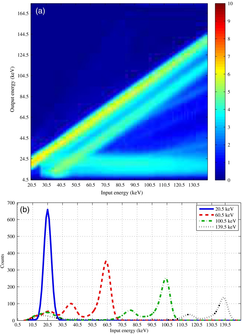
The 2-D SRF as well as 1-D profiles for several input energies is shown in Fig. 4 and was obtained as described in Sec. 3.1.2. The PCD simulation includes noise and hence, the number of counts would increase steeply at low energies (“noise floor”). The noise is currently not part of the PCD model and the SRF was modified to remove the noise floor by smoothly decreasing the counts to zero below an input energy of 14 keV.

Fig. 4.

The SRF. (a) 2-D-SRF and (b) profiles of the energy response for four different input energies.

The prominent diagonal line in Fig. 4(a) and the large peaks in Fig. 4(b) are caused by the photoelectric effect. The less prominent diagonal line and the smaller peaks are a result of K-escape photons. The bright horizontal band at low output photon energies in Fig. 4(a) is mostly caused by fluorescence photons. Charge sharing effects and Compton scatter are seen as a low-energy continuum. The energy-dependent depth-of-interaction effect affects the probability of the recorded energy and is modeled by ${\mathrm{\Omega }}_{\mathrm{SRE}}(E)$.

4.1.2. Parameters for the PPE model

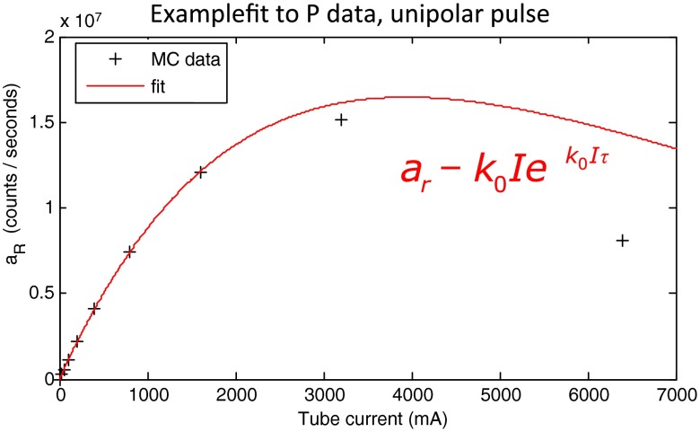
The estimated parameters ${\tau }_0$ and $k_0$ for the PPE model are listed in Table 3 for the two detection models. The count rate models were fitted to the count rates in the data above a threshold of 40 keV. The last two data points for tube currents of 3200 and 6400 mA were not used in the fit. Including this data compromised the fit quality for the lower tube currents, and these tube currents have photon rates that are much higher than one anticipates in clinical practice. It is more important to have a good agreement between data and model at lower tube currents, where the count rates are in a region that is clinically meaningful. However, the spectra at 3200 mA were included in the evaluation in order to explore the validity of our model at large count rates of up to $335\mathrm{Mcps}/{\mathrm{mm}}^2$ above 40 keV. The simulated photon fluence was identical for all data sets, and the fitted values for $k_0$ agreed within 0.8% of their mean value. An example of the count rate fit to the data is shown in Fig. 5 for the paralyzable detector.

Table 3.

Estimated parameters with standard deviations for the PPE model, averaged over pixel set $S_1$ and obtained for $E\ge 40\mathrm{keV}$.

Detector	${\tau }_0$ (ns), $E\ge 40\mathrm{keV}$	$k_0$ ($\mathrm{Mcounts}/\mathrm{s}/{\mathrm{mm}}^2/\mathrm{mA}$), $E\ge 40\mathrm{keV}$
P	$22.42\pm 0.17$	$4.12\pm 0.01$
NP	$26.91\pm 0.27$	$4.19\pm 0.02$

Fig. 5.

Count rate fit for a threshold of 40 keV as a function of the tube current to estimate the PPE model parameters. Data from the paralyzable detector are shown. Note that the last two data points at 3200 and 6400 mA were excluded from the fit.

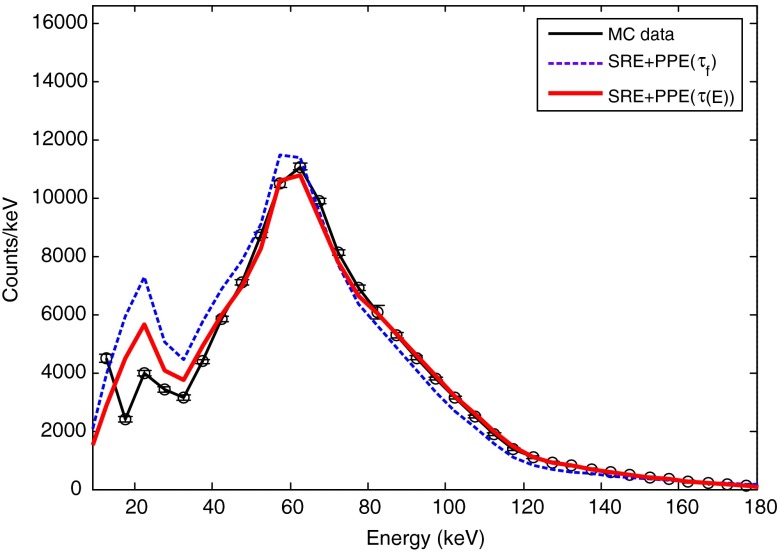
As described in Secs. 2 and 3.1.4, the spectral shape was improved by using energy-dependent dead times. The estimated parameters are listed in Table 4 for the two detector models. The spectra calculated with the energy-dependent dead time $\tau (E)$ and Eq. (11) and a fixed dead time ${\tau }_0$ and Eq. (3) are shown in Fig. 6. It can be seen that the model-data agreement was improved throughout the energy range (${\mathrm{COV}}_{\mathrm{w}}$ improved from 4.5% to 1.5%).

Table 4.

Parameters for the energy dependence of the dead time $\tau$.

Detector type	$E_0$ (keV)	${\tau }_{E_0}$ (ns)	$\kappa$ ($\mathrm{ns}/\mathrm{keV}$)
Paralyzable	20	42.0	0.15
Nonparalyzable	20	47.0	0.14

Fig. 6.

Comparison of model spectra and simulated data for the model with fixed dead time (dashed line) versus the model with energy-dependent dead time (e.g., 800 mA, paralyzable detector model).

4.2. Model-Data Agreement

This section details the data-model agreement for all data sets. The transmitted count rates $a_{\mathrm{t}}^{\prime }$ (incident onto the detector) were calculated as

$$a_{\mathrm{t}}^{\prime }=k_{0}I\times \int S_0(E)\exp (-{\int }_{\text{path}}\mu (\overrightarrow{x},E)\mathrm{d}\overrightarrow{s})\mathrm{d}E,$$ (14)

where $S_0(E)$ is the PDF of the source spectrum exiting the x-ray tube and $\mu (\overrightarrow{x},E)$ are the linear attenuation coefficients of the attenuators and the second integral is calculated along the beam path.

4.2.1. Count rate agreement

Tables 5–8 list the number of counts for one reading above an energy threshold of 40 keV for the simulated data and for the counts expected from the $\mathrm{SRE}+\mathrm{PPE}$ model. The count values were rounded to whole numbers after calculation of the relative difference.

Table 5.

Counts in data and model: P, no Gd.

Data set	Tube current (mA)	Counts in data ($868\mu \mathrm{s}$)	Counts in $\mathrm{SRE}+\mathrm{PPE}$ model ($868\mu \mathrm{s}$)	Relative difference (%)
P, no Gd	25	242	242	0.1
	50	481	482	0.1
	100	952	950	$-0.2$
	200	1861	1853	$-0.4$
	400	3554	3521	$-0.9$
	800	6453	6326	$-2.0$
	1600	10,492	9947	$-5.2$
	3200	13,118	11,259	$-14.2$

Table 8.

Counts in data and model: NP, with Gd.

Data set	Tube current (mA)	Counts in data ($868\mu \mathrm{s}$)	Counts in $\mathrm{SRE}+\mathrm{PPE}$ model ($868\mu \mathrm{s}$)	Relative difference (%)
NP, with Gd	25	154	158	2.3
	50	308	314	2.2
	100	611	625	2.4
	200	1204	1233	2.5
	400	2336	2395	2.5
	800	4399	4495	2.2
	1600	7787	7860	0.9
	3200	12,217	12,200	$-0.1$

Table 6.

Counts in data and model: P, with Gd.

Data set	Tube current (mA)	Counts in data ($868\mu \mathrm{s}$)	Counts in $\mathrm{SRE}+\mathrm{PPE}$ model ($868\mu \mathrm{s}$)	Relative difference (%)
P, with Gd	25	154	158	2.1
	50	308	315	2.3
	100	611	624	2.2
	200	1204	1229	2.1
	400	2336	2381	2.0
	800	4393	4454	1.4
	1600	7732	7667	$-0.8$
	3200	11,734	10,848	$-7.6$

Table 7.

Counts in data and model: NP, no Gd.

Data set	Tube current (mA)	Counts in data ($868\mu \mathrm{s}$)	Counts in $\mathrm{SRE}+\mathrm{PPE}$ model ($868\mu \mathrm{s}$)	Relative difference (%)
NP, no Gd	25	242	242	0.1
	50	481	481	$-0.1$
	100	951	950	$-0.1$
	200	1861	1855	$-0.3$
	400	3556	3536	$-0.6$
	800	6477	6432	$-0.7$
	1600	10,713	10,768	0.5
	3200	14,889	15,865	6.6

4.2.2. Spectral and count rate agreement

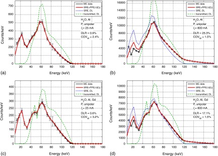
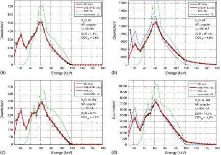
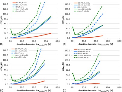
The following evaluation includes the energy-binned count rates; hence, both the count rates and the spectral shape are taken into account. Some examples of spectra are shown in Figs. 7 and 8. A graphical representation of the results can be found in Fig. 9. In all cases, the ${\mathrm{COV}}_{\mathrm{W}}$ was calculated for $E_{\mathrm{eval}}=40\mathrm{keV}$.

Fig. 7.

Data and model spectra for the paralyzable detector, without and with Gd for 25 and 800 mA.

Fig. 8.

Data and model spectra for the nonparalyzable detector, without and with Gd for 25 and 800 mA.

Fig. 9.

Graphical representation of the data-model agreements as a function of the dead time loss ratio.

4.3. Compensation of Spectral Distortions

Table 9 shows the results of the thickness estimation for the paralyzable detector model at the lowest tube current and at a tube current of 800 mA for the model spectra $n_{\mathrm{SRE}+\mathrm{PPE}},n_{\mathrm{SRE},\mathrm{DL}}$, and $n_{\mathrm{t},\mathrm{DL}}$. The evaluation of the cascaded model for the nonparalyzable detector in Sec. 4.2.2 showed similar agreement between simulated data and model as the paralyzable detector. Therefore, the thickness estimation for the nonparalyzable detector was performed only on one data set as a cross check, because similar results are expected as for the paralyzable detector. The last line in Table 9 shows that the compensation works equally well for both detector types within their statistical uncertainties.

Table 9.

Thickness estimation results. The relative bias was calculated as $(\text{estimated thickness}-\text{true thickness})/(\text{statistical uncertainty of}\text{estimated thickness})$. The statistical uncertainty was calculated from the standard deviation of measured thicknesses over all 488 simulated noise realizations.

	Estimated thicknesses			Relative bias
Model, tube current, attenuation	${\mathrm{H}}_2\mathrm{O}$ (mm)	Al (mm)	Gd (mm)	${\mathrm{H}}_2\mathrm{O}$ (std)	Al (std)	Gd (std)
Truth	100.0	3.5	0.075	—	—	—
P detector
$n_{\mathrm{SRE}+\mathrm{PPE}}(E)$, 25 mA, no Gd	$99.8\pm 6.3$	$3.5\pm 1.8$	—	$-0.03$	0.00	—
$n_{\mathrm{SRE}+\mathrm{PPE}}(E)$, 25 mA, with Gd	$98.6\pm 5.9$	$4.8\pm 2.4$	$0.068\pm 0.020$	$-0.24$	0.54	$-0.35$
$n_{\mathrm{SRE}+\mathrm{PPE}}(E)$, 800 mA, no Gd	$99.5\pm 2.3$	$2.9\pm 0.7$	—	$-0.22$	$-0.86$	—
$n_{\mathrm{SRE}+\mathrm{PPE}}(E)$, 800 mA, with Gd	$96.4\pm 1.7$	$3.1\pm 0.7$	$0.093\pm 0.004$	$-2.18$	$-0.65$	4.50
$n_{\mathrm{SRE},\mathrm{DL}}(E)$, 800 mA, no Gd	$10.0\pm 0.0$	$30.0\pm 0.0$	—	n.a.	n.a.	—
$n_{\mathrm{t},\mathrm{DL}}(E)$, 800 mA, no Gd	$113.7\pm 1.1$	$4.1\pm 0.3$	—	11.98	1.79	—
NP detector	Estimated thicknesses			Relative bias
Model, tube current, attenuation	${\mathrm{H}}_2\mathrm{O}$ (mm)	Al (mm)	Gd (mm)	${\mathrm{H}}_2\mathrm{O}$ (std)	Al (std)	Gd (std)
$n_{\mathrm{SRE}+\mathrm{PPE}}(E)$, 800 mA, no Gd	$97.8\pm 2.2$	$3.6\pm 0.7$	—	$-1.00$	0.14	—

5. Discussion

5.1. Model Evaluation

The estimation of the model parameters entails three main components: the SRF, the pulse shape, and the detector dead time. The SRF was estimated from the simulation of a single pixel and applied to all pixels in the detector (Sec. 4.1.1). This was possible because pixel-to-pixel variations were not simulated except for differences from noise and pixels near the edge of the detector were excluded from this study. The unipolar pulse shape was approximated with triangular shapes, which simplifies the calculation of the PPE (Sec. 3.1.3). The fits to the count rates as a function of tube current provided the “effective” dead times for the models, assuming a paralyzable or nonparalyzable detector model, respectively (Sec. 4.1.2). The corresponding values for the scale factor $k_0$ (Table 3), which measures the photon count rate exiting the x-ray tube, were consistent for both detector models. The comparison of the measured and expected count rates (Tables 5–8) shows agreement to better than 2.5% for tube currents up to 800 mA (which corresponds to dead time losses of up to 26%). The agreement is better than 5.8% for dead time losses up to 32%.

The simulated data spectra and the model spectra $n_{\mathrm{SRE}+\mathrm{PPE}}$ are shown in Figs. 7 and 8 for tube currents of 2 and 800 mA for the paralyzable and the nonparalyzable detector without and with Gd as attenuator. Also shown in the same figures are the spectra $n_{\mathrm{SRE},\mathrm{DL}}$ (SRE model only, scaled by dead time losses) and $n_{\mathrm{t},\mathrm{DL}}$ (no detector distortions, scaled by dead time losses). At low count rates (tube current of 25 mA), $n_{\mathrm{SRE}+\mathrm{PPE}}$ and $n_{\mathrm{SRE},\mathrm{DL}}$ are practically identical because the pulse pileup is negligible. The $\mathrm{SRE}+\mathrm{PPE}$ model captures all features of the simulated data spectra, including the dip at the K-edge in the data sets with gadolinium as additional attenuator. The agreement between data and model is ${\mathrm{COV}}_{\mathrm{W}}=3.2\%$ or better. It is obvious from the figures that the transmitted spectrum alone, neglecting the spectral distortions from SRE, cannot be used to model the data. At a tube current of 800 mA, the dead time losses reach up to 28% for some of the data sets. The effect of pulse pileup is noticeable by increased counts above 120 keV. This high energy tail is modeled by the $\mathrm{SRE}+\mathrm{PPE}$ model but is missing in the SRE-only and the transmitted spectra. The agreement between data and model is ${\mathrm{COV}}_{\mathrm{W}}=1.9\%$ or better.

Figure 9 shows the ${\mathrm{COV}}_{\mathrm{W}}$ as a function of dead time loss ratio$(DLR)=1-n_{recorded}/n_t$ for the three model spectra for tube currents between 25 and 3200 mA for all data sets. Included in these figures as dashed lines are also the results using the SRE-only spectra and the transmitted spectra if they are not scaled by the dead time losses. The data-model agreement for the full $\mathrm{SRE}+\mathrm{PPE}$ model, $n_{\mathrm{SRE}+\mathrm{PPE}}$, is ${\mathrm{COV}}_{\mathrm{W}}=20\%$ or smaller for dead time losses up to 69%. In a clinical setting, however, dead time losses larger than about 30% would typically be avoided, and the model provides accurate estimates for dead time losses in the expected clinical count rate range. In contrast, the ${\mathrm{COV}}_{\mathrm{W}}$ values for the model spectra $n_{\mathrm{SRE},\mathrm{DL}}$ and $n_{\mathrm{t},\mathrm{DL}}$ are much larger, reaching almost 100% for $n_{\mathrm{t},\mathrm{DL}}$ at a tube current of 3200 mA.

It should be emphasized that the ${\mathrm{COV}}_{\mathrm{W}}$ takes into account the agreement between data and model of both the count rates and the spectral shape. Although the threshold for the calculation of the ${\mathrm{COV}}_{\mathrm{W}}$ was set to 40 keV, a discrepancy between data and model anywhere in the spectrum would reflect in large values of the ${\mathrm{COV}}_{\mathrm{W}}$. It is of particular interest to observe in Figs. 7 and 8 that the model agrees very well with the data for energies above 120 keV at high count rates.

5.2. Compensation of Spectral Distortions

In general, the estimated attenuator thicknesses for the paralyzable detector using the spectrum $n_{\mathrm{SRE}+\mathrm{PPE}}(E)$, predicted by the cascaded $\mathrm{SRE}+\mathrm{PPE}$ model, were in agreement with the true values within one standard deviation (Table 9). Only the data at 800 mA with gadolinium resulted in a larger difference of 2.2 standard deviations for water and 4.5 standard deviations for gadolinium. The dip at the K-edge of gadolinium is somewhat more pronounced in the model than in the data, resulting in a larger bias in the thickness estimation for this data set. The estimation for the nonparalyzable detector showed similar accuracy as the paralyzable detector model and the estimated thicknesses were within one standard deviation of the true values.

Using the partial models, $n_{\mathrm{SRE},\mathrm{DL}}(E)$ or $n_{\mathrm{t},\mathrm{DL}}(E)$, for the estimation at 800 mA resulted in large deviations from the true values. In the case of $n_{\mathrm{SRE},\mathrm{DL}}(E)$, the boundaries of the search range were reached and no meaningful estimation could be obtained. These results emphasize the importance of using a complete model of spectral distortions in PCDs. Partial or inaccurate models would result in biases of the basis material thicknesses in material decomposition,¹⁷ which in turn would cause inaccurate quantitative results (e.g., for the amount of a contrast material in a region-of-interest) and introduce image artifacts.

We implemented a grid search in this study in order to show the potential of the cascaded $\mathrm{SRE}+\mathrm{PPE}$ model for spectral distortion compensation. It is desirable to develop a computationally efficient optimization algorithm, which can find the global minimum effectively.

5.3. Limitations

The study has several limitations. The estimation of the attenuator thicknesses assumed Poisson statistics for photon counts with no correlations between energy bins at all count rates. This assumption is not valid if the energy windows are correlated due to pulse pileup¹⁸ or when a photon is double-counted, e.g., at both K-escape peak and fluorescent peak. A more suitable statistical model would be to use a multivariate normal distribution and take into account the correlations in the covariance matrix. This should result in more precise estimations of the attenuator thicknesses than the simple Poisson model and in that sense our results are conservative.

The unipolar pulse shape was fitted using a triangle function for computational efficiency. The goodness of fitting was comparable to that with a bipolar pulse shape in Refs. ^{8, 12}, and ¹³; thus, the level of potential accuracy introduced by this fitting is expected to be similar to Ref. 12. The estimated energy is accurate when the count rates are low and an individual photon produces one count; however, there will be small errors when the count rates are high and pulses overlap. More specifically, underestimation is expected near the peak (near the incident energy) and the bottom (near the noise level), where the triangle function underestimates the actual pulse shape, while overestimations are expected at lower energies (i.e., $<50\%$ of the incident energy). There are other factors, such as charge trapping and polarization that may contribute to spectral distortions that are also not incorporated in the current model. Nonetheless, this study and previous studies showed that the agreement between the model and physical PCDs or MC data was good.

The noise floor (detector noise from electronic noise, Swank noise,¹⁹ etc.) is currently not part of the model. Inclusion of noise in the model requires detailed studies of the noise properties of photon counts in a pixelated detector with multiple energy thresholds and is left for a future study.

The baseline shift correction was not simulated in MC and consequently, it was not part of the model, which is consistent with previous studies.^8,12,13 If the baseline shift is pronounced, the model needs to be extended to include the baseline shift.

The SRF used to characterize the energy response of the PCD was estimated from a single pixel and applied to all other pixels. This was justified because the pixels in the simulated detector were identical and the counts differed only by statistical noise. In a real detector, the pixel-to-pixel variations can be quite large. However, it is straightforward to determine the model parameters individually and apply the model on a pixel-by-pixel basis as in Ref. 8.

Only two sets of attenuators were used. The use of more sets of material thicknesses would change both count rates and spectral shape incident onto the detector. However, it was already demonstrated in previous work⁸ that the model describes spectra with PMMA, Al, W, Sn, $\mathrm{Bi}+\mathrm{Al}$, and $\mathrm{Gd}+\text{water}$ as attenuators very well at low count rates. The model-PCD data agreement was comparable to this study with ${\mathrm{COV}}_{\mathrm{W}}$’s between 2.2% and 3.7%. In this study, two spectra were used: one with and the other without a K-edge material. The presence of a K-edge challenges the model especially in the lower energy range (20 to 50 keV). Repeated measurements in our previous study at different count rates showed that the model breaks down at higher count rates because an approximation was made that all thresholds trigger simultaneously and have the same dead time.

Equation (1) assumes that the spectra incident onto neighboring PCD pixels is identical, which means that the spill-out in the cross talk is the same as the spill-in. The assumption will hold with flat-field calibration; however, it will be violated in actual scans, where x-ray beams with different spectra and intensities may be incident onto neighboring pixels. The assumption could then result in partial volume effects in the reconstructed images (e.g., blurred edges). Therefore, the development of a cross talk model and integration with the pulse-pileup model would be of interest. The way to perform the calibration is also a challenge, as a flat-field illumination has been the standard detector calibration scheme in many cases. We shall leave it for future work.

6. Conclusions

We evaluated a cascaded model for the photon detection process in PCDs that divides the complex spectral distortions into count rate-independent SRE and count rate-dependent PPE. The model parameters were calculated from simulated calibration data. The predicted x-ray spectra were compared to those from MC simulations of a paralyzable and a nonparalyzable PCD with a unipolar pulse shape. The data-model agreement was better than ${\mathrm{COV}}_{\mathrm{W}}=2.0\%$ for dead time losses up to 28% and ${\mathrm{COV}}_{\mathrm{W}}=20\%$ or smaller for dead time losses up to 69%. We then studied the accuracy of the model when applied in a forward imaging algorithm that compensates for spectral distortions and estimates attenuator thicknesses from PCD data. The estimated thicknesses agreed with the true values within one standard deviation in most cases. When only parts of the spectral distortions were modeled by leaving out the PPE or the SRE then the data-model agreement and the estimated attenuator thicknesses deteriorated considerably. The results emphasize the importance of taking into account all spectral distortions when studying CT image formation with PCDs.

Biographies

Jochen Cammin received his PhD in particle physics from the University of Bonn, Germany, in 2004. He held academic research positions at the University of Rochester and the Johns Hopkins University. He completed a certificate in medical physics program at the University of Pennsylvania, Philadelphia, in 2015 and is currently a medical physics resident in radiation oncology at the Washington University in St. Louis. His research interests include various imaging modalities for radiation therapy.

Steffen Kappler received his diploma and PhD degrees in physics from Karlsruhe University, Germany, in 2000 and 2004, respectively. He worked as an assistant lecturer for RWTH Aachen, Germany, from 2005 to 2007. During this time, he was visiting researcher at Conseil Européen pour la Recherche Nucléaire, Switzerland, and Fermi National Accelerator Laboratory, USA. He joined SIEMENS Healthcare in 2007, where he is responsible for CT technology management. His research interests include detector physics and image reconstruction with special focus on photon-counting CT.

Thomas Weidinger received his diploma degree in physics from the University of Munich, Germany, in 2010. He wrote his PhD thesis in cooperation with the Univerity of Lübeck and Siemens Healthcare. Since 2014, he is working for Rosenberger Hochfrequenztechnik GmbH & Co. KG in the field of high-speed data communication.

Katsuyuki Taguchi received his BS and MSc degrees in mechanical engineering science from the Tokyo Institute of Technology in 1989 and 1991, respectively, and PhD in information science and electric engineering from the University of Tsukuba in 2002. He worked for Toshiba Medical Systems from 1991 to 2005 and joined the Johns Hopkins University in 2005, where he is currently an associate professor. His research interests include image reconstruction algorithms for four-dimensional cardiac CT and photon-counting CT.

References

- 1.Taguchi K., Iwanczyk J. S., “Vision 20/20: single photon counting x-ray detectors in medical imaging,” Med. Phys. 40, 100901 (2013). 10.1118/1.4820371 [DOI] [PMC free article] [PubMed] [Google Scholar]
- 2.Schlomka J. P., et al. , “Experimental feasibility of multi-energy photon-counting K-edge imaging in pre-clinical computed tomography,” Phys. Med. Biol. 53, 4031–4047 (2008). 10.1088/0031-9155/53/15/002 [DOI] [PubMed] [Google Scholar]
- 3.Shikhaliev P. M., “Energy-resolved computed tomography: first experimental results,” Phys. Med. Biol. 53, 5595–5613 (2008). 10.1088/0031-9155/53/20/002 [DOI] [PubMed] [Google Scholar]
- 4.Roessl E., Proksa R., “K-edge imaging in x-ray computed tomography using multi-bin photon counting detectors,” Phys. Med. Biol. 52, 4679–4696 (2007). 10.1088/0031-9155/52/15/020 [DOI] [PubMed] [Google Scholar]
- 5.Kappler S., et al. , “Contrast-enhancement, image noise, and dual-energy simulations for quantum-counting clinical CT,” Proc. SPIE 7622, 76223H (2010). 10.1117/12.843650 [DOI] [Google Scholar]
- 6.Kappler S., et al. , “First results from a hybrid prototype CT scanner for exploring benefits of quantum-counting in clinical CT,” Proc. SPIE 8313, 83130X (2012). 10.1117/12.911295 [DOI] [Google Scholar]
- 7.Knoll G. F., Radiation Detection and Measurement, Wiley, Hoboken, New Jersey: (2010). [Google Scholar]
- 8.Cammin J., et al. , “A cascaded model of spectral distortions due to spectral response effects and pulse pileup effects in a photon-counting x-ray detector for CT,” Med. Phys. 41, 041905 (2014). 10.1118/1.4866890 [DOI] [PMC free article] [PubMed] [Google Scholar]
- 9.Xu C., Danielsson M., Bornefalk H., “Evaluation of energy loss and charge sharing in cadmium telluride detectors for photon-counting computed tomography,” IEEE Trans. Nucl. Sci. 58, 614–625 (2011). 10.1109/TNS.2011.2122267 [DOI] [Google Scholar]
- 10.Wielopolski L., Gardner R. P., “Prediction of the pulse-height spectral distribution caused by the peak pile-up effect,” Nucl. Instrum. Methods Phys. Res. 133, 303–309 (1976). 10.1016/0029-554X(76)90623-6 [DOI] [Google Scholar]
- 11.Guerra P., Santos A., Darambara D. G., “Development of a simplified simulation model for performance characterization of a pixellated CdZnTe multimodality imaging system,” Phys. Med. Biol. 53, 1099–1113 (2008). 10.1088/0031-9155/53/4/019 [DOI] [PubMed] [Google Scholar]
- 12.Taguchi K., et al. , “An analytical model of the effects of pulse pileup on the energy spectrum recorded by energy resolved photon counting x-ray detectors,” Med. Phys. 37, 3957–3969 (2010). 10.1118/1.3429056 [DOI] [PMC free article] [PubMed] [Google Scholar]
- 13.Taguchi K., et al. , “Modeling the performance of a photon counting x-ray detector for CT: energy response and pulse pileup effects,” Med. Phys. 38, 1089–1102 (2011). 10.1118/1.3539602 [DOI] [PMC free article] [PubMed] [Google Scholar]
- 14.Kappler S., et al. , “A full-system simulation chain for computed tomography scanners,” in 2009 IEEE Nuclear Science Symp. Conf. Record (NSS/MIC ‘09), pp. 3433–3436 (2009). 10.1109/NSSMIC.2009.5401779 [DOI] [Google Scholar]
- 15.Balda M., et al. , “Lookup table-based simulation of directly-converting counting X-ray detectors for computed tomography,” in 2009 IEEE Nuclear Science Symp. Conf. Record (NSS/MIC ‘09), pp. 2588–2593 (2009). 10.1109/NSSMIC.2009.5402016 [DOI] [Google Scholar]
- 16.International Atomic Energy Agency—Nuclear Data Section, “Photon and electron interaction data,” 1997, https://www-nds.iaea.org/epdl97/ (June 2014).
- 17.Alvarez R. E., Macovski A., “Energy-selective reconstructions in X-ray computerised tomography,” Phys. Med. Biol. 21, 733–744 (1976). 10.1088/0031-9155/21/5/002 [DOI] [PubMed] [Google Scholar]
- 18.Wang A. S., et al. , “Pulse pileup statistics for energy discriminating photon counting x-ray detectors,” Med. Phys. 38, 4265–4275 (2011). 10.1118/1.3592932 [DOI] [PubMed] [Google Scholar]
- 19.Tanguay J., Kim H. K., Cunningham I. A., “The role of x-ray Swank factor in energy-resolving photon-counting imaging,” Med. Phys. 37, 6205–6211 (2010). 10.1118/1.3512794 [DOI] [PubMed] [Google Scholar]