Accurate, Automated Detection of Atrial Fibrillation in Ambulatory Recordings

Abstract

Purpose

A highly accurate, automated algorithm would facilitate cost-effective screening for asymptomatic atrial fibrillation. This study analyzed a new algorithm and compared to existing techniques.

Methods

The incremental benefit of each step in refinement of the algorithm was measured, and the algorithm was compared to other methods using the Physionet atrial fibrillation and normal sinus rhythm databases.

Results

When analyzing segments of 21 RR intervals or less, the algorithm had a significantly higher area under the receiver operating characteristic curve (AUC) than the other algorithms tested. At analysis segment sizes of up to 101 RR intervals, the algorithm continued to have a higher AUC than any of the other methods tested, although the difference from the second best other algorithm was no longer significant, with an AUC of 0.9992 with a 95% confidence interval (CI) of 0.9986–0.9998, versus 0.9986 (CI 0.9978–0.9994). With identical per-subject sensitivity, per-subject specificity of the current algorithm was superior to the other tested algorithms even at 101 RR intervals, with no false positives (CI 0.0%–0.8%) versus 5.3% false positives for the second best algorithm (CI 3.4–7.9%).

Conclusions

The described algorithm shows great promise for automated screening for atrial fibrillation by reducing false positives requiring manual review, while maintaining high sensitivity.

Introduction

Atrial fibrillation is a very common rhythm disturbance which is estimated to have affected over 5 million people in the US in 2010, and is projected to affect over 12 million by 2030[1]. It can be paroxysmal and asymptomatic[2], and if untreated, may increase the risk of stroke from 2 to 10%[3]. Screening for asymptomatic, paroxysmal atrial fibrillation requires prolonged monitoring and technician review of the recordings for presence of atrial fibrillation. High-accuracy automated algorithms for detection of atrial fibrillation would reduce the need for tedious and expensive manual review.

This article measures the incremental benefit of each step of a new method for highly-accurate automated detection of atrial fibrillation[4,5], and compares the results of the complete algorithm to several other published algorithms.

Materials and Methods

Source data

For training and testing of the algorithms, the annotated records from Physionet were used[6] (www.physionet.org). The atrial fibrillation database (www.physionet.org/physiobank/database/afdb/) was used for records of atrial fibrillation, and the normal sinus rhythm database (www.physionet.org/physiobank/database/nsrdb/) was used for normal sinus rhythm. Each database has annotations indicating regions containing the respective rhythms. Only regions that had been annotated as having the identified rhythm were used for analysis, that is, only regions identified as atrial fibrillation or normal sinus rhythm respectively. There are 25 records in the atrial fibrillation database, and 18 in the normal sinus rhythm database.

Programming

All programs, testing and graphs were created in Matlab (R2009a version 7.8.0.347, Mathworks, Inc., Natlick, Massachusetts, USA). All variations of the current algorithm were written in ANSII C and compiled as external functions for use in Matlab. All of the other algorithms were written in the Matlab programming language. The WFDB tools interface library, available from Physionet, was used to access the Physionet data from Matlab.

Description of the algorithm

Algorithms for the detection of atrial fibrillation generally fall into two categories: Those that are based on variability of the interval between QRS complexes (RR interval) and those that attempt to directly detect atrial activity. The algorithm described here falls in the former category, as it exclusively is based on the timing of the RR intervals. Additionally, methods for detection must use a group of beats or segment rather than a single beat for the analysis, and the accuracy of any technique is dependent on the size of this segment, increasing with larger sizes.

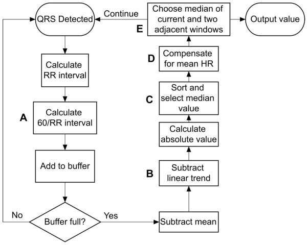
The current algorithm, called AFD for Atrial Fibrillation Detection, calculates a measure of local variability in the RR intervals within an analysis segment, and therefore the likelihood of atrial fibrillation, as illustrated in Figure 1. After a QRS complex is detected, the RR interval is computed. The RR interval is then converted to an equivalent heart rate by dividing it into 60 (Step A on Figure 1). The values are stored in a buffer until the desired number of RR intervals have been collected, called the segment width. The mean value and linear trend the values within the segment are calculated, and subtracted from each of the values (Step B). The median of the absolute value of the previous step is reported as the measure of variability for that segment (Step C). The calculated measures of variability of the preceding, current and following segment are compared, and the median value returned as the reported value for the current segment, shown in step E[4].

Fig 1.

Diagram of the steps in the algorithm. The letters denote specific steps that are key to the performance of the algorithm. See text for details

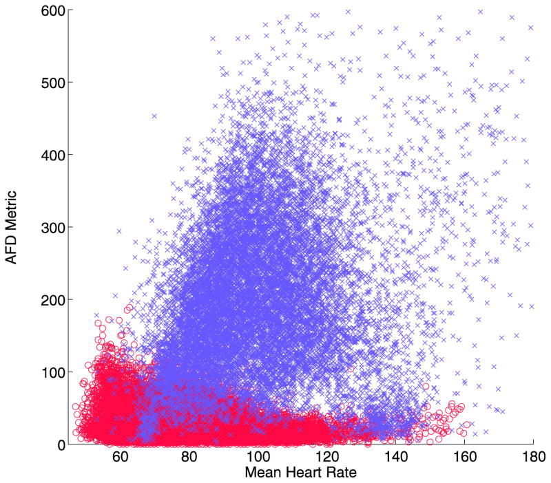
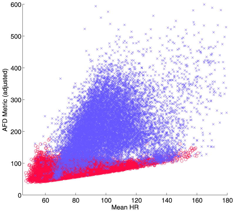
The final version of the AFD algorithm has one additional feature. Examining the output of the baseline algorithm when compared to the mean heart rate, it is apparent that there is a negative linear relationship between the calculated value and heart rate for normal sinus rhythm (Figure 2a). This means that a simple threshold will tend to have false positives at low heart rates, and false negatives at high heart rates. A linear adjustment for mean heart rate (Step D) can allow better discrimination between the two groups, when inserted before the last decision step (Figure 2b)[5].

Fig 2.

Plot of the AFD metric versus mean heart rate per analysis segment for normal sinus rhythm (o, red) and atrial fibrillation (x, lilac) in the development data set. A linear relationship is evident for the normal sinus rhythm (a), which can be adjusted linearly (b), allowing a more accurate discrimination threshold of the resulting value

Several of these steps distinguish AFD from other algorithms used to detect atrial fibrillation based on RR intervals. Each of these has been labeled with a letter in Figure 1. To test the effect of each of these distinguishing steps on the improvement in accuracy, several different versions of the algorithm lacking some of these features were used.

Statistics

The primary method for comparison of the accuracy of algorithms was the area under the receiver operating characteristic curve (AUC). The receiver operating characteristic curve is generated by plotting sensitivity as a function of (1 – specificity) while the threshold is varied through all recorded values. The AUC has a maximum value of 1.0, while for a test with no predictive value the AUC would be 0.5. The AUC was calculated using SPSS (Version 19.0.0.1, IBM, Armonk, New York, USA), which also calculated the confidence limits based on the method of Hanley and McNeil[7]. For trials using cross validation, where the AUC was calculated repeatedly, the confidence limits were calculated directly based on 1.96 x the standard error of the multiple trials.

Per-record sensitivity and specificity confidence limits were calculated based on a binomial distribution using R (Version 3.1.2, R Foundation for Statistical Computing, Vienna, Austria).

Analysis of algorithm features

To explore the impact of various steps in the algorithm on the performance, the performance was compared with versions that lacked specific steps. For this comparison, the analysis segment size was fixed at 7 RR intervals, and the AUC was used as the measure of performance.

The algorithm (AFD) was compared to versions lacking the compensation for heart rate (Step D, AFD no HR comp), lacking that and the comparison with adjacent segments (Steps D and E, AFDSingle), lacking all of those steps and the removal of the linear trend (Steps B, D and E, HR), and lacking all of these steps and using the raw RR intervals rather than the instantaneous heart rate (Steps A, B, D, and E, RR).

Comparison with other algorithms

Four other algorithms were chosen for comparison, representing a variety of strategies for detection of atrial fibrillation based on the RR intervals, as well as including the best results that have been published. These were the standard deviation of the RR interval[8] (SD), the median difference of the RR intervals[9] (Med), a Kolmogorov-Smirnov test on the histogram of differences[10,11](KS), and a wavelet -based method[12]. Of note, in a published comparison of methods by Larburu[13], the KS method was felt to have the highest specificity of all methods tested. A variable number of RR intervals was used in the analysis segments for each mentod, ranging from 5 to 101. The AUC was used as the measure of performance.

Some algorithms require training on data to adjust parameters. For this reason, each database was randomly divided into two sets of records. Six of the atrial fibrillation records (04126, 04746, 04936, 07162, 08378, 08434), and five of the normal sinus records (16273, 16786, 19090, 19140, 19830) were used for training of the algorithms tested (training set), and the remainder used for testing (test set). The records in the atrial fibrillation and normal sinus rhythm databases are about 10 and 24 hours in length respectively. For these tests, all of the algorithms were tested only on the test set, even if they did not require training.

For some of the testing situations, with longer segment sizes, the training set of atrial fibrillation records was not sufficiently large for the KS algorithm to have adequate training data. This is because the algorithm constructs 16 histograms of the RR intervals during training, each based on segments with different mean RR intervals ranging from 350 to 1100 msec. With longer segment lengths and the training records used, some of the histograms were empty since the mean RR interval required was not present in the training records. To allow comparison of that method at higher segment sizes, a 25-fold cross-validation technique was used. One of the atrial fibrillation records was selected as a test record against all 18 of the normal sinus records, and the other remaining 24 atrial fibrillation records used as a training set. After training, the discrimination of the test record from the normal sinus records was calculated. This constituted one “fold”. This procedure was then repeated for each of the atrial fibrillation records, and the results averaged.

The wavelet method required 256 RR intervals, and had two internal parameters for adjustment, so it did not lend itself to AUC analysis, and was tested separately. The parameters were adjusted for optimum performance, and the results for sensitivity and specificity compared to AFD.

Per-record specificity

In order to test the per-record specificity, a 25-fold cross-validation technique was used for training and setting of the threshold. All of the atrial fibrillation records except one were used to determine a threshold for each method, as well as training the KS method. The threshold was set as the minimum value that would label all of the training records as having at least one segment of atrial fibrillation, or 100% per-record sensitivity on the training set. This threshold was then used to analyze all of the remaining records, which included normal sinus rhythm records and the remaining atrial fibrillation record, and the count of false positive or false negative records recorded. This procedure was repeated 25 times, each time excluding a different atrial fibrillation record from the training set. The entire process was performed at an analysis segment size of 7 and 101, to test the extremes. If no episodes of atrial fibrillation in the remaining atrial fibrillation record were at least as long as the duration of the required analysis segment, that repetition was excluded from the analysis. Also, for the KS method, if the full range of mean RR intervals was not represented in the training set, that repetition was excluded. Sensitivity and specificity were reported based on the results over all the possible records and trials.

Results

Analysis of algorithm features

Table 1 shows the results of removing various features of the AFD algorithm. Each of the distinguishing features of AFD were necessary to achieve the highest discrimination, as demonstrated by the progressive reduction in the AUC with removal of each feature.

Table 1.

AUC for variants of AFD algorithm

Method	AUC	95% Confidence interval
AFD	0.9966	0.9964–0.9969
AFD no HR comp	0.9949	0.9947 – 0.9952
AFD Single	0.9845	0.9840 – 0.9850
HR	0.9751	0.9745 – 0.9758
RR	0.9192	0.9180 – 0.9204

AUC – Area under the receiver operating characteristic curve, AFD - Final algorithm, AFD no heart rate compensation (Step E removed) - AFDSingle – algorithm without voting or heart rate compensation (Steps E and D removed), HR – baseline algorithm without voting linear heart rate trend removal (Steps E, D, and B removed), RR - algorithm based on RR interval (Steps E, D, B, and A removed)

Comparison with other algorithms

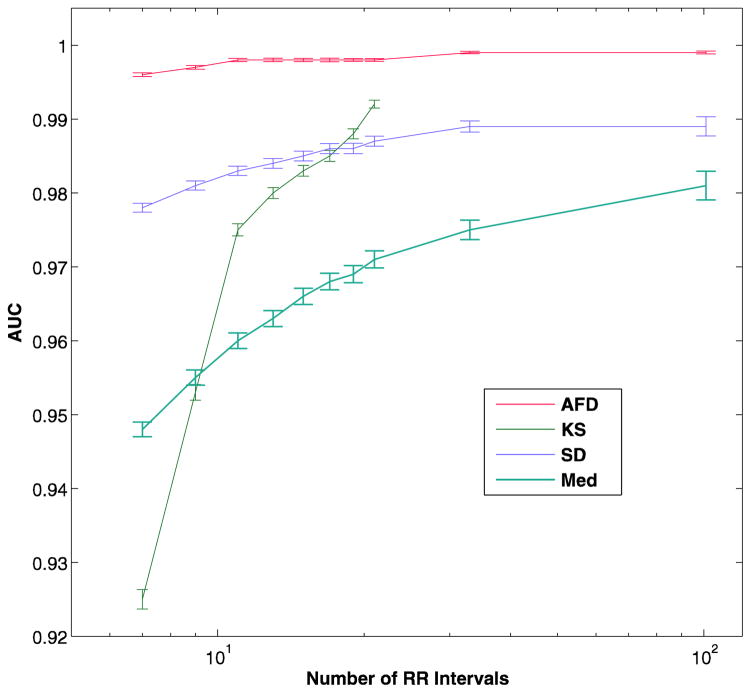
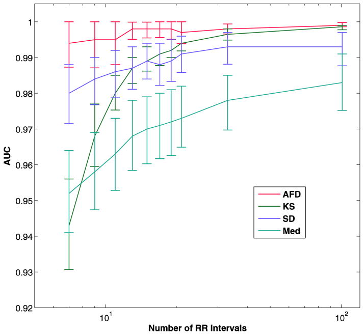
Figure 3a and in table 2 show the results of the comparison of AFD with the other algorithms, excluding the wavelet algorithm.

Fig 3.

AUC versus number of RR intervals in analysis segment in the test data set (a). The bars represent the 95% confidence intervals. The number of RR intervals is on a log scale. The panel b shows the mean AUC with 25-fold cross-validation, which allowed calculation of the KS method for large analysis segments. AFD - the current algorithm, KS - Kolmogorov-Smirnov test of the histogram of differences in RR interval, SD - standard deviation of RR intervals, Med - Median difference of the RR intervals

Table 2.

AUC for each method as a function of segment size

RR intervals	AFD (95% CI)	KS (95% CI)	SD (95% CI)	Med (95% CI)
7	0.9959 (0.9957–0.9962)	0.9245 (0.9232–0.9258)	0.9782 (0.9776–0.9788)	0.9481 (0.9471–0.9491)
15	0.9978 (0.9975–0.9980)	0.9826 (0.9819–0.9833)	0.9850 (0.9843–0.9856)	0.9658 (0.9647–0.9669)
21	0.9982 (0.9980–0.9984)	0.9923 (0.9918–0.9929)	0.9871 (0.9864–0.9878)	0.9707 (0.9695–0.9718)
33	0.9989 (0.9988–0.9991)	NA	0.9888 (0.9881–0.9896)	0.9748 (0.9735–0.9762)
101	0.9994 (0.9992–0.9996)	NA	0.9891 (0.9878–0.9904)	0.9808 (0.9788–0.9827)

AUC – Area under the receiver operating characteristic curve, AFD – current algorithm, KS – Kolmogorov-Smirnov test compared to stored template histograms, SD – standard deviation of RR intervals, Med – Median difference of adjacent RR intervals, CI – Confidence interval

The AFD algorithm had a consistently higher AUC than the other methods, and was able to maintain this higher AUC even at smaller analysis segment sizes. The KS method could not be tested at the higher analysis segment sizes of 33 and 101 because the full range of mean RR intervals was not represented in the training data set, resulting in empty histograms for some heart rate ranges. In order to compare this algorithm, which appeared to be doing better than some others at highest segment size tested (21 RR intervals), the described 25-fold cross-validation was used. The results are shown in Figure 3b and table 3.

Table 3.

AUC for each method as a function of segment size, using 25-fold cross-validation

RR intervals	AFD (95% CI)	KS (95% CI)	SD (95% CI)	Med (95% CI)
7	0.9942 (0.9873–1.0000)	0.9434 (0.9307–0.9561)	0.9797 (0.9715–0.9879)	0.9523 (0.9410–0.9636)
15	0.9977 (0.9955–0.9999)	0.9894 (0.9862–0.9926)	0.9892 (0.9840–0.9944)	0.9697 (0.9603–0.9791)
21	0.9973 (0.9939–1.0000)	0.9938 (0.9918–0.9958)	0.9908 (0.9858–0.9958)	0.9734 (0.9649–0.9819)
33	0.9980 (0.9966–0.9994)	0.9965 (0.9949–0.9981)	0.9926 (0.9881–0.9971)	0.9775 (0.9697–0.9853)
101	0.9992 (0.9986–0.9998)	0.9986 (0.9978–0.9994)	0.9925 (0.9877–0.9973)	0.9829 (0.9752–0.9906)

AUC – Area under the receiver operating characteristic curve, AFD – current algorithm, KS – Kolmogorov-Smirnov test compared to stored template histograms, SD – standard deviation of RR intervals, Med – Median difference of adjacent RR intervals, CI – Confidence interval

AFD had a significantly higher AUC at all analysis segments sizes of 19 beats or smaller than all of the other methods, with both methods of validation (p = 0.004 vs KS at 19 intervals, p < 0.0001 for all others). For the cross-validation method, although the KS method had a lower AUC than AFD at 21, 33 and 101 RR intervals, the difference was not statistically significant.

The wavelet method yielded a sensitivity of 94.5% and a specificity of 97.0% with an analysis segment size of 256 RR intervals. For comparison, selected values of sensitivity and specificity for each algorithm with a segment size of 15 are shown in Table 4. Even at this much smaller ssegment size, the AFD and KS algorithms outperform the wavelet method.

Table 4.

Specificity as a function of sensitivity for each of the tested algorithms, with a segment size of 15 RR intervals

Specificity (%)
Sensitivity (%)	AFD	KS	SD	Med
99.0	96.3	95.0	81.8	68.5
98.0	98.2	97.5	86.6	79.5
97.0	98.8	98.3	89.2	79.5
96.0	99.1	98.7	90.9	86.4
95.0	99.4	99.0	92.0	86.4
94.0	99.5	99.1	92.8	86.4
93.0	99.6	99.2	93.6	90.5
92.0	99.7	99.3	94.2	90.5

AFD – current algorithm, KS – Kolmogorov-Smirnov test compared to stored template histograms, SD – standard deviation of RR intervals, Med – Median difference of adjacent RR intervals

Per-record specificity

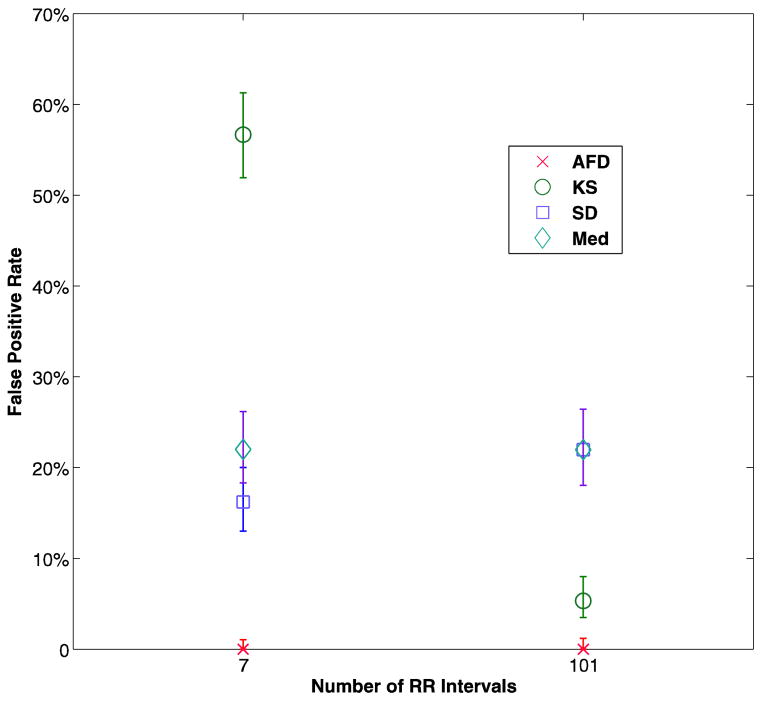
The procedure described resulted in identical sensitivity for all the methods, which was the goal. For all of the test conditions and each method, there was only one fold that resulted in a false negative result, for a sensitivity of 96% (95% CI 79.6–99.9%). The specificity results are shown in Figure 4 and table 5. There were no false positives with AFD in any of the test conditions on any of the folds, while the best results for any other method was for KS at a segment size of 101, with an average of 5.3% false positives.

Fig 4.

Average false positive records for each method, for analysis segment size of 7 RR intervals and 101 intervals. The bars represent the 95% confidence intervals. AFD - the current algorithm, KS - Kolmogorov-Smirnov test of the histogram of differences in RR interval, SD - standard deviation of RR intervals, Med - Median difference of the RR intervals

Table 5.

False positive record classifications

Method	7 RR intervals	101 RR intervals
	False Positives (95% CI)	False Positives (95% CI)
AFD	0% (0.0 – 0.8%)	0% (0.0 – 0.9%)
KS	56.7% (51.9 – 61.3%)	5.3% (3.4 – 7.9%)
SD	16.2% (12.9 – 20.0%)	22% (18.0 – 26.4%)
Med	22% (18.3 – 26.1%)	22% (18.0 – 26.4%)

AFD – current algorithm, KS – Kolmogorov-Smirnov test compared to stored template histograms, SD – standard deviation of RR intervals, Med – Median difference of adjacent RR intervals, CI – Confidence interval

Discussion

Asymptomatic, paroxysmal atrial fibrillation may require extended periods of monitoring for detection. Practical and cost effective screening would benefit from highly accurate algorithms for detection of atrial fibrillation to avoid costly and time-consuming manual review.

Numerous algorithms have been developed for the automated detection of atrial fibrillation. Most have been tested in isolation, often on proprietary databases of recordings. Larburu et al[13] compared nine different algorithms on two publicly available databases. In their test, which included the baseline version of the AFD algorithm[4] without correction for mean heart rate, they found that version of the AFD algorithm to have the highest sensitivity of all the algorithms tested, with a much shorter analysis window length. The highest specificity was obtained with the KS algorithm. Methods which incorporated analysis of the atrial activity were less robust than methods which relied exclusively on RR interval variability, and did not significantly improve accuracy. In their testing, the KS algorithm had the highest overall accuracy.

In their analysis, the method of choosing the threshold was not explained, and they reported sensitivity and specificity for a single analysis window length for each algorithm. An analysis based on AUC, as used in the current study, allows us to compare algorithms without choosing a specific threshold, and giving a single result value rather than two. As long as the receiver operating characteristic curves of two algorithms do not cross each other, the AUC gives a useful summary of the relative accuracy of the two methods.

Another issue in testing is how to define the analysis segments used. Many studies allow the segments to overlap areas of normal and abnormal rhythms, classifying the rhythm as whatever is present in > 50% of the window. This means that there are in fact three populations of segments being tested, those that are normal, those with atrial fibrillation, and a third population which has both rhythms in variable amounts, and may be classified as normal or atrial fibrillation depending on the proportion. For the current study, only segments that were entirely classified as atrial fibrillation or normal sinus rhythm were included in the analysis. This gives a clearer picture of the ability of the algorithms to discriminate the rhythms being tested. If the ability to discriminate windows with multiple rhythms is of interest, this could be the subject of a different analysis.

The AFD method of detection of atrial fibrillation incorporates several critical steps to improve discrimination. Direct use of the RR interval can lead to underdetection of atrial fibrillation at higher heart rates, since the degree of variability becomes less, a phenomenon known as pseudo-regularization. Using the reciprocal of the RR interval (Step A) reduces this problem, since smaller variations in RR interval will have a larger effect on the reciprocal if the RR is shorter. A linear change in the heart rate such as what happens with respiratory sinus arrhythmia can affect variability measures, so removing it (Step B) reduces that effect. Calculating a mean value when there is considerable variability can be inordinately influenced by the outliers, which can be mitigated by using the median value (Step C). Measures of heart rate variability may be correlated with the mean heart rate, but a compensation for this effect can be applied (Step D). Finally, the prime characteristic of the pulse during atrial fibrillation is its random nature, which can result in misclassification of a segment due to a randomly low value. The procedure in Step E reduces this problem. Comparison of the results as these features were removed shows how each contributed to achieve the best results.

The four algorithms that were chosen for comparison represent a variety of different strategies for detection, as well as including a method reported to have superior specificity and accuracy than an earlier version of the current algorithm. Comparison of the current method with the other algorithms shows that the per-segment accuracy is significantly better than all of the other algorithms at segment sizes less than or equal to 21 RR intervals. Higher numbers of RR intervals in the analysis segment caused problems with the KS algorithm training, requiring a cross-validation method of training and testing.

The cross-validation method results in a different weighting of the episodes of atrial fibrillation, since each record contributes equally, regardless of the amount of atrial fibrillation present. The number of observations is reduced as well since each recording provides only one value, increasing the variability, and therefore reducing the statistical power of the estimate. Based on this analysis, although the AUC of the AFD algorithm is higher than KS for segments sizes of 33 and 101, the difference is not significant.

All of the analyses above were based on the per-segment sensitivity and specificity. In the clinical screening application however, what is most important is the per-subject or per-record sensitivity and specificity, since this relates the probability of a subject with atrial fibrillation being detected, and how many normal studies will require manual review.

For example, if an algorithm had a 97% per-segment specificity, as does the wavelet algorithm tested, then in a 7 day recording on a normal subject we would expect 5 hours of recording to be marked as possible atrial fibrillation and require review. In the current study, a cross-validation technique was used to choose a threshold and train each of the algorithms, and then test the resulting sensitivity and specificity. The technique was designed to produce an equal sensitivity for each of the algorithms, and this was in fact observed. There was a marked difference is specificity, however. No false positives were observed with the AFD algorithm, while numerous false positives were found with all of the other techniques, with the lowest (5.3%, 95% CI 3.4–7.9%) being with the KS algorithm and segment size of 101 RR intervals.

In clinical screening of a 24 hour record, we would expect that roughly 5% of true normal records would have a false positive result with the KS algorithm, and higher numbers with the other algorithms. All of these would require manual review for correct diagnosis, adding time and cost to the screening procedure. For longer recording times of 7 days or greater, the expected false positive rate would be even higher.

A limitation of the current study is that other rhythm disturbances which could cause false positives were not included. Rhythms other than atrial fibrillation, such as frequent premature ventricular contractions or atrial contractions, or even ECG artifact, could cause additional false positives. Further testing in other databases which include additional abnormal rhythms as well as artifact would be useful to explore.

The minimal duration of atrial fibrillation that is of clinical significance has not been determined. The preferred embodiment of the KS algorithm uses a segment length of 100 RR intervals or longer, which would translate into an analysis segment potentially over 1.5 minutes long. This would reduce the ability to detect and analyze shorter episodes. The AFD algorithm preserved its high sensitivity and specificity even at smaller analysis segment sizes.

The methods differ markedly in the storage and computational requirements. This can be of importance if the algorithm is intended for implementation in a battery-powered device, with limited computational and power resources. The Med algorithm was the computationally least complex, while the SD algorithm was most complex, requiring numerous multiplications. The KS and AFD algorithms were intermediately complex, requiring addition, subtraction and sorting. The few multiplications in the AFD algorithm are all by fixed factors, and can therefore be implemented as bit-shift and addition, saving computational complexity. The KS algorithm has the greatest storage requirement, needing 16 stored histograms for different mean RR intervals, generated by the training. In addition, its performance is dependent on the particular training set that was used to create the histograms.

The novel method for automated detection of atrial fibrillation which was used has a per-subject accuracy that is significantly higher than other published algorithms, and is computationally relatively simple. It could prove useful for screening for asymptomatic atrial fibrillation.

References

- 1.Colilla S, Crow A, Petkun W, Singer DE, Simon T, Liu X. Estimates of current and future incidence and prevalence of atrial fibrillation in the U.S. Adult population. Am J Cardiol. 2013;112(8):1142–7. doi: 10.1016/j.amjcard.2013.05.063. [DOI] [PubMed] [Google Scholar]
- 2.Rho RW, Page RL. Asymptomatic atrial fibrillation. Prog Cardiovasc Dis. 2005;48(2):79–8. doi: 10.1016/j.pcad.2005.06.005. [DOI] [PubMed] [Google Scholar]
- 3.Gage BF, Waterman AD, Shannon W, Boechler M, Rich MW, Radford MJ. Validation of clinical classification schemes for predicting stroke: Results from the national registry of atrial fibrillation. JAMA. 2001;285(22):2864–70. doi: 10.1001/jama.285.22.2864. [DOI] [PubMed] [Google Scholar]
- 4.Linker DT. Long-term monitoring for detection of atrial fibrillation. 7,630,756. US Patent. 2009 Dec 8;
- 5.Linker DT. Long-term monitoring for detection of different heart rhythms. 8,326,407. US Patent. 2012 Dec 4;
- 6.Goldberger AL, Amaral LAN, Glass L, Hausdorff JM, Ivanov PCh, Mark RG, Mietus JE, Moody GB, Peng C-K, Stanley HE. PhysioBank, physiotoolkit, and physionet: Components of a new research resource for complex physiologic signals. Circulation. 2000;101(23):e215–2. doi: 10.1161/01.cir.101.23.e215. [DOI] [PubMed] [Google Scholar]
- 7.Hanley JA, McNeil BJ. The meaning and use of the area under a receiver operating characteristic (ROC) curve. Radiology. 1982 Apr;143(1):29–36. doi: 10.1148/radiology.143.1.7063747. [DOI] [PubMed] [Google Scholar]
- 8.Weisel J. Method of and apparatus for detecting atrial fibrillation. 7,020,514. US Patent. 2006 Mar 28;
- 9.Bardy H, Klein External atrial defibrillator and method for personal termination of atrial fibrillation. 7,085,601. US Patent. 2006 Aug 1;
- 10.Tateno K, Glass L. Automatic detection of atrial fibrillation using the coefficient of variation and density histograms of RR and deltarr intervals. Med Biol Eng Comput. 2001;39(6):664–7. doi: 10.1007/BF02345439. [DOI] [PubMed] [Google Scholar]
- 11.Glass L, Tateno K. Method and system for detection of cardiac arrhythmia. 7,120,485. US Patent. 2006 Oct 10;
- 12.Duverney D, Gaspoz JM, Pichot V, Roche F, Brion R, Antoniadis A, Barthélémy JC. High accuracy of automatic detection of atrial fibrillation using wavelet transform of heart rate intervals. Pacing Clin Electrophysiol. 2002;25(4 Pt 1):457–62. doi: 10.1046/j.1460-9592.2002.00457.x. [DOI] [PubMed] [Google Scholar]
- 13.Larburu N, Lopetegi T, Romero I. Comparative study of algorithms for atrial fibrillation detection. Computing in Cardiology. 2011:265–8. [Google Scholar]