

Abstract
Determining the phylogenetic relationship of two extant lineages of lobe-finned fish, coelacanths and lungfishes, and tetrapods is important for understanding the origin of tetrapods. We analyzed data sets from two previous studies along with a newly collected data set, each of which had varying numbers of species and genes and varying extent of missing sites. We found that in all the data sets the sister relationship of lungfish and tetrapods was constructed with the use of cartilaginous fish as the outgroup with a high degree of statistical support. In contrast, when ray-finned fish were used as the outgroup, which is taxonomically an immediate outgroup of lobe-finned fish and tetrapods, the sister relationship of coelacanth and tetrapods was supported most strongly, although the statistical support was weaker. Even though it is generally accepted that the closest relative is an appropriate outgroup, our analysis suggested that the large divergence of the ray-finned fish as indicated by their long branch lengths and different amino acid frequencies made them less suitable as an outgroup than cartilaginous fish.
Keywords: lungfish, phylogenomics, missing data, ray-finned fish, cartilaginous fish
Introduction
Jawed vertebrates are divided into two groups: cartilaginous fish (CF) and bony vertebrates. The latter comprise ray-finned fish (RF) and lobe-finned vertebrates (fig. 1a). Lobe-finned vertebrates, in turn, include tetrapods and lobe-finned fish. Coelacanths and lungfishes are two extant lineages of this group of fishes (fig. 1b) (Clack 2002; Benton 2005, 2015). Resolving the phylogenetic relationship of tetrapods, coelacanths, and lungfishes is important for understanding the origin of tetrapods and revealing the process of transition of vertebrates from water to land. The traditional view is that coelacanths are a sister group of tetrapods (Romer 1966) (Tree 2, fig. 1b). Recent paleontological studies favor the lungfish–tetrapod sister relationship (Tree 1, fig. 1b) (Zhu et al. 2001; Clack 2002; Zhu and Yu 2002; Zhu et al. 2006, 2009; Swartz 2009; Benton 2015). However, morphological studies have supported each of the three possible relationships of the three lineages including the sister relationship of lungfishes and coelacanths (Tree 3, fig. 1b), and this relationship is still controversial (Schultze and Trueb 1991; Clack 2002; Benton 2015).
Fig. 1.—
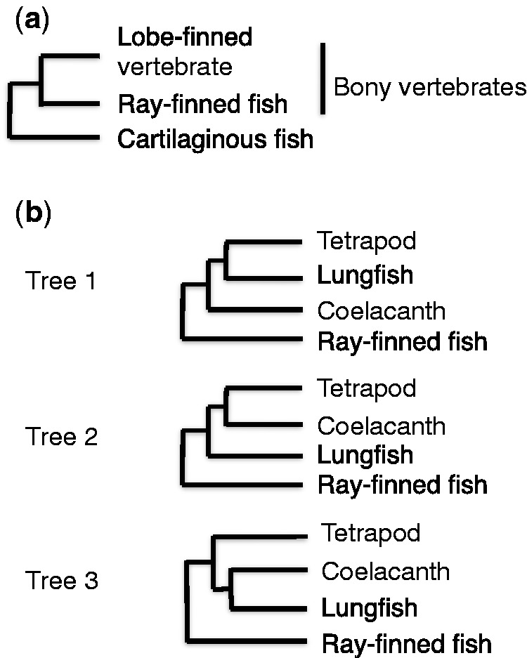
The phylogenetic relationship of the major lineages in jawed vertebrates and lobe-finned vertebrates. (a) The relationship of major lineages in jawed vertebrates. (b) Three possible relationships for the three extant lineages of lobe-finned vertebrates: Sister relationships of lungfishes and tetrapods (Tree 1), coelacanths and tetrapods (Tree 2), and lungfishes and coelacanths (Tree 3).
Molecular phylogenetic studies have also generated all three relationships (Gorr et al. 1991; Zardoya et al. 1998; Venkatesh et al. 2001; Brinkmann et al. 2004). The result was equivocal even with the use of 44 nuclear genes (Takezaki et al. 2004). However, recently, owing to sequencing of the coelacanth genome (Amemiya et al. 2013; Nikaido et al. 2013), two studies (Amemiya et al. 2013 [100,583 amino acid sites from 251 genes from 22 species]; Liang et al. 2013 [690,838 amino acid sites from 1,290 genes from 10 species]) reconstructed the sister relationship of lungfish and tetrapods with high statistical support.
Phylogenomics has become a popular approach for revealing evolutionary relationships. Although the use of a large amount of data is effective in reducing sampling error in the estimation of phylogeny, gathering genomic data from many species has its own problems (Philippe et al. 2005). The effects of missing data in sequence alignments because of varying quality among genome sequences and the loss of genes in specific lineages are not well understood (Philippe et al. 2011). Combining information from many genes that have been subjected to heterogeneous evolutionary processes by concatenation of gene sequences may generate errors (Nishihara et al. 2007; Hess and Goldman 2011). Furthermore, there may be factors to give systematic biases to phylogeny construction such as different nucleotide/amino acid compositions or heterotachious change among species/taxonomic groups (Phillips et al. 2004; Rodriguez-Ezpeleta et al. 2007). Therefore, even with the phylogenomic approach, careful consideration is necessary in taxon sampling and the choice of tree-making methods and substitution models.
In this study, to evaluate these effects and potential errors in the phylogenomic analysis of coelacanth, lungfish, and tetrapods, we analyzed the data sets used by the previous two studies and our newly collected data (242,475 amino acid sites from 831 genes from 26 species).
Materials and Methods
RNA Extraction of Lungfish and Transcriptome Analysis
A right pectoral fin and pelvic fin were dissected from a lungfish (Protopterus dolloi) and used for RNA extraction. The tissues were individually homogenized in TRIzol reagent (Life Technologies, Inc.), and RNAs were extracted with TRIzol according to the manufacturer's procedure. The RNA samples were used to construct individual paired-end libraries with ∼200-bp inserts followed by sequencing using the Illumina HiSeq 2000 at Beijing Genomics Institute (Shenzhen, China). Over 4.4 Gb of paired-end 100-bp reads were generated from each sample. Low-quality bases were trimmed using the DynamicTrim program in SolexaQA (Cox et al. 2010) with a Phred quality score cutoff of 20. All the reads were used for de novo transcriptome assembling with Trinity (Grabherr et al. 2011), and putative coding sequences were extracted using TransDecoder (http://transdecoder.github.io/). Finally, a total of 23,485 open reading frame sequences with ≥450 bp was obtained. The lungfish sequence reads were deposited in NCBI Sequence Read Archive under the accession numbers SRX895335 and SRX895362.
Sequence Data of 25 Vertebrate Species
RNA-seq data from little skate (Leucoraja erinacea), spotted catshark (Scyliorhinus canicula), and elephant shark (Callorhinchus milii) were retrieved from NCBI (accession numbers SRX036536–SRX036538), and coding sequence assemblies were generated according to the procedure described above. For the three sharks, 28,856, 25,650, and 27,829 open reading frame sequences of ≥300 bp were generated, respectively.cDNA data were downloaded from Ensembl release 76 (Cunningham et al. 2015) for human (Homo sapiens), mouse (Mus musculus), dog (Canis lupus familiaris), armadillo (Dasypus novemcinctus), elephant (Loxodonta africana), opossum (Monodelphis domestica), Tasmanian devil (Sarcophilus harrisii), turkey (Meleagris gallopavo), chicken (Gallus gallus), duck (Anas platyrhynchos), flycatcher (Ficedula albicollis), turtle (Pelodiscus sinensis), lizard (Anolis carolinensis), western clawed frog (Xenopus tropicalis), coelacanth (Latimeria chalumnae), zebrafish (Danio rerio), medaka (Oryzias latipes), platyfish (Xiphophorus maculatus), tilapia (Oreochromis niloticus), stickleback (Gasterosteus aculeatus), pufferfish (Takifugu rubripes), and cod (Gadus morhua).
Collection of Orthologs from 26 Species
First, we obtained orthologs for lungfish, shark, and human genes. A BLAST search was done with the lungfish genes as the query sequences against data from each of the three shark species and the human data. With the best-hit genes from the sharks and human as queries, the search was done against the human data and the shark data, respectively. If the human and shark genes were reciprocal best hits, they were considered as orthologs of the lungfish gene used as the first query. Similarly, coelacanth orthologs were obtained by the BLAST search, using the lungfish genes as queries against the coelacanth data and the human data. In this case, if the best-hit genes of coelacanth and human were annotated as 1-to-1 orthologs in Ensembl, we considered them as orthologs of the lungfish gene of the query.
In these BLAST searches, we used the lungfish data as the queries because insufficient transcriptome coverage might prevent the finding of orthologs. We used the human data as a search database to anchor the ortholog search. Nucleotide BLAST (r = 2, G = 2, E = 2, e-value cutoff of 1 × 10⁻¹⁰) was used in all the searches because protein BLAST is likely to give a false hit for paralogous genes sharing the same amino acid domain because of high sequence similarity.
Orthologs of the 13 nonhuman tetrapods and zebrafish were collected according to 1-to-1 ortholog annotation with human genes in Ensembl, and orthologs of teleost fish except for zebrafish according to the 1-to-1 ortholog annotation with zebrafish genes. The collected ortholog data were translated to amino acid sequences and aligned using MAFFT (Katoh and Standley 2013) with highly accurate settings of –maxiterate 1000 and –localpair. All the alignments were visually checked, and obviously misaligned regions such as those including highly variable positions and species-specific splice variants were excluded. Ambiguous sites and gap-containing sites were also excluded. Genes of short length (<100 amino acids) were discarded. Finally, 831 genes with 242,475 ungapped amino acid positions were obtained for the 26 species (data set III).
Sequence Data from Previous Studies
The data from two previous studies were provided by the authors upon our request. Data from Amemiya et al. consisted of concatenated sequences from 20 species with 112,212 amino acid sites (table 1) (data set I). Compared with the data for 22 vertebrates with 100,583 amino acid sites described in Amemiya et al. (2013), 2 CFs (spotted catshark and elephant shark) were missing and the number of included amino acid positions was slightly larger.
Table 1.
Data Sets Analyzed in this Study
| Data Set | Source | Genes | Amino Acid Sites | Species | Missing Sites (%) |
|---|---|---|---|---|---|
| I | Amemiya et al. | 251 | 112,212 | 20 | 14.2 |
| II | Liang et al. | 1,288 | 618,946 | 10 | 6.5 |
| III | This study | 831 | 242,475 | 25 | 0 |
Note.—In data set I, only concatenated sequence was available, and two shark species were missing. In data set II, genes with <50 amino acid sites were excluded.
Sequence data provided by Liang et al. consisted of alignments of 1,465 individual genes. We used alignments of 1,288 genes with ≥50 shared sites for the 10 species (table 1) (data set II). This data set was slightly smaller than that of Liang et al. (2013), which consisted of 1,290 genes and a total of 690,838 amino acid sites and 351,095 shared sites (table S4 in Liang et al. 2013). Differences in the genes used for this data set are shown in supplementary table S1, Supplementary Material online.
Missing Data
In data set I, the percentage of missing sites ranged from 0.2% (human) to 92.9% (Chinese brown frog, Rana chensinensis) with an average of 14.2% (table 1 and supplementary table S2, Supplementary Material online), and there were 1,374 shared sites across all species. In data set II, within the total of 618,946 amino acid sites, 370,750 sites were shared across all 10 species. The percentages of missing sites ranged from 1.7% (human) to 22.0% (lungfish), with an average of 6.5% (table 1 and supplementary table S2, Supplementary Material online). Because the missing data may affect the accuracy of phylogeny construction (e.g., Roure et al. 2012; Jiang et al. 2014; and references therein), we constructed phylogenetic trees by excluding the five species with the highest percentages of missing data (armadillo 47.8%; tammar wallaby [Macropus eugenii] 45.1%; platypus [Ornithorhynchus anatinus] 31.3%; turkey 10.7%; Chinese brown frog 92%) in Amemiya et al.’s data and using only the shared sites in Liang et al.’s data. After excluding the 5 sequences with the high percentage of missing data in data set I, there were 66,928 shared sites and the average proportion of missing data was 3.7%. However, the tree topologies and the statistical support were essentially the same as for analyses using the whole data sets. Therefore, we decided to show only the results using all the species and all the sites.
Data Sets Consisting of Longest 20% of Genes
We prepared data sets consisting of the upper 20% of genes based on their length for data sets II and III (P20L). The P20L data sets consisted of about half of the total number of amino acid sites, and the average number of sites per gene was about two times larger than that for each of the whole data sets (supplementary table S3, Supplementary Material online).
Phylogenetic Analyses
Maximum-Likelihood Method
Phylogenetic trees were constructed by the maximum-likelihood (ML) method using PhyML 3.1 (Guindon et al. 2010). We compared the likelihood values using four empirical substitution models, JTT (Jones et al. 1992), LG (Le and Gascuel 2008), WAG (Whelan and Goldman 2001), and Dayhoff (Dayhoff et al. 1978) models, for concatenated sequences and individual genes, whether or not rate heterogeneity was assumed across sites (G4, discrete gamma distribution with four categories and G8 with eight categories) and invariant sites (I) were assumed, or amino acid frequencies (F) were estimated from the data (supplementary tables S4 and S5, Supplementary Material online). Among the four substitution models, the JTT model had the highest likelihood values. The increases in likelihood values with the settings of I and G8 were relatively small in comparison with the increases with the settings of G4 and F and the constructed tree topologies for concatenated sequences did not change. Therefore we decided to use JTTFG4 in the ML analysis.
ML trees for concatenated sequences were also constructed using RAxML 8.1.16 (Stamatakis 2014) with JTTFG4 and GTR (general time reversible) + G4 models. The likelihood and bootstrap values of the trees generated with JTTFG4 were similar to those generated by PhyML. Therefore, we show only the result of GTRG4 by RAxML. For the bootstrap tests, 500 replications were carried out.
In addition to the search of the best trees, likelihoods were computed for the possible tree topologies with the known taxonomic relationships fixed and ambiguous relationships taken into account (supplementary table S6, Supplementary Material online). For data set II, the likelihood values were computed for three tree topologies that correspond to Trees 1, 2, and 3 (fig. 1b), whereas the other parts of the tree remained fixed (fig. 2b). For data set I, the relationships of elephant, armadillo, and other eutherian mammals were not established (U1, U2, and U3 in supplementary table S6, Supplementary Material online). Therefore, likelihoods were computed for the nine possible tree topologies by taking these ambiguous relationships into account. For data set III, in addition to the relationships of elephant, armadillo, and other eutherian mammals, by using different tree construction methods and assuming substitution patterns, stickleback came closer to the cluster of tilapia, platyfish, and medaka than pufferfish (V1), or pufferfish and stickleback formed a monophyletic group (V2). Therefore, likelihoods were computed for 18 possible tree topologies when the RF was included. The AU test in CONSEL (Shimodaira and Hasegawa 2001) was carried out for the likelihoods computed for the possible tree topologies.
Fig. 2.—

Maximum-likelihood trees constructed for concatenated sequences of the three data sets. (a)–(c) CF and RF were used as the outgroup. (d)–(f) RF was used as the outgroup. (a) and (d) Data set I from Amemiya et al. (2013). (b) and (e) Data set II from Liang et al. (2013). (c) and (f) Data set III collected in this study. The numbers on the branches are BPs from 500 replications. The trees were constructed with the JTTFG4 setting by PhyML.
Multispecies Coalescent-based Method
We estimated species phylogeny by the multispecies coalescent-based (MSC) method using ASTRAL 4.7.12 (Mirarab et al. 2014). Using ML trees of individual genes with the setting of JTTFG4, statistical support was evaluated by the multilocus bootstrap approach (Seo 2008) with 500 replications. An exact search of quartet trees was carried out for data set II and a heuristic search was done for data set III.
Bayesian Method
Bayesian trees were generated using MrBayes 3.2.2 (Altekar et al. 2004) with settings of JTTFG4 and GTRG4. Two simultaneous runs were carried out. The number of generations was set to 500,000 for data sets I and III; 200,000 for data set II in the case of JTTFG4; and 8,000,000, 2,400,000, and 4,000,000 for data sets I, II, and III, respectively, in the case of GTRG4. The burn-in fraction was set to 0.2 for JTTFG4 and 0.5 for GTRG4. We used the default values for all other settings. We also generated trees with the setting “mixed,” in which ten empirical substitution models including JTT, WAG, and Dayhoff are sampled and averaged, together with the setting G4. Because the results were essentially the same as those from JTTFG4 (data not shown), we showed only the results from JTTFG4.
In our preliminary study, we tried the CAT model with G4 in PhyloBayes 3.3f (Lartillot et al. 2009). However, it was taking a prohibitive amount of time and we could not obtain sufficient convergence. Therefore we did not use the CAT model in this study.
Determination of the Phylogenetic Network
Network trees were constructed using the neighbor-net with JTT + G distance, and δ scores (Holland et al. 2002) were calculated by SplitsTree 4.14.2 (Huson and Bryant 2006).
Exclusion of Variable Positions
The number of substitutions per site was computed by parsimony using PROTPARS in PHYLIP 3.6 (Felsenstein 2005) for all the possible tree topologies and the average was taken (supplementary table S7, Supplementary Material online). In total, 5%, 10%, and 20% of highly variable sites were excluded to reduce the effect of long branch attraction (Brinkmann and Philippe 1999). The excluded sites were those with ≥4, 6, and 8 substitutions for data set I; ≥6, 7, and 9 substitutions for data set II; and ≥4, 7, and 9 substitutions for data set III. However, the tree topologies did not change.
Computer Simulation
Sequences of 300 amino acids for the 5 taxa (tetrapod, coelacanth, lungfish, RF, CF) were generated by Seq-Gen (Rambaut and Grassly 1997), assuming Tree 1–3 topologies and estimated values of branch lengths and gamma parameters with the setting JTTG for data sets I, II, and III. One thousand replications were carried out. For each set of the five sequences, ML trees were constructed by PhyML with JTTFG4 using CF + RF, RF, and CF as the outgroup in each replication. Likelihood was computed for the three possible topologies corresponding to Trees 1–3, and the number of replications in which the topology with the highest likelihood was counted. If two or three topologies had the same highest likelihood value (tie case), a value of 1/2 or 1/3 was counted up for those topologies, depending on the number of the tie tree topologies generated.
Results
ML Trees Constructed from Concatenated Sequences
In this study, we analyzed three data sets (I–III), in which the number of genes, the number of species, and the percentage of missing sites varied (table 1). Figure 2 shows ML trees constructed for concatenated sequences of all genes from the three data sets: Data from Amemiya et al. (2013) (data set I), data from Liang et al. (2013) (data set II), and data collected in this study (data set III). The JTT model with rate heterogeneity across sites following the gamma distribution was assumed, and amino acid frequencies were estimated from data used (JTTFG4) (see Materials and Methods). When the CF and RF (CF + RF) were used as the outgroup, as in Amemiya et al. (2013) and Liang et al. (2013), the sister relationship of lungfish and tetrapods (Tree 1 in fig. 1b) was reconstructed with high bootstrap probabilities (BPs) for all the data sets (87%, 100%, and 100% for data set I, II, and III, respectively) (fig. 2a–c). However, when only RF was used as the outgroup, coelacanth became a sister to tetrapods in all the data sets (Tree 2 in fig. 1b), although the BP was significantly high only for data set II (95%) and was low for data sets I and III (54% and 52%, respectively) (fig. 2d–f). By using only CF as the outgroup, Tree 1 was reconstructed for all three data sets with similar or slightly higher BPs (97%, 100%, and 99% for data sets I, II, and III, respectively) (supplementary fig. S1, Supplementary Material online) as compared with those using CF + RF as the outgroup.
Likelihoods computed for the possible tree topologies and the results from the AU tests were consistent with the constructed trees (table 2 and supplementary table S8, Supplementary Material online). When the outgroup was CF + RF or CF, as the best trees searched mentioned above, tree topologies with Tree 1 (Tree 1 topologies) had the highest likelihood values. Tree 2 and Tree 3 topologies were rejected by the AU test for data sets II and III (P ≤ 0.001) and for data set I with CF as the outgroup (P < 0.05). Tree 3 topology was not rejected for data set I when CF + RF was the outgroup (P = 0.146). This corresponds to the nonsignificant BP value supporting Tree 1 (87%) in this case. When RF was the outgroup, Tree 2 topologies had the highest likelihood values for all three data sets. For data set II, consistent with the high BP that supported Tree 2, Tree 1 and Tree 3 topologies were rejected (P ≤ 0.001), and for data sets I and III, in addition to Tree 2 topologies, both Tree 1 and Tree 3 topologies were not rejected by the AU test (P > 0.07). However, the P-value for the AU test was relatively high for Tree 3 (P = 0.57) and low for Tree 1 (P = 0.09) for data set I, whereas the P-value for Tree 1 was relatively high (P = 0.68) and that of Tree 3 was low (P = 0.07) for data set III. As in the case with JTTFG4, ML trees with the GTR model (GTRG4) were Tree 1 supported by high BPs (≥89% for data set I and 100% for data sets II and III) when CF + RF or CF was the outgroup (supplementary fig. S2, Supplementary Material online, and table 3). When RF was the outgroup, although Tree 2 was generated for all the data sets with JTTFG4, Tree 3 and Tree 1 were generated with GTRG4 for data sets I and III, respectively. However, the BPs were low (≤59%) with both GTRG4 and JTTFG4.
Table 2.
Log-Likelihood Values of Concatenated Sequences
| Data Set | Tree | Outgroup |
||||||||
|---|---|---|---|---|---|---|---|---|---|---|
| CF + RF |
CF |
RF |
||||||||
| ΔL/L | AU | ΔL/L | AU | ΔL/L | AU | |||||
| I | 1 | −1,241,832.7 | Best | 0.738 | −1,016,570.7 | Best | 0.624 | −56.8 | 0.094 | |
| 2 | −82.6 | 0.028 | −80.8 | 0.044 | −1,157,666.6 | Best | 0.621 | |||
| 3 | −53.6 | 0.146 | −134.5 | 1 × 10⁻⁵ | −3.1 | 0.574 | ||||
| II | 1 | −5,726,397.0 | Best | 1 | −4,779,270.5 | Best | 1 | −278.3 | 0.001 | |
| 2 | −593.6 | 2 × 10⁻⁵ | −404.9 | 8 × 10⁻⁶ | −5,243,076.5 | Best | 0.936 | |||
| 3 | −503.2 | 1 × 10⁻³⁵ | −697.3 | 7 × 10⁻⁵ | −121.6 | 0.001 | ||||
| III | 1 | −3,086,859.0 | Best | 0.855 | −2,296,640.0 | Best | 0.832 | −5.0 | 0.680 | |
| 2 | −308.3 | 5 × 10⁻⁶ | −224.9 | 0.001 | −2,715,213.2 | Best | 0.765 | |||
| 3 | −270.7 | 3 × 10⁻⁴ | −415.2 | 6 × 10⁻⁵ | −103.2 | 0.073 | ||||
Note.—“AU” refers to the P-value from the AU test; JTTFG4 was assumed. Tree topologies for data sets I and III take into account the ambiguities in relationship of elephant, armadillo, and the other eutherian mammals, and those for data set III the ambiguities in pufferfish and stickleback and the cluster of tilapia, platyfish, and medaka (supplementary table S6, Supplementary Material online). The results for the topologies with the highest likelihood value among those with Trees 1, 2, and 3 are shown; the results of all tree topologies are shown in supplementary table S8, Supplementary Material online. L = log-likelihood for the best tree. ΔL = the difference in the log-likelihood values relative to the best tree.
Table 3.
Summary of Tree Topologies and their Statistical Support
| Data Set | Method | Substitution Model | Outgroup |
|||||
|---|---|---|---|---|---|---|---|---|
| CF + RF |
CF |
RF |
||||||
| Tree | BP or PP | Tree | BP or PP | Tree | BP or PP | |||
| I | ML | JTTFG4 | 1 | 87 | 1 | 97 | 2 | 54 |
| GTRG4 | 1 | 89 | 1 | 100 | 3 | 51 | ||
| Bayesian | JTTFG4 | 1 | 1.00 | 1 | 1.00 | 2 | 1.00 | |
| GTRG4 | 1 | 1.00 | 1 | 1.00 | 3 | 1.00 | ||
| II | ML | JTTFG4 | 1 | 100 | 1 | 100 | 2 | 95 |
| GTRG4 | 1 | 100 | 1 | 100 | 2 | 88 | ||
| Bayesian | JTTFG4 | 1 | 1.00 | 1 | 1.00 | 2 | 1.00 | |
| GTRG4 | 1 | 1.00 | 1 | 1.00 | 2 | 1.00 | ||
| MSC | JTTFG4 | 1 | 100 | 1 | 99.8 | 2 | 83.3 | |
| 3 | 15.8 | |||||||
| III | ML | JTTFG4 | 1 | 100 | 1 | 97 | 2 | 52 |
| GTRG4 | 1 | 100 | 1 | 100 | 1 | 59 | ||
| Bayesian | JTTFG4 | 1 | 1.00 | 1 | 1.00 | 2 | 1.00 | |
| GTRG4 | 1 | 1.00 | 1 | 1.00 | 1 | 1.00 | ||
| MSC | JTTFG4 | 1 | 99.4 | 1 | 98.4 | 2 | 48.1 | |
Note.—BP: bootstrap probability (for ML and MSC methods). PP: posterior probability (for Bayesian analyses).
ML Analyses of Individual Genes
We computed likelihood values for individual genes in data sets II and III for the possible tree topologies using JTTFG4. Consistent with the ML trees constructed from the concatenated sequences, the largest numbers of genes supported Tree 1 for both data sets II and III when CF + RF or CF was the outgroup, and the number of genes that supported the Trees 1, 2, or 3 differed significantly (P < 0.02 by chi-square test) (table 4). In contrast, when RF was the outgroup, the largest number of genes supported Tree 3 in data set II and Tree 2 in data set III, but the differences in the number of genes that supported Trees 1, 2, or 3 became small (P = 0.98 for data set II and 0.04 for data set III by chi-square test).
Table 4.
Number of Genes that Supported Trees 1, 2, and 3
| Data Set | Tree | Outgroup |
||
|---|---|---|---|---|
| CF + RF | CF | RF | ||
| II | 1 | 517 | 522 | 429 |
| 2 | 342 | 401 | 425 | |
| 3 | 429 | 365 | 434 | |
| P value | 0.0001 | 0.0005 | 0.9767 | |
| III | 1 | 335 | 326 | 278 |
| 2 | 229 | 273 | 319 | |
| 3 | 267 | 232 | 234 | |
| P value | 0.006 | 0.0157 | 0.0373 | |
Note.—“P value” indicates that from a chi-square test.
Multispecies Coalescent-based Method
The phylogenetic trees were estimated by the MSC method (Mirarab et al. 2014) for data sets II and III (table 3). This method also generated Tree 1 with CF + RF or CF as the outgroup and Tree 2 with RF as the outgroup for both data sets. BPs in the former case (≥98.4%) were as high as those by the ML method (97%). With RF as the outgroup, BPs (83.3% for data set II and 48.1% for data set III) were slightly smaller than those from the ML method (≥88% for data set II and ≥52% for data set III). It should be noted that BP support was 15.8% for Tree 3 and was virtually zero for Tree 1 with RF as the outgroup for data set II.
Bayesian Analyses
The tree topologies generated by the Bayesian method were essentially the same as those generated by the ML method if the same substitution model was assumed (supplementary fig. S3, Supplementary Material online, and table 3). However, posterior probabilities (PPs) supporting the relationships of coelacanth, lungfish, and tetrapods were always high (1.00) even when BPs from the ML method were low (51–59%) for data sets I and III with RF as the outgroup. This is consistent with previous studies in that PPs tend to provide overconfidence (see Discussion).
Network Phylogeny
Figure 3 shows the network trees constructed for the three data sets. There are incompatibilities in the tree topologies for the common ancestral branches of tetrapods, lobe-finned fish, RF, and CF in all the data sets. In the case of data sets I and III, the network trees show incompatibilities in the common ancestors of eutherian mammals. The δ scores, which are a measure of an extent of incompatibilities in tree topologies (Holland et al. 2002), are relatively high for coelacanth and lungfish in all the data sets (supplementary table S9, Supplementary Material online). Most of the internal branches show signs of reticulation, but a Φ test for detecting recombination (Bruen et al. 2006) was significant only for data set III (P = 0.0 and P = 1.0 for data sets I and II).
Fig. 3.—
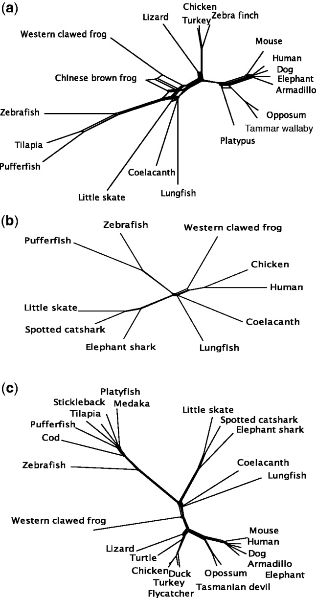
Network trees. (a) Data set I. (b) Data set II. (c) Data set III. The neighbor-net with JTTG distance was used.
Data Sets Consisting of Upper 20% of Long Genes
Because shorter genes are likely to be affected by the effect of sampling errors and their use may generate errors in phylogeny estimation, we compiled data sets consisting of the upper 20% of genes based on length (P20L) for data sets II and III (supplementary table S3, Supplementary Material online). The results were generally similar to those of the whole data sets (supplementary tables S8 and S10, Supplementary Material online) except that Tree 1 was generated by all the methods with RF as the outgroup for data set III. However, in this case BPs supporting Tree 1 were not high (≤84% by the ML method and 63.6% by the MSC method) (supplementary table S10, Supplementary Material online) and the AU test did not reject Tree 2 topologies in addition to Tree 1 topologies (supplementary table S8, Supplementary Material online). Furthermore, the largest number of genes supported Tree 2 with RF as the outgroup (supplementary table S11, Supplementary Material online). The network trees were similar to those for the whole data sets (supplementary fig. S4, Supplementary Material online), but the δ scores were slightly smaller (supplementary table S9, Supplementary Material online).
Extent of Divergence of Cartilaginous Fish and Ray-Finned Fish
Whether concatenated sequences were used or separated analysis of individual genes was carried out, the ML method consistently constructed Tree 1 with high statistical support when CF + RF or CF was used as the outgroup. In contrast, when RF was the outgroup, Tree 2 and Tree 3 were generated for data sets I and II and Tree 1 and Tree 2 were generated for data set III, although BPs were low for data sets I and III (BP ≤ 59%). The P20L data sets generated results that were consistent with those for the whole data sets.
How can we reconcile the varying results using different outgroups? As RF is taxonomically an immediate outgroup of lobe-finned fish and tetrapods, they may be more appropriate as the outgroup than CF. To determine whether CF or RF is more appropriate as the outgroup, we examined the extent of divergence of CF and RF. Supplementary figure S5, Supplementary Material online, shows Tree 1, 2, and 3 topologies of the five taxa (tetrapods, lungfish, coelacanth, RF, and CF). The estimated branch lengths were similar for all three data sets and the three tree topologies (table 5). The branch lengths for RF (0.28–0.29) were the longest and were 35–49% longer than those for CF (0.20–0.21). Note that branch lengths for tetrapods (0.18–0.21) were similar to those for CF; relative to the tetrapod branch lengths, branch lengths for lungfish (0.15–0.17) and coelacanth (0.11–0.14) were slightly shorter. The lungfish branch was longer than the coelacanth branch (17–18% in data set II and 33–38% in data sets I and III). This is consistent with the previous observation that the evolutionary rate of coelacanth was markedly slow compared with lungfish (Higasa et al. 2012; Amemiya et al. 2013; Nikaido et al. 2013). The lengths of the internal branches connecting lungfish and coelacanth (b1) were 0.01 or slightly shorter. These were a half to one-third of the branch lengths connecting CF and RF (b2).
Table 5.
Average Branch Lengths of Trees of the Five Taxonomic Groups
| Tree | Data Set | Tetrapod | Lungfish | Coelacanth | RF | CF | b1 | b2 | r1 | r2 |
|---|---|---|---|---|---|---|---|---|---|---|
| 1 | I | 0.211 | 0.162 | 0.119 | 0.284 | 0.209 | 0.009 | 0.020 | 1.37 | 1.36 |
| II | 0.205 | 0.171 | 0.146 | 0.291 | 0.207 | 0.010 | 0.018 | 1.17 | 1.40 | |
| III | 0.177 | 0.153 | 0.114 | 0.292 | 0.196 | 0.009 | 0.017 | 1.34 | 1.49 | |
| 2 | I | 0.213 | 0.161 | 0.120 | 0.283 | 0.209 | 0.008 | 0.019 | 1.34 | 1.35 |
| II | 0.208 | 0.172 | 0.147 | 0.291 | 0.207 | 0.007 | 0.018 | 1.17 | 1.40 | |
| III | 0.179 | 0.154 | 0.115 | 0.292 | 0.196 | 0.007 | 0.017 | 1.33 | 1.49 | |
| 3 | I | 0.213 | 0.160 | 0.116 | 0.284 | 0.210 | 0.010 | 0.021 | 1.38 | 1.35 |
| II | 0.209 | 0.169 | 0.143 | 0.291 | 0.208 | 0.009 | 0.020 | 1.18 | 1.40 | |
| III | 0.180 | 0.152 | 0.112 | 0.292 | 0.196 | 0.008 | 0.018 | 1.35 | 1.49 |
Note.—Tetrapod, lungfish, coelacanth, RF, and CF refer to the branch lengths leading to the taxa (supplementary fig. S5, Supplementary Material online); r1 and r2 refer to the ratio of branch lengths of lungfish to coelacanth and of RF to CF, respectively; the average of the lengths to all species was taken for the length of the tetrapod, RF, and CF branches; b1 and b2 refer to internal branches connecting coelacanth and lungfish and RF and CF, respectively (supplementary fig. S5, Supplementary Material online); branch lengths were estimated by the ML method with JTTFG4.
In addition, we examined the differences in amino acid frequencies among the five taxonomic groups. The differences between RF and the other groups were all significant by the chi-square test (upper diagonals of table 6). The number of amino acids whose frequency was significantly different by z-test was the highest between RF and the other groups (lower diagonals of table 6). This difference in amino acid frequencies and the long branch length of the RF indicates that RF is the most divergent among the taxonomic groups.
Table 6.
Differences in Amino Acid Frequencies among the Taxonomic Groups
| Data Set | Tetrapod | Lungfish | Coelacanth | RF | CF | |
|---|---|---|---|---|---|---|
| I | Tetrapod | — | 39.8* | 17.1 | 41.7* | 40.4* |
| Lungfish | 6 | — | 14.1 | 92.3* | 22.2 | |
| Coelacanth | 0 | 0 | — | 71.1* | 31.5 | |
| RF | 11 | 7 | 7 | — | 147.3* | |
| CF | 5 | 0 | 1 | 7 | — | |
| II | Tetrapod | — | 92.8* | 72.0* | 137.2* | 41.3* |
| Lungfish | 9 | — | 31.6 | 305.1* | 31.0 | |
| Coelacanth | 4 | 1 | — | 301.8* | 42.5* | |
| RF | 12 | 13 | 12 | — | 174.6* | |
| CF | 9 | 5 | 6 | 10 | — | |
| III | Tetrapod | – | 27.0 | 19.9 | 48.6* | 23.4 |
| Lungfish | 1 | — | 7.5 | 73.8* | 9.8 | |
| Coelacanth | 1 | 0 | — | 78.4* | 12.6 | |
| RF | 15 | 10 | 12 | — | 165.3* | |
| CF | 10 | 0 | 0 | 12 | — |
Note.—Upper diagonal elements are chi-square values between the taxonomic groups. An asterisk indicates that the value is significant at the 1% level. Lower diagonal elements show the number of amino acids for which the z-test was significant (at the 1% level); for data set II, only shared sites were used.
Computer Simulation Using the Estimated Branch Lengths
To see how the long branch leading to RF affected the constructed tree topology, we carried out a simple computer simulation in which sequences were generated for the trees of the five taxa (supplementary fig. S5, Supplementary Material online) with the estimated branch lengths for the three data sets (table 5) by assuming the JTTG model. Phylogenetic trees were constructed by the ML method using CF + RF, RF, or CF as the outgroup. Irrespective of the tree topologies assumed and data sets for which the branch lengths were estimated, the assumed tree (correct tree) was obtained slightly more often with CF as the outgroup than with RF, although the number of replications in which an assumed tree was reconstructed was the highest for CF + RF as the outgroup (table 7 and supplementary table S12, Supplementary Material online). We elongated the branch of RF to twice the estimated value (bR × 2). The number of replications in which the assumed tree was constructed became smaller with CF + RF or RF as the outgroup compared with the case in which the estimated branch length was assumed, whereas it remained similar with CF as the outgroup (table 7 and supplementary table S12, Supplementary Material online). This indicates that the correct tree is less likely to be constructed using an outgroup with a longer branch length.
Table 7.
The Number of Replications in which Tree 1–3 Topologies Were Obtained in a Simulation When Tree 1 Was Assumed
| Data Set | Tree Constructed | Estimated Branch Length |
bR × 2 |
b1/10 |
||||||
|---|---|---|---|---|---|---|---|---|---|---|
| CF + RF | RF | CF | CF + RF | RF | CF | CF + RF | RF | CF | ||
| I | 1 | 597.5 | 524.0 | 536.8 | 572.0 | 474.7 | 553.8 | 383.8 | 334.2 | 358.2 |
| 2 | 213.5 | 217.5 | 230.8 | 237.0 | 279.7 | 237.3 | 305.3 | 353.2 | 309.2 | |
| 3 | 189.0 | 258.5 | 232.3 | 191.0 | 245.7 | 208.8 | 310.8 | 312.7 | 332.7 | |
| II | 1 | 603.3 | 531.0 | 547.0 | 590.0 | 460.0 | 563.0 | 366.2 | 335.5 | 369.8 |
| 2 | 210.3 | 238.5 | 226.5 | 235.5 | 294.0 | 223.5 | 341.7 | 349.0 | 304.3 | |
| 3 | 186.3 | 230.5 | 226.5 | 174.5 | 246.0 | 213.5 | 292.2 | 315.5 | 325.8 | |
| III | 1 | 599.8 | 520.5 | 534.3 | 551.7 | 462.5 | 516.5 | 389.8 | 338.5 | 346.0 |
| 2 | 196.8 | 247.0 | 238.3 | 232.7 | 278.5 | 239.5 | 306.8 | 342.5 | 317.5 | |
| 3 | 203.3 | 232.5 | 227.3 | 215.7 | 259.0 | 244.0 | 303.3 | 319.0 | 336.5 | |
Note.—bR × 2 refers to the case in which the length of the branch to RF was elongated to two times the estimated value when sequences were generated. b1/10 refers to the case in which the length of the internal branch was reduced to one-tenth of the estimated value; when CF + RF was used as the outgroup, the likelihood values of the three topologies shown in supplementary figure S5, Supplementary Material online, were compared. The JTTG model was assumed to generate sequences using the estimated gamma parameter values 0.461, 0.501, and 0.394 for data sets I, II, and III, respectively; 1,000 replications were carried out.
We also reduced the length of the internal branch (b1) to one-tenth of its estimated value (b1/10). When Tree 1 was assumed, the assumed tree was constructed most often with CF + RF or CF as the outgroup. However, using RF as the outgroup, although the difference in the number of replications for which Tree 1, 2 or 3 was constructed was small, Tree 2 was constructed most often. In contrast, when Tree 2 or Tree 3 was assumed, the assumed tree was constructed most often regardless of the outgroup used except in one case in which Tree 3 was assumed for data set I and CF + RF was used as the outgroup (supplementary table S12, Supplementary Material online).
In the simulation, the same substitution model (JTTG) was assumed for all the branches. However, in the data sets that we analyzed, the substitution pattern was apparently heterogeneous as indicated by the divergent amino acid frequencies among the taxonomic groups. Therefore, the case in which the internal branch was set to one-tenth of the estimated value is likely to reflect the actual evolutionary change more closely than the case where the estimated value was used. This result supports the idea that Tree 1 represents the true relationship of coelacanths, lungfishes, and tetrapods, because if Tree 2 or Tree 3 represents the true relationship, it is likely that the constructed tree topology would not change when different outgroups were used.
Discussion
In this study, we constructed the phylogeny of coelacanths, lungfishes, and tetrapods for the three data sets, using various tree-making methods and substitution models. Although it has been generally accepted that the closest relatives are the most appropriate outgroups in phylogenetics, our study showed that this is not always the case. RF is taxonomically more closely related to lobe-finned fish and tetrapods than CF. However, the average lengths of branches leading to RF were 35–50% longer than those leading to CF, and the amino acid frequencies of RF were the most divergent among the taxonomic groups. Our simple simulation for the five taxa using the estimated branch lengths showed that correct tree topologies were constructed more frequently by using CF as the outgroup rather than RF and suggested that the use of RF as the outgroup may result in a systematic error that misleads the constructed tree topology. Although RF has frequently been used as the outgroup in the phylogenetic analysis not only for the relationship of coelacanths, lungfishes, and tetrapods but also for that within tetrapods, the use of RF as the outgroup needs a careful examination in terms of the heterogeneity of evolutionary rate and nucleotide/amino acid composition among taxa.
The Effect of Missing Data, the Number of Species, and the Number of Genes in Data Sets
The data sets analyzed in this study were different in their number of species, their number of genes, and the extent of missing sites. The proportion of missing data was quite high for some of the species in data set I. In data set II, the proportion of missing data for each species was not so high, but the proportion of shared sites in all species was only half of the total sites (table 1 and supplementary table S2, Supplementary Material online). We excluded species with a high proportion of missing data in data set I and the sites that contained missing data in data set II. However, tree topologies constructed by all tree-making methods did not change (see Materials and Methods). The reason that the tree topologies were unaffected by missing data in these data sets could be as follows. In the case of data set I, the five species with high proportions of missing data were all tetrapods. After excluding them, the remaining nine species were still distributed in the major lineages mammal, bird, and amphibian. In data set II, the BPs of randomly chosen genes had already reached a plateau and had become close to significantly high values (95%) even when only 250 genes were analyzed, which corresponds to >120,000 sites or 70,000 shared sites (see the average BPs of randomly chosen genes with CF + RF as the outgroup in table S13 and in fig. 3 in Liang et al. 2013). This is much smaller than the number of shared sites (over 300,000) in the entire data set.
We investigated the relationship of the numbers of sites or genes and species with the reliability of the tree topology by comparing BPs in ten sets of randomly chosen genes from data sets II and III when CF + RF was the outgroup (supplementary table S13, Supplementary Material online). In both data sets, if the number of genes was over 250, the BPs supporting Tree 1 reached a plateau and were ∼95% or higher. We note that this is close to the prediction by Takezaki et al. (2004) that ∼200 genes would be necessary to resolve the relationship of coelacanths, lungfishes, and tetrapods. The number of sites in data set III and the number of shared sites in data set II were similar when the analyses were carried out with the same number of genes (the number of all sites in data set II was about 1.7 times as large as the shared sites) (supplementary table S13, Supplementary Material online). Because the number of species in data set III was 2.6 times as large as that in data set II, to obtain high BP, it is more efficient to increase the number of genes or sites rather than the number of species.
However, when RF was the outgroup, BPs supporting Tree 2 were high for data set II (95% for JTTFG4 and 88% for GTRG4 by the ML method and 83.3% by the MSC method) in addition to the high BPs supporting Tree 1 (100%) with CF + RF or CF as the outgroup. For 200 and 400 randomly chosen genes in data set II, for which the number of sites corresponds to those in data sets I and III, respectively, the average BPs supporting Tree 2 (∼80%) were higher than the BPs for data sets I and III (≤59%; table 3 and supplementary table S14, Supplementary Material online) and reached 90% for 1,200 genes (supplementary table S14, Supplementary Material online). This suggests that the BP supporting Tree 2 is higher with a smaller number of species although a large number of sites is necessary to obtain a significantly high BP (95%). Low BPs supporting Trees 2 and 3 (≤59%) in data sets I and III with RF as the outgroup suggest that an erroneously high BP can be avoided by having a large number of species, which is consistent with previous studies (reviewed in Nabhan and Sarkar 2012).
ML and Bayesian Methods
With the ML and Bayesian methods, the effect of using different substitution models and parameters was small. If rate variation across sites was assumed, irrespective of substitution models and parameters, Tree 1 was constructed when CF + RF or CF was used as the outgroup. In contrast, when RF was used as the outgroup, Trees 1, 2, or 3 were constructed depending on the data sets, whether concatenated sequences were analyzed (superalignment approach) or separate analyses of individual genes were done (MSC method), and the substitution models used. With the ML method, although Tree 1 was supported with high BPs with CF + RF or CF as the outgroup; with RF as the outgroup BPs were low except for those in data set II. In contrast, PPs for the Bayesian method were always high (PP = 1.00). This is consistent with previous studies based on computer simulation (Buckley 2002; Alfaro et al. 2003; Cummings et al. 2003; Douady, Delsuc, et al. 2003; Lewis et al. 2005) and actual data in which PPs from the Bayesian method were higher than BPs from the ML method (Murphy et al. 2001; Whittingham et al. 2002; Douady, Catzeflis, et al. 2003). In some cases conflicting branching patterns were supported by high PPs (Buckley et al. 2002; Douady, Dosay, et al. 2003). Although the Bayesian method is widely used in phylogeny construction, we have to be cautious because PPs from the Bayesian method are likely to give overconfidence.
Phylogenies Using Concatenated Sequences and Individual Genes
Concatenation of sequences of individual genes may distort the constructed species phylogeny when there is heterogeneity across genes in the evolutionary processes by factors such as incomplete lineage sorting (ILS), horizontal transfer, and natural selection. In contrast, the trees of individual genes may suffer from a large sampling error or a low phylogenetic signal (Rokas et al. 2003; Nishihara et al. 2007; Hess and Goldman 2011; Salichos and Rokas 2013; Edwards et al. 2016). In the case of our data sets, the divergence of the lineages leading to coelacanths, lungfishes, and tetrapods apparently occurred in a short time period as indicated by the short branches connecting them (table 5). Therefore, the effect of ILS on the phylogeny of the three lineages is concerned. The network trees showed that there are substantial conflicts in the branching pattern among coelacanth, lungfish, and tetrapods (fig. 3). However, phylogenies using concatenated sequences and individual genes were congruent regardless of the outgroup used (table 3). This indicates that the effect of ILS on the phylogeny of coelacanths, lungfishes, and tetrapods is small compared with the effect of the outgroup used.
We excluded short genes to reduce the effect of sampling errors in individual genes in data sets II and III. With the use of upper 20% of long genes (P20L data sets), the conflict of the branching patterns indicated by δ scores reduced in both data sets (supplementary table S9, Supplementary Material online) and Tree 1 was generated even when RF was the outgroup for data set III. However, the results from the P20L data sets were generally consistent with those from the whole data sets (supplementary fig. S4 and tables S8, S10, and S11, Supplementary Material online).
Appropriate Outgroup
Our analysis suggested that incorrect tree topologies were generated because of the long branch of RF. Indeed, genes for which Tree 1 topologies were constructed, the branch lengths of RF were shorter, and the differences in amino acid frequencies between RF and the other taxonomic groups were smaller than those for genes with Tree 2 and 3 topologies (supplementary table S15, Supplementary Material online). However, for individual genes these values have large sampling errors, and the branch lengths among genes with different tree topologies were not significantly different (P > 0.25 by t-test). A correlation between the branch length of RF and amino acid frequency differences is positive but weak: Pearson’s correlation coefficient = 0.17 (P = 6 × 10⁻¹⁰) for data set II and 0.03 (P = 0.4) for data set III. We constructed phylogenetic trees with RF as the outgroup by using the genes with short branch lengths or small chi-square values for amino acid frequencies after sorting the genes by these values. Tree 1 was constructed using the first 300 genes with short branch lengths and the first 100 genes with small chi-square values in data set II, but the BPs were not significant (<85% and 65%). Furthermore, when the first 100 genes sorted by these two values in data set III were used, Tree 2 and Tree 3 were respectively constructed. Therefore, it appears to be difficult to choose appropriate genes by using RF as the outgroup.
In the analysis of the P20L data sets, even when RF was the outgroup, Tree 1 was generated for data set III, although the BPs were not high. In contrast, Tree 2 was generated for the P20L set of data set II with high BPs with RF as the outgroup (supplementary table S10, Supplementary Material online). This may be because the difference in amino acid frequencies among the taxonomic groups was larger for the P20L set of data set II, whereas in the P20L set of data set III the difference in amino acid frequencies is slightly smaller than in the whole data set, although average lengths of all branches including those of RF were shorter in both P20L data sets than in the whole data sets (supplementary table S3, Supplementary Material online).
The RF included in the data sets analyzed in this study was all teleost fishes. Whole-genome duplication appears to have occurred before the diversification of teleost fishes in the RF lineage (Christoffels et al. 2004; Hoegg et al. 2004; Woods et al. 2005; Crow et al. 2006). Some studies indicated that not only duplicated genes but also genes of teleost fishes in general have a high evolutionary rate because of their weaker functional constraints in comparison with mammals (Brunet et al. 2006). There are RFs such as bichir and gar that diverged from teleost fishes before the whole-genome duplication (Inoue et al. 2003), which may have a slower rate of evolution than teleost fishes. Indeed, in our preliminary analysis of a small number of genes, the evolutionary rate of spotted gar (Amores et al. 2011) was about one-third of that of teleost fishes. Therefore, it is promising that the use of the spotted gar or other RF that diverged from teleost fishes will firmly establish the phylogenetic relationship of coelacanths, lungfishes, and tetrapods.
Supplementary Material
Supplementary figures S1–S5 and tables S1–S5 are available at Genome Biology and Evolution online (http://www.gbe.oxformdjournals.org/).
Acknowledgments
This work was partly supported by the Japan Society for the Promotion of Science KAKENHI (grant number 15K08187 to N.T. and 26106004 to H.N). Computations were partially performed on the NIG supercomputer at the ROIS National Institute of Genetics and of the supercomputer system of the Institute of Statistical Mathematics.
Literature Cited
- Alfaro ME, Zoller S, Lutzoni F. 2003. Bayes or bootstrap? A simulation study comparing the performance of Bayesian Markov chain Monte Carlo sampling and bootstrapping in assessing phylogenetic confidence. Mol Biol Evol. 20:255–266. [DOI] [PubMed] [Google Scholar]
- Altekar G, Dwarkadas S, Huelsenbeck JP, Ronquist F. 2004. Parallel Metropolis coupled Markov chain Monte Carlo for Bayesian phylogenetic inference. Bioinformatics 20:407–415. [DOI] [PubMed] [Google Scholar]
- Amemiya C, et al. 2013. The African coelacanth genome provides insights into tetrapod evolution. Nature 496:311–316. [DOI] [PMC free article] [PubMed] [Google Scholar]
- Amores A, Catchen J, Ferrara A, Fontenot Q, Postlethwait JH. 2011. Genomic evolution and meiotic maps by massively parallel DNA sequencing: spotted gar, an outgroup for the teleost genome duplication. Genetics 188:799–808. [DOI] [PMC free article] [PubMed] [Google Scholar]
- Benton MJ. 2005. Vertebrate paleontology. 3rd ed. Oxford: Blackwell Publishing [Google Scholar]
- Benton MJ. 2015. Vertebrate paleontology. 4th ed. Oxford: Wiley Blackwell. [Google Scholar]
- Brinkmann H, Philippe H. 1999. Archaea sister group of bacteria? Indications from tree reconstruction artifacts in ancient phylogenies. Mol Biol Evol. 16:817–825. [DOI] [PubMed] [Google Scholar]
- Brinkmann H, Venkatesh B, Brenner S, Meyer A. 2004. Nuclear protein-coding genes support lungfish and not the coelacanth as the closest living relatives of land vertebrates. Proc Natl Acad Sci U S A. 101:4900–4905. [DOI] [PMC free article] [PubMed] [Google Scholar]
- Bruen TC, Philippe H, Bryant D. 2006. A simple and robust statistical test for detecting the presence of recombination. Genetics 172:2665–2681. [DOI] [PMC free article] [PubMed] [Google Scholar]
- Brunet FG, et al. 2006. Gene loss and evolutionary rates following whole-genome duplication in teleost fishes. Mol Biol Evol. 23:1808–1816. [DOI] [PubMed] [Google Scholar]
- Buckley TR. 2002. Model misspecification and probabilistic tests of topology: evidence from empirical data sets. Syst Biol. 51:509–523. [DOI] [PubMed] [Google Scholar]
- Buckley TR, Arensburger P, Simon C, Chambers GK. 2002. Combined data, Bayesian phylogenies, and the origin of the New Zealand cicada genera. Syst Biol. 51:4–18. [DOI] [PubMed] [Google Scholar]
- Clack JA. 2002. Gaining ground. Bloomington (IN: ): Indiana University Press. [Google Scholar]
- Cox MP, Peterson DA, Biggs PJ. 2010. SolexaQA: at-a-glance quality assessment of Illumina second-generation sequencing data. BMC Bioinformatics 11:485.. [DOI] [PMC free article] [PubMed] [Google Scholar]
- Christoffels A, et al. 2004. Fugu genome analysis provides evidence for a whole-genome duplication early during the evolution of ray-finned fishes. Mol Biol Evol. 21:1146–1151. [DOI] [PubMed] [Google Scholar]
- Crow KD, Stadler PF, Lynch VJ, Amemiya C, Wagner GP. 2006. The “fish-specific” Hox cluster duplication is coincident with the origin of teleosts. Mol Biol Evol. 23:121–136. [DOI] [PubMed] [Google Scholar]
- Cummings MP, et al. 2003. Comparing bootstrap and posterior probability values in the four-taxon case. Syst Biol. 52:477–487. [DOI] [PubMed] [Google Scholar]
- Cunningham FM, et al. 2015. Ensembl 2015. Nucleic Acids Res. 43:D662–D669. [DOI] [PMC free article] [PubMed] [Google Scholar]
- Dayhoff MO, Schwartz RM, Orcutt BC. 1978. A model for evolutionary change in proteins In: Atlas of protein sequence and structure. Vol. 5. Washington (DC: ): National Biomedical Research Foundation; p. 345–352. [Google Scholar]
- Douady CJ, Catzeflis F, Raman J, Springer MS, Stanhope MJ. 2003. The Sahara as a vicariant agent, and the role of Miocene climatic events, in the diversification of the mammalian order Macroscelidea (elephant shrews). Proc Natl Acad Sci U S A. 100:8325–8330. [DOI] [PMC free article] [PubMed] [Google Scholar]
- Douady CJ, Delsuc F, Boucher Y, Doolittle WF, Douzery EJ. 2003. Comparison of Bayesian and maximum likelihood bootstrap measures of phylogenetic reliability. Mol Biol Evol. 20:248–254. [DOI] [PubMed] [Google Scholar]
- Douady CJ, Dosay M, Shivi MS, Stanhope MJ. 2003. Molecular phylogenetic evidence refuting the hypothesis of Batoidea (rays and skates) as derived sharks. Mol Phylogenet Evol. 26:d215–d221. [DOI] [PubMed] [Google Scholar]
- Edwards SV, et al. 2016. Implementing and testing the multispecies coalescent model: a valuable paradigm for phylogenomics. Mol Phylogenet Evol. 94:447–462. [DOI] [PubMed] [Google Scholar]
- Felsenstein J. 2005. PHYLIP (Phylogeny Inference Package) version 3.6. Distributed by the author. Seattle (WA): Department of Genome Sciences, University of Washington; . [Google Scholar]
- Gorr T, Kleinschmidt T, Fricke H. 1991. Close relationships of the coelacanth Latimeria indicated by haemoglogin sequences. Nature 351:394–397. [DOI] [PubMed] [Google Scholar]
- Grabherr MG, et al. 2011. Full-length transcriptome assembly from RNA-Seq data without a reference genome. Nat Biotechnol. 29:644–652. [DOI] [PMC free article] [PubMed] [Google Scholar]
- Guindon S, et al. 2010. New algorithms and methods to estimate maximum-likelihood phylogenies: assessing the performance of PhyML 3.0. Syst Biol. 59:307–321. [DOI] [PubMed] [Google Scholar]
- Hess J, Goldman N. 2011. Addressing inter-gene heterogeneity in maximum likelihood phylogenomic analysis: yeasts revisited. PLoS One 6:e22783.. [DOI] [PMC free article] [PubMed] [Google Scholar]
- Higasa K, et al. 2012. Extremely slow rate of evolution in the HOX cluster revealed by comparison between Tanzanian and Indonesian coelacanths. Gene 505:324–332. [DOI] [PubMed] [Google Scholar]
- Hoegg S, Brinkmann H, Taylor JS, Meyer A. 2004. Phylogenetic timing of the fish-specific genome duplication correlates with the diversification of teleost fish. J Mol Evol. 39:190–203. [DOI] [PubMed] [Google Scholar]
- Holland B, Huber KT, Dress A, Moulton V. 2002. δ-plots: a tool for analyzing phylogenetic distance data. Mol Biol Evol. 19:2051–2059. [DOI] [PubMed] [Google Scholar]
- Huson DH, Bryant D. 2006. Application of phylogenetic networks in evolutionary studies. Mol Biol Evol. 23:254–267. [DOI] [PubMed] [Google Scholar]
- Inoue JG, Miya M, Tsukamoto K, Nishida M. 2003. Basal actinopterygian relationships: a mitogenomic perspective on the phylogeny of the “ancient fish”. Mol Phylogenet Evol. 26:110–120. [DOI] [PubMed] [Google Scholar]
- Jiang W, Chen SY, Wang H, Li DZ, Wiens JJ. 2014. Should genes missing data be excluded from phylogenetic analyses? Mol Phylogenet Evol. 80:308–318. [DOI] [PubMed] [Google Scholar]
- Jones DT, Taylor WR, Thornton JM. 1992. The rapid generation of mutation data matrices from protein sequences. Comput Appl Biosci. 8:275–282. [DOI] [PubMed] [Google Scholar]
- Katoh K, Standley DM. 2013. MAFFT multiple sequence alignment software version 7: improvements in performance and usability. Mol Biol Evol. 30:772–780. [DOI] [PMC free article] [PubMed] [Google Scholar]
- Lartillot N, Lepage T, Blanquart S. 2009. PhyloBayes 3: a Bayesian software package for phylogenetic reconstruction and molecular dating. Phylogenetics 25:2286–2288. [DOI] [PubMed] [Google Scholar]
- Le SQ, Gascuel O. 2008. An improved general amino acid replacement matrix. Mol Biol Evol. 25:1307–1320. [DOI] [PubMed] [Google Scholar]
- Lewis PO, Holder MT, Holsinger KE. 2005. Polytomies and Bayesian phylogenetic inference. Syst Biol. 54:241–253. [DOI] [PubMed] [Google Scholar]
- Liang D, Shen XX, Zhang P. 2013. One thousand two hundred ninety nuclear genes from a genome-wide survey support lungfishes as the sister group of tetrapods. Mol Biol Evol. 30:1803–1807. [DOI] [PubMed] [Google Scholar]
- Mirarab S, Bayzid MS, Boussau B, Warnow T. 2014. Statistical binning enables an accurate coalescent-based estimation of the avian tree. Science 346:1250463.. [DOI] [PubMed] [Google Scholar]
- Mirarab S, et al. 2014. ASTRAL: genome-scale coalescent-based species tree estimation. Bioinformatics 30:i541–i548. [DOI] [PMC free article] [PubMed] [Google Scholar]
- Murphy JW, et al. 2001. Molecular phylogenetics and the origin of placental mammals. Nature 409:614–618. [DOI] [PubMed] [Google Scholar]
- Nabhan AR, Sarkar IN. 2012. The impact of taxon sampling on phylogenetic inference: a review of two decades of controversy. Brief Bioinform. 13:122–134. [DOI] [PMC free article] [PubMed] [Google Scholar]
- Nikaido M, et al. 2013. Coelacanth genomes reveal signatures for evolutionary transition from water to land. Genome Res. 23:1740–1748. [DOI] [PMC free article] [PubMed] [Google Scholar]
- Nishihara H, Okada N, Hasegawa M. 2007. Rooting the eutherian tree: the power and pitfalls of phylogenomics. Genome Biol. 8:R199.. [DOI] [PMC free article] [PubMed] [Google Scholar]
- Philippe H, Delsuc F, Brinkmann H, Lartillot N. 2005. Phylogenomics. Annu Rev Ecol Evol Syst. 36:541–562. [Google Scholar]
- Phillips MJ, Delsuc F, Penny D. 2004. Genome-scale phylogeny and the detection of systematic biases. Mol Biol Evol. 21:1455–1458. [DOI] [PubMed] [Google Scholar]
- Philippe H, et al. 2011. Resolving difficult phylogenetic questions: why more are not enough. PLoS Biol. 9:e1000602.. [DOI] [PMC free article] [PubMed] [Google Scholar]
- Rambaut A, Grassly NC. 1997. Seq-Gen: An application for the Monte Carlo simulation of DNA sequence evolution along phylogenetic trees. Comput Appl Biosci 13:235–238. [DOI] [PubMed] [Google Scholar]
- Rodriguez-Ezpeleta N, et al. 2007. Detecting and overcoming systematic errors in genome-scale phylogenies. Syst Biol. 56:389–399. [DOI] [PubMed] [Google Scholar]
- Rokas A, Williams BL, King N, Carroll SB. 2003. Genome-scale approaches to resolving incongruence in molecular phylogenies. Nature 425:798–804. [DOI] [PubMed] [Google Scholar]
- Romer AS. 1966. Vertebrate paleontology. Chicago (IL: ): University of Chicago Press. [Google Scholar]
- Roure B, Baurain D, Philippe H. 2012. Impact of missing data on phylogenies inferred from empirical phylogenomic data sets. Mol Biol Evol. 30:197–214. [DOI] [PubMed] [Google Scholar]
- Salichos L, Rokas A. 2013. Inferring ancient divergences requires genes with strong phylogenetic signals. Nature 497:327–331. [DOI] [PubMed] [Google Scholar]
- Schultze HP, Trueb L. 1991. Origins of the higher groups of tetrapods: controversy and consensus. Ithaca (NY: ): Comstock Publishing Associates. [Google Scholar]
- Seo TK. 2008. Calculating bootstrap probabilities of phylogeny using multilocus sequence data. Mol Biol Evol. 25:960–971. [DOI] [PubMed] [Google Scholar]
- Shimodaira H, Hasegawa M. 2001. CONSEL: for assessing the confidence of phylogenetic tree selection. Bioinformatics 17:1246–1247. [DOI] [PubMed] [Google Scholar]
- Stamatakis A. 2014. RAxML version 8: a tool for phylogenetic analysis and post-analysis of large phylogenies. Bioinformatics 30:1312–1313. [DOI] [PMC free article] [PubMed] [Google Scholar]
- Swartz BA. 2009. Devonian actinopterygian phylogeny and evolution based on a redescription of Stegotrachelus finlayi. Zool J Linn Soc. 156:750–784. [Google Scholar]
- Takezaki N, Figueroa F, Zaleska-Rutczynska Z, Takahata N, Klein J. 2004. The phylogenetic relationship of tetrapod, coelacanth, and lungfish revealed by the sequences of forty-four nuclear genes. Mol Biol Evol. 21:1512–1524. [DOI] [PubMed] [Google Scholar]
- Venkatesh B, Erdmann MV, Brenner S. 2001. Molecular synapomorphies resolve evolutionary relationships of extant jawed vertebrates. Proc Natl Acad Sci U S A. 98:11382–11387. [DOI] [PMC free article] [PubMed] [Google Scholar]
- Whelan S, Goldman N. 2001. A general empirical model of protein evolution derived from multiple protein families using a maximum-likelihood approach. Mol Biol Evol. 18:691–699. [DOI] [PubMed] [Google Scholar]
- Whittingham LA, Silkas B, Winkler DW, Sheldon FH. 2002. Phylogeny of the tree swallow genus, Tachycineta (Aves: Hirundinidae), by Bayesian analysis of mitochondrial DNA sequences. Mol Phylogenet Evol. 22:430–441. [DOI] [PubMed] [Google Scholar]
- Woods IG, et al. 2005. The zebrafish gene map defines ancestral vertebrate chromosomes. Genome Res. 15:1307–1314. [DOI] [PMC free article] [PubMed] [Google Scholar]
- Zardoya R, Cao Y, Hasegawa M, Meyer A. 1998. Searching for the closest living relative(s) of tetrapods through evolutionary analyses of mitochondrial and nuclear data. Mol Biol Evol. 15:506–517. [DOI] [PubMed] [Google Scholar]
- Zhu M, Yu X. 2002. A primitive fish close to the common ancestor of tetrapods and lungfish. Nature 418:767–770. [DOI] [PubMed] [Google Scholar]
- Zhu M, Yu X, Ahlberg P. 2001. A primitive sarcopterygian fish with an eyestalk. Nature 410:81–84. [DOI] [PubMed] [Google Scholar]
- Zhu M, Yu X, Wang W, Zhao W, Jia LA. 2006. Primitive fish provides key characters bearing on deep osteichthyan phylogeny. Nature 441:77–80. [DOI] [PubMed] [Google Scholar]
- Zhu M, et al. 2009. The oldest articulated osteichthyan reveals mosaic gnathostome characters. Nature 458:469–474. [DOI] [PubMed] [Google Scholar]
Associated Data
This section collects any data citations, data availability statements, or supplementary materials included in this article.