Correlated Percolation, Fractal Structures, and Scale-Invariant Distribution of Clusters in Natural Images

Abstract

Natural images are scale invariant with structures at all length scales. We formulated a geometric view of scale invariance in natural images using percolation theory, which describes the behavior of connected clusters on graphs. We map images to the percolation model by defining clusters on a binary representation for images. We show that critical percolating structures emerge in natural images and study their scaling properties by identifying fractal dimensions and exponents for the scale-invariant distributions of clusters. This formulation leads to a method for identifying clusters in images from underlying structures as a starting point for image segmentation.

1 Introduction

AN effective description of scale invariance in natural images is a challenging problem because the processes that create the structures in nature happen at multiple scales. Such a description is however needed in understanding how images are represented in the retina and cerebral cortex [1]. Disentangling the scale invariance in natural images is also important in computer vision, since objects and their features come in a variety of scales. In fact the key characteristic of natural images is the hierarchy in object sizes, from the smallest with a few dozen pixels to large objects the size of the image. Here we provide insights and new results for understanding this hierarchy.

The hierarchy of object sizes/features is a geometric view of scale invariance [2]. In contrast, the algebraic view is based on the scale-free (power-law) behavior of the second-order correlation functions of pixel intensities [3]. How can the geometric view of scale invariance be quantified algebraically? We approached the question systematically by mapping images to the percolation model. In percolation theory, the key is the concept of cluster, which for images becomes key in forming a geometric formulation of scale invariance. In this approach, studying the statistics of natural images is to study the statistics of the clusters. We characterize the scale invariance of natural images in the scale-free form of the cluster distributions instead of the scale-free form of the pixel intensity correlation function. In addition, fractal structures emerge in our analysis, which is particularly appealing since fractals are ubiquitous in nature [4]. In the next section we review some of the key concepts in percolation theory.

2 Review of Key Concepts in Percolation Theory

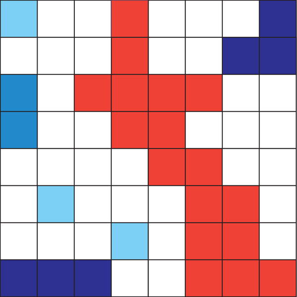
Consider a square lattice as shown in Fig. 1. In the figure, the occupied sites are denoted in color. Percolation theory studies the clusters that are formed by the occupied sites. Of particular interest is systems at the onset of percolation, where a cluster extends from one edge of the system to the opposite edge for the first time (the red cluster in Fig. 1). The percolation model was originally defined by occupying the sites randomly. However, as we will see, images are mapped to a correlated percolation model: if a site is occupied it is more likely for its nearest neighbors to be occupied as well.

Fig. 1.

Percolation in 2d square lattice of size L = 8. The “occupied” sites are shown in color, sites in the same cluster are colored uniformly and different colors denotes clusters of difference sizes. In this example, there are three clusters of size 1 (n₁ = 3/64), one cluster of size 2 (n₂ = 1/64), two clusters of size 3 (n₃ = 2/64), and there is a percolating cluster of size 17 (n₁₇ = 1/64, M(L = 8) = 17) shown in red. See Fig. 7 for the scaling of M(L) and n_s in images.

A cluster is defined as a group of nearest-neighbor squares that are occupied. Percolation theory deals with studying clusters that are formed. In Fig. 1, occupied sites that belong to a cluster are colored uniformly. The size of a cluster s is defined as the number of sites inside that cluster. In the figure, clusters that have the same size are given the same color. There are three clusters of size s = 1, one cluster of size s = 2, etc. The cluster number n_s is defined as the number of clusters with s sites per lattice site, e.g., n₂ = 1/64 in this example. Later in the paper, we will study n_s for images, which take the power-law form n_s ∝ s^−τ.

Fig. 1 also introduces the concept of percolating cluster (the cluster in red), defined as a cluster which extends from one edge of the lattice to its opposite edge. A percolating cluster is also known as an “infinite” cluster, because in the thermodynamic limit (i.e., for an infinite system) its size becomes infinite. Percolation theory was developed to study properties of percolating clusters. Of particular interest are systems at the onset of percolation, at which an infinite cluster appears for the first time. Scale invariance emerges near the percolation transition, which we exploit in our model.

Next we discuss the simplest example of the percolation transition, where sites/pixels are occupied randomly on the square lattice with the occupation probability p. The system can be tuned to be at the onset of percolation by varying p. Images are different from this model, but it will provide intuition about the percolation transition. For the percolation problem, the size of the infinite cluster M(L) normalized by the number of sites in the lattice is the percolation order parameter P = M(L)/L², and is used to describe the degree of percolation order in the system. It is intuitively clear that for small p percolating cluster cannot form since the sites are rarely occupied, therefore P = 0, and the system is disordered. For p = 1 all the sites are occupied and the percolating cluster is the whole lattice: P = 1, and the system is fully ordered. We therefore expect a phase transition from disorder to order for the intermediate values of p. What needs to be verified is that the phase transition is continuous.

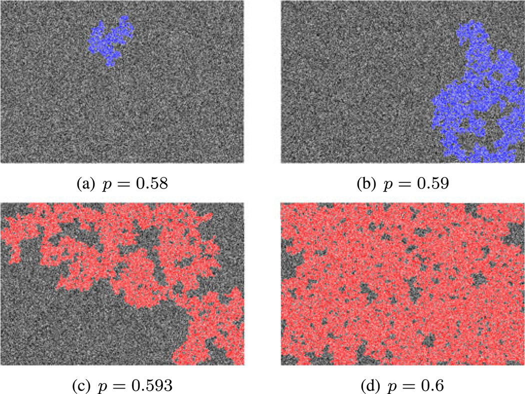
This model despite its simplicity does not have an exact solution at present but the continuous phase transition (known as second-order phase transition in physics) is verified by numerical experiments. The occupation probability, which marks the onset of the percolation transition and the formation of infinite clusters is p_c = 0.59274621 [5]. In the thermodynamic limit, for all p > p_c there is a cluster extending from one side of the system to the other, whereas for all p < p_c no such infinite cluster exists. Percolation order parameter P is zero at p = p_c and rises monotonically for p > p_c. The plot of samples before p < p_c and after p > p_c are given in Fig. 2. In the figure, the largest cluster in the disordered phase p < p_c is singled out in blue. The percolating clusters in the ordered phase p > p_c are singled out in red.

Fig. 2.

Samples from the percolation model before and after the phase transition. The system size is 1,024 × 1,536 pixels, the same as the van Hateren database. The white pixels are empty sites, which are occupied with black pixels at random. The occupation probability is given under each sample. The phase transition on the square lattice happens at the occupation probability p_c = 0.59274621. In (a) and (b) (p < p_c, disordered) the largest cluster is singled out in blue. In (c) and (d) (p > p_c, ordered) the percolating cluster is singled out in red.

Percolation theory provides a natural framework for quantifying scale invariance and the hierarchy of objects sizes in natural images. They key concept is that of clusters. In the next section we map natural images to the percolation model, which becomes the foundation for studying the geometric aspect of the scale invariance in natural images.

3 Binary Representation of Images

How can we map images to the percolation model? A binary representation will provide a natural framework, where the notion of “occupied” and “unoccupied” sites are taken by 0 and 1 pixel values. Our focus in this paper is on gray-scale images, where pixel values are in the range [0, I_max], 0 representing the darkest point, I_max the brightest. Color images can be analyzed the same way in red, green and blue (RGB) channels. An analog value I (assumed to be integer here for simplicity) can be mapped to a binary representation {B₁, B₂, …,B_∧} (B_λ ∈ {0, 1}) by the following decomposition:

$$I=\sum _{\lambda =1}^{\mathrm{\Lambda }}{2}^{\mathrm{\Lambda }-\lambda }{B}_{\lambda },$$ (1)

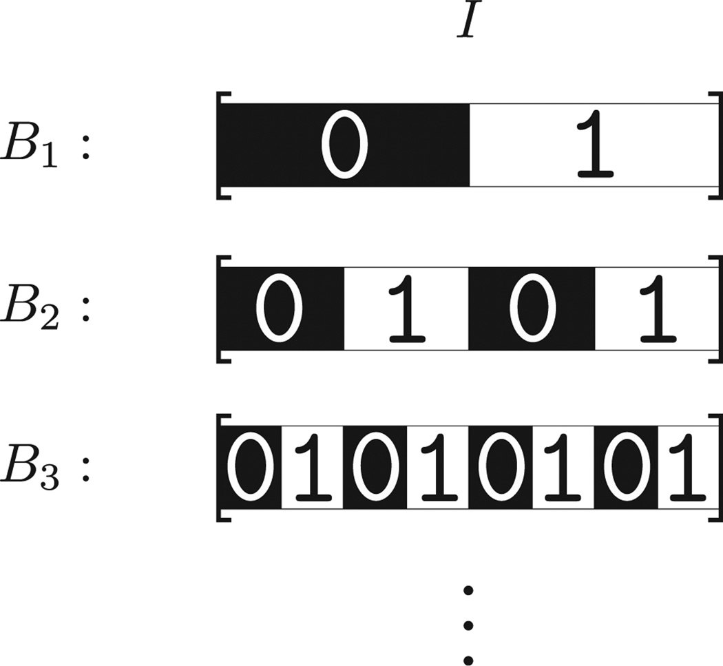
where B_λ is found iteratively by calculating $\lfloor (I-{\sum }_{l=1}^{\lambda -1}{2}^{\mathrm{\Lambda }-l}{B}_l)/2^{\mathrm{\Lambda }-\lambda }\rfloor$ starting from λ = 1, ⌊ ⌋ is the floor function, and ∧ is the the bit-depth of the representation (∧ = ⌊log₂(I_max) + 1⌋), which is ∧ = 15 for the van Hateren database [6]. The visual representation of the map from analog pixel values to its corresponding bits from Eq. (1) is given in Fig. 3.

Fig. 3.

The binary representation for the ∧− bit integer value I in the range [0,2^∧ − 1]. B_λ ∈ {0, 1} is found iteratively by calculating $\lfloor (I-{\sum }_{l=1}^{\lambda -1}{2}^{\mathrm{\Lambda }-l}{B}_l)/2^{\mathrm{\Lambda }-\lambda }\rfloor$ starting from λ = 1, ⌊ ⌋ is the floor function. The map from the analog to binary for the first three bits is shown schematically here, where each bit divide the interval in half iteratively starting from the most significant bit B₁.

In the same manner, the gray-scale image ℐ with non-negative integer values is mapped to a stack of binary images {ℬ₁, ℬ₂, …, ℬ_∧} with pixel values 0,1:

$$ℐ=\sum _{\lambda =1}^{\mathrm{\Lambda }}{2}^{\mathrm{\Lambda }-\lambda }{ℬ}_{\lambda }.$$ (2)

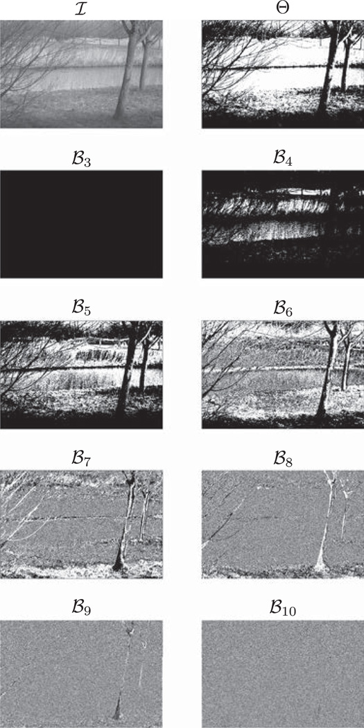
Example of an image ℐ in the van Hateren database, and its corresponding bit planes {ℬ₃, ℬ₄, …, ℬ₁₀} are given in Fig. 4. To emphasize the hierarchy in the representation, we refer to layer λ = 1 as the top layer, and λ = ∧ the bottom one. There is a qualitative change from“order” to “disorder” from the top layer to the bottom layer [7]. We quantify this qualitative change in the next section using the percolation order parameter we defined in the previous section.

Fig. 4.

Example of an image ℐ from the van Hateren database of natural images [6]. Its median thresholded image Θ, and the bit planes {ℬ₃, ℬ₄, …, ℬ₁₀} are shown.

The binary representation obtained from Eq. (2) is exact. However one can also obtain approximate representations by thresholding an image. This was studied in [8] by thresholding images by their median intensity (Fig. 4):

$$ℐ\to \mathrm{\Theta }=\theta (ℐ-\text{median}(ℐ)),$$ (3)

where θ is the step function. There exists a non-linear relation between median-thresholded images and the representation {ℬ₁, ℬ₂, …, ℬ_∧} as follows. The average median intensity for images in the van Hateren database is the value 2¹⁵⁻⁶ < 637 < 2¹⁵⁻⁵. Therefore, on average, activation of a pixel in any of the bit planes above layer 6 (λ ≤ 6) will make the pixel value greater than the median. The median-thresholded images Θ can therefore be obtained by combining ℬ_λ above layer 6 using the logical OR operator [9]:

$$\mathrm{\Theta }=\theta (ℐ-\text{median}(ℐ))\simeq {ℬ}_1\vee {ℬ}_2\vee \cdots \vee {ℬ}_6.$$ (4)

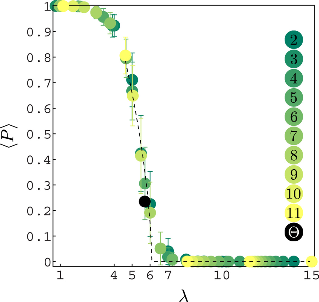
We applied our analysis for layers ℬ_λ to the ensemble Θ. As we will see, the median-thresholded images Θ are close to a percolation transition (Fig. 6), and they lie between layer 5 and 6 in the scaling analysis of clusters (Fig. 7).

Fig. 6.

Plot of the average percolation order parameter < P > for natural images for binary and general base decomposition b = {2, 3, …, 11} (color-coded in the figure) as a function of λ. The λ in base b is transformed to base 2 by the relation ⌊log₂(I_max) + 1⌋− log₂(b^{⌊log_b(I_max)+1⌋−λ}). The standard deviation is indicated by the error bars. The black curve is the best fit near the phase transition P = θ(λ_c − λ) (λ_c− λ)^β/C (where θ is the step function) was obtained for λ_c = 6.1; β = 0.6, C = 1.6. Percolation order parameter was also calculated for the ensemble Θ and is given in black at the position λ = 5.7 obtained from the average median values in the van Hateren database.

Fig. 7.

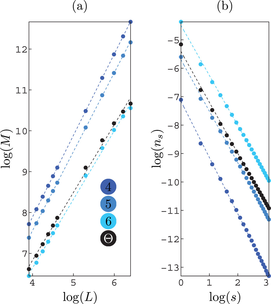
(a) Plot of the size of the percolating clusters M(L) as a function of L, obtained by taking random samples of size L × L from bit planes λ = {4, 5, 6}, and for the ensemble Θ (see Fig. 4). The fractal dimension D: M(L) ∝ L^D obtained from the linear fit in the log-log scale is given in Table 1. (b) Plot of n_s (the number of s-clusters per lattice site) as a function of s. The exponent τ: n_s ∝ s^−τ obtained from the linear fit in the log-log scale is given in Table 1.

4 Percolation Order Parameter and Correlated Percolation Transition

The map from analog images ℐ to the binary representation {ℬ₁, ℬ₂, …, ℬ_∧} is the starting point for defining the percolation model for images. We define pixels with value 1 (white) empty, and pixels with value 0 (black) occupied. A cluster is defined as a group of nearest-neighbor pixels that are occupied as in Figs. 1 and 2. The reason behind the choice 0 ≡ “occupied” and 1 ≡ “empty” is as follows. Only with this choice the top layers, which we consider “ordered” in our model, have the percolation order parameter close to 1. If we had chosen pixels with value 0 as empty the percolation order parameter would have been zero for the top layers, and indistinguishable from the bottom layer regarding percolation. This will become clear shortly.

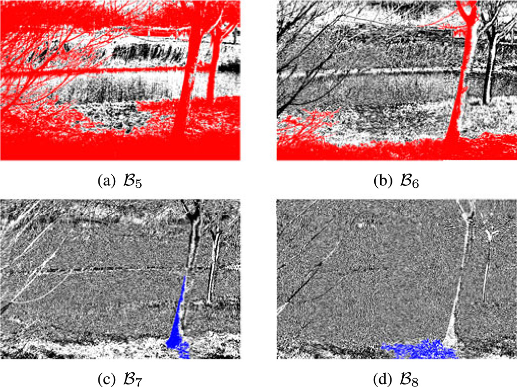
The percolation properties for the top (ordered) and bottom (disordered) layers in the image decomposition {ℬ₁, ℬ₂, …, ℬ_∧} are easily understood. The top layers are mostly 0 (occupied) and the percolation order parameter P ≈ 1 (see Fig. 6). For the bottom layers the pixel values are uniformly distributed and not correlated (white noise). This maps to the classic percolation model on the square lattice with occupation probability p = 0.5 < p_c we discussed earlier (Section 2, Fig. 2). Therefore percolation order parameter P = 0 for the bottom layers. In Fig. 5, we highlight the percolation clusters for bit planes ℬ₅ and ℬ₆ (from Fig. 4) close to the percolation phase transition. In the same figure, bit planes ℬ₇ and ℬ₈ are in the disordered phase and not percolating, but we highlight the largest cluster in blue.

Fig. 5.

This figure singles out the percolating clusters (shown in red) of the bit planes ℬ₅ and ℬ₆. For bit planes ℬ₇ and ℬ₈ which are not percolating the largest cluster is singled out in blue. Notice that in comparison with Fig. 2, the percolating clusters are much more structured, which highlights the fact that this is a correlated percolation phase transition.

We study the percolating properties of all bit planes for all the images in the van Hateren database. The plot of the average of the percolation order parameter < P > vs. λ is given in Fig. 6. Here as in [7] we also considered non-binary systems by forming the decomposition of Eq. (2) in base b > 2. Like the binary case, P was determined by finding percolating clusters of 0 (ignoring nonzero pixel values), λ in base b was then mapped to base 2 by the relation ⌊log₂(I_max) + 1⌋ − log₂(b^{⌊log_b(I_max)+1⌋−λ}), which may not necessarily be an integer. Non-binary decomposition was therefore considered to have some limited continuity (away from integer values) in the “tuning” parameter λ. We fit second-order phase transition curve P = θ(λ_c − λ) (λ_c − λ)^β/C near the phase transition, where the best fit was obtained for λ_c = 6.1, β = 0.6, C = 1.6. We emphasize that the percolation transition here is correlated, since the pixels near layer 6 are correlated [7]. The percolating cluster for layer 6 of Fig. 4 is singled out in red in Fig. 5b. The percolating cluster is highly structured, which highlights the fact that this is a correlated percolation transition.

5 Geometric Characterization of the Scale Invariance in Natural Images

Percolation theory provides the framework to characterize a geometric view of the scale invariance in natural images by studying the scaling properties of the clusters that emerge in the model. Instead of studying the second-order correlation function of pixel intensities, we are concerned with A) How the size the percolating clusters M(L) scale as a function of the system size L, B) How n_s, the number of clusters with size s per lattice site, scales as a function of s. Next we study the scaling properties of these two quantities. Near the percolation transition both these quantities take power law forms with anomalous exponents deviating from mean-field values. See Fig. 1 for a review of the definitions of M(L) and n_s.

5.1 Fractal Dimension

Fractal structures are ubiquitous in nature from coastlines to turbulent flows [4]. It is perhaps not surprising to see signatures of fractals in natural images. In our formulation fractal dimensions appear in the scaling properties of the percolating clusters close to the phase transition. Near the percolation transition the infinite cluster has many holes in it, where some of them could be large. The size of the largest hole is a measure of the correlation length ξ, which becomes “infinite” at the percolation transition. Because of these holes, which appear in all scales, the size the percolating cluster does not scale with an integer Euclidian dimension, instead with a fractal non-integer dimension. The fractal dimension D is the effective dimension for how M grows with the system size L: M ∝ L^D.

The dimension D deviates from the Euclidean dimension near the percolation transition for length scales below the correlation length. Thus for length scales L < ξ, M(L) ~ L^D with D < 2. For length scales L > ξ the Euclidean dimension D = 2 is recovered. The dimension D is obtained by taking L × L samples and finding the linear fit in the log-log scale (Fig. 7, Table 1). The curve deviates from linear for large L (when it is comparable to system size) due to limited sampling, which were not used for obtaining the exponents.

TABLE 1.

Exponents D and τ

	λ = 4	λ = 5	λ = 6	Θ
D	1.99	1.93	1.68	1.66
τ	1.98	1.81	1.76	1.79

5.2 Scale-Invariant Distribution of Cluster Sizes

Another signature of scale invariance at the percolation transition is that the distribution of number of clusters as a function of their size takes a power-law form. The number of clusters of size s (s-clusters) per lattice site is denoted by n_s. Large clusters are less frequent than smaller clusters. Above the critical point, n_s takes the algebraic form n_s ∝ s^−τ, where τ is close to 2 away from the critical point, and becomes anomalous deviating from the mean-field value τ = 2 at the critical point [10]. This scaling is demonstrated in Fig. 7b for layers {4, 5, 6} and the exponents t are given in Table 1.

6 Clusters for Image Segmentation

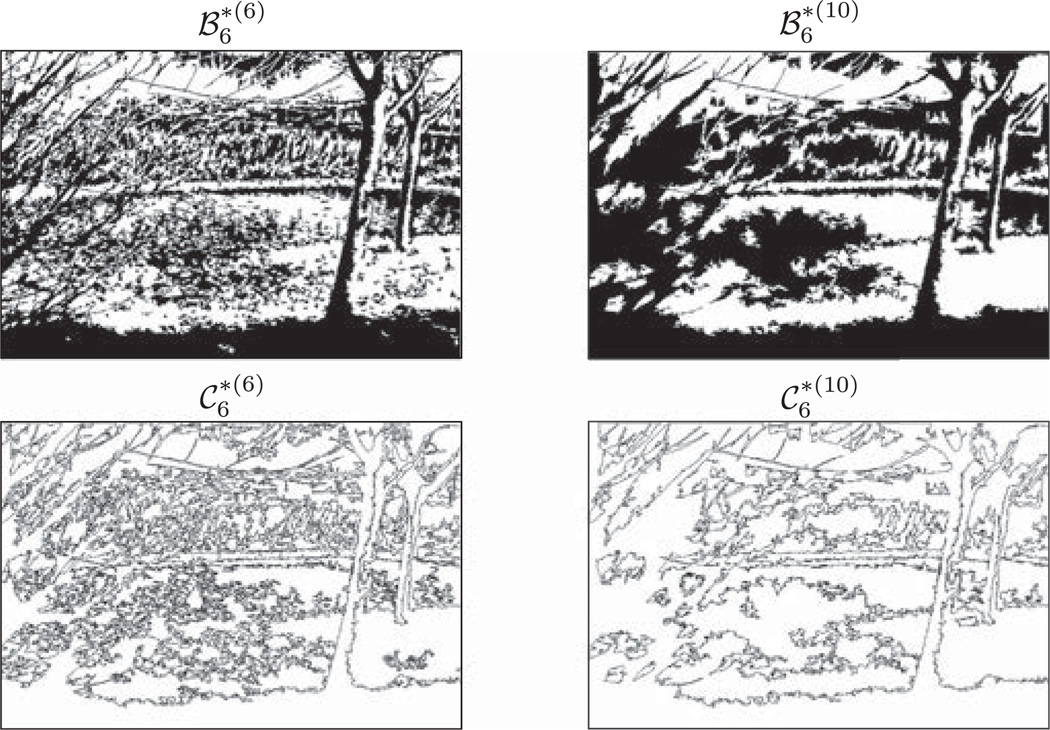
In this section we outline an application of the framework we introduced here in identifying clusters in images for image segmentation and edge detection [11]. For the case of binary (b = 2) decomposition, the clusters of 1 and 0 in each layer ℬ_λ segment the image into regions. By analogy, clusters of 1 form “islands” in the “seas” of 0, and they could correspond to parts of objects in the original image. Furthermore, the islands and seas can be merged if their size is less than a cutoff. We use the notation ${ℬ}_{\lambda }^{*(n)}$ to denote the transformed pixel values after merging clusters of 1 and 0 into their surrounding, i.e., 0 and 1 respectively, if the size of the cluster is less than 2ⁿ (Fig. 8). The boundaries between clusters are then identified as edges denoted by ${𝒞}_{\lambda }^{*(n)}$ (Fig. 8).

Fig. 8.

${ℬ}_6^{*(n)}$ is the layer ℬ₆ of Fig. 4 after dissolving clusters smaller than 2ⁿ into their surroundings. ${𝒞}_6^{*(n)}$ are the corresponding edges between the clusters. They are demonstrated for n = 6 and n = 10.

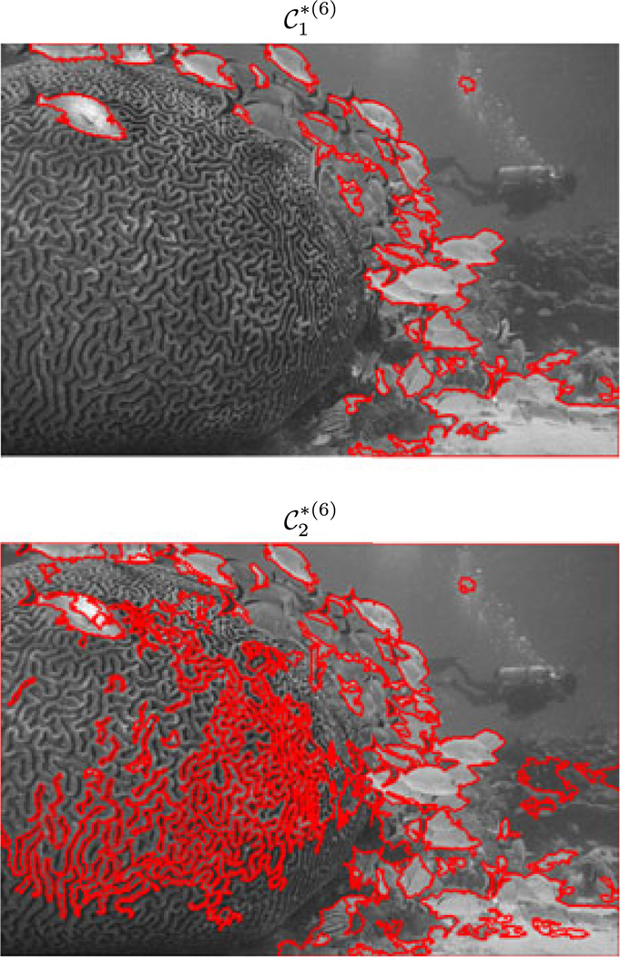
This approach at the current stage is limited as can be seen by looking at an example of the Berkeley segmentation database in Fig. 9. These images are jpeg with the bit-depth of L = 8 (as opposed to 15 in the van Hateren database) [12]. The bit-depth disparity requires a different analysis when it comes to the information content of different bit planes. For example for the jpeg image shown in Fig. 9 the median intensity is 2⁸⁻² < median(ℐ) = 86 < 2⁸⁻¹, the median-thresholded image thus lies between layer 1 and 2 in the binary decomposition. The boundaries between clusters for layer 1 and 2 in this example are highlighted in red in Fig. 9. We emphasize that in this approach different layers give rise to different segments and it is an open question how to integrate different segmentations thus obtained.

Fig. 9.

Example of an image in the Berkeley segmentation database. The top figure highlights in red the boundaries ${𝒞}_1^{*(6)}$ of the clusters in the first layer ℬ₁ after dissolving clusters of size smaller than 2⁶. The bottom figure is the same but for layer two ℬ₂. This figure highlights the limitations of the correspondence between clusters and image segments at the present stage.

In the mainstream approach to image segmentation, one is interested in smooth contours for traces of objects. However for natural images, they will not necessarily be smooth especially for textures and fractal structures in images. A strength of our approach is the capability to segment structures in natural images that do not necessarily have smooth boundaries. We have also introduced a notion of scale in image segmentation for natural images based on introducing a cutoff for cluster sizes. But more work needs to be done for finding meaningful semantics for the clusters and integrating different clusters across different bit planes.

On the conceptual level, the picture we have provided here is appealing because clusters could be large and edges detected this way were not obtained by a local (Gabor-like) filter. The problems with the view of primary visual cortex as a “Gabor filter bank” and its limitations in computer vision applications are discussed by Olshausen and Field [13].

7 Discussion

What would the “ultimate theory” for the scale invariance of natural images look like? The well-established framework in physics for understanding scale invariance is the renormalization group, which explains the scale invariance found in nature in a single framework. The renormalization group is based on removing high spatial/temporal frequency fluctuations in a hierarchical fashion, and finding how interactions change by this process. It is powerful for explaining systems with “fluctuations in structure over a vast range of sizes” [14]. We know that the key signature of natural images is that they have structures over a vast range of sizes, but how can we formulate the renormalization group for images? Answering this question is especially timely for machine learning and the deep learning community in light of the recent observations about connections between deep learning and the renormalization group [15]. The renormalization group’s behavior is especially well-understood for systems near second-order phase transitions and our results for the percolation phase transition in natural images lays the foundation for studying the renormalization group for images.

References

- 1.Simoncelli EP, Olshausen BA. Natural image statistics and neural representation. Annu. Rev. Neurosci. 2001;24(1):1193–1216. doi: 10.1146/annurev.neuro.24.1.1193. [DOI] [PubMed] [Google Scholar]
- 2.Ruderman DL. Origins of scaling in natural images. Vis. Res. 1997;37(23):3385–3398. doi: 10.1016/s0042-6989(97)00008-4. [DOI] [PubMed] [Google Scholar]
- 3.Ruderman DL, Bialek W. Statistics of natural images: Scaling in the woods. Phys. Rev. Lett. 1994 Aug.73:814–817. doi: 10.1103/PhysRevLett.73.814. [DOI] [PubMed] [Google Scholar]
- 4.Mandelbrot BB. The Fractal Geometry of Nature. New York, NY, USA: Macmillan; 1983. [Google Scholar]
- 5.Newman M, Ziff R. Efficient Monte Carlo algorithm and high-precision results for percolation. Phys. Rev. Lett. 2000;85(19):4104. doi: 10.1103/PhysRevLett.85.4104. [DOI] [PubMed] [Google Scholar]
- 6.van Hateren JH, van der Schaaf A. Independent component filters of natural images compared with simple cells in primary visual cortex. Proc. Roy. Soc. London. Series B: Biol. Sci. 1998;265(1394):359–366. doi: 10.1098/rspb.1998.0303. [DOI] [PMC free article] [PubMed] [Google Scholar]
- 7.Saremi S, Sejnowski TJ. Hierarchical model of natural images and the origin of scale invariance. Proc. Nat. Acad. Sci. USA. 2013 Feb.110(8):3071–3076. doi: 10.1073/pnas.1222618110. [DOI] [PMC free article] [PubMed] [Google Scholar]
- 8.Stephens GJ, Mora T, Tkčik G, Bialek W. Statistical thermodynamics of natural images. Phys. Rev. Lett. 2013 Jan.110:018701. doi: 10.1103/PhysRevLett.110.018701. [DOI] [PubMed] [Google Scholar]
- 9.Saremi S, Sejnowski TJ. On criticality in high-dimensional data. Neural Comput. 2014;26(7):1329–1339. doi: 10.1162/NECO_a_00607. [DOI] [PMC free article] [PubMed] [Google Scholar]
- 10.Stauffer D, Aharony A. Introduction to Percolation Theory. Boca Raton, FL, USA: CRC Press; 1994. [Google Scholar]
- 11.Shi J, Malik J. Normalized cuts and image segmentation. IEEE Trans. Pattern Anal. Mach. Intell. 2000 Aug.22(8):888–905. [Google Scholar]
- 12.Martin D, Fowlkes C, Tal D, Malik J. A database of human segmented natural images and its application to evaluating segmentation algorithms and measuring ecological statistics. Proc. 8th Int. Conf. Comput. Vis. 2001 Jul.2:416–423. [Google Scholar]
- 13.Olshausen BA, Field DJ. How close are we to understanding V1? Neural Comput. 2005;17(8):1665–1699. doi: 10.1162/0899766054026639. [DOI] [PubMed] [Google Scholar]
- 14.Wilson K. Problems in physics with many scales of length. Sci. Am. 1979;241:158–179. [Google Scholar]
- 15.Mehta P, Schwab DJ. An exact mapping between the variational renormalization group and deep learning. arXiv:1410.3831. 2014 [Google Scholar]