Abstract
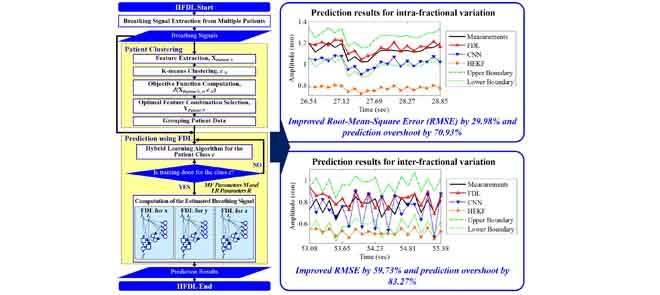
Tumor movements should be accurately predicted to improve delivery accuracy and reduce unnecessary radiation exposure to healthy tissue during radiotherapy. The tumor movements pertaining to respiration are divided into intra-fractional variation occurring in a single treatment session and inter-fractional variation arising between different sessions. Most studies of patients’ respiration movements deal with intra-fractional variation. Previous studies on inter-fractional variation are hardly mathematized and cannot predict movements well due to inconstant variation. Moreover, the computation time of the prediction should be reduced. To overcome these limitations, we propose a new predictor for intra- and inter-fractional data variation, called intra- and inter-fraction fuzzy deep learning (IIFDL), where FDL, equipped with breathing clustering, predicts the movement accurately and decreases the computation time. Through the experimental results, we validated that the IIFDL improved root-mean-square error (RMSE) by 29.98% and prediction overshoot by 70.93%, compared with existing methods. The results also showed that the IIFDL enhanced the average RMSE and overshoot by 59.73% and 83.27%, respectively. In addition, the average computation time of IIFDL was 1.54 ms for both intra- and inter-fractional variation, which was much smaller than the existing methods. Therefore, the proposed IIFDL might achieve real-time estimation as well as better tracking techniques in radiotherapy.
Keywords: Fuzzy deep learning, intra-fractional variation, inter-fractional variation, breathing prediction, tumor tracking
This paper presents the validation in human subjects of a new approach to tracking lung-cancer tumor motion, which poses a significant challenge for precise dose delivery in lung cancer radiotherapy. Intra- and Inter-fraction Fuzzy Deep Learning (IIFDL) is a new predictor for intra- and inter-fractional data variation, where FDL, equipped with breathing clustering, predicts the movement accurately and decreases the computation time. Experiment results showed that IIFDL improved Root-Mean-Square Error (RMSE) and prediction overshoot, compared with existing methods. In addition, the average computation time of IIFDL was 1.54ms for both intra- and inter-fractional variation, which was much smaller than existing methods. The proposed IIFDL might achieve real-time estimation as well as better tracking techniques in radiotherapy.
I. Introduction
Lung cancer is the most deadly cancer disease with an estimated 27% of all cancer deaths [1], [2]. A large part of patients with lung cancer undergoes radiotherapy. Tracking tumor motion poses a significant challenge for precise dose delivery in lung cancer radiotherapy, due to respiratory motion of up to 3.5 cm for primary lung tumors [3]–[9]. If the patient’s breathing motion is not correctly predicted, tumor miss might occur, or sensitive normal tissue might be undesirably exposed resulting in unwanted treatment toxicity [10]–[12]. Advanced technologies of radiotherapy, intensity modulated radiotherapy and image guided radiotherapy, may offer the potential of precise radiation dose delivery for moving objects. However, they still need an additional function to predict the precise position of the tumor against subtle variations in real-time [5], [13]–[16].
Radiation dose is typically delivered in 3 to 5 fractions over 5 to 12 days for early stage lung cancer using stereotactic radiotherapy or 30 to 33 fractions over 6 to 7 weeks for more advanced disease with each fraction lasting between 10 and 45 minutes. The patient’s breathing motions during these fractions are broadly divided into two categories [17]–[19]: 1) intra-fractional and 2) inter-fractional variations. Intra-fraction motion indicates changes where the patient is undergoing the radiation therapy, which turns up on a time scale of seconds to minutes [17], [18], [20]–[23]. Each individual shows different breathing patterns. On the other hand, inter-fraction motion is the variation observed between different treatment sessions. It covers breathing motion as well as external factors such as baseline shifts. Inter-fractional variation is typically shown in a time scale of minutes to hours or a day-to-day level [17], [18], [21]–[24].
Inter-fractional motion is distinguishable from intra-fractional movement because the inter-fractional variation covers even baseline shifts and weight gain or loss [21], [22]. However, most studies of breathing prediction so far have focused on respiratory motions within the single treatment session, i.e., intra-fractional variation [6]–[8], [13], [20]–[35]. Recently, several studies [10]–[12] have pointed out the difference between intra-fractional and inter-fractional movements and have discussed the importance of inter-fractional variation in radiation treatment or related imaging techniques. Table 1 summarizes the comparison between intra- and inter-fractional movements.
TABLE 1. Comparison Between Intra- and Inter-Fractional Variations.
| Variation Type | Intra-fraction | Inter-fraction |
|---|---|---|
| Time of Occurrence | During a single fraction [17], [19]–[23] | Between different fractions [19], [20], [22], [23] |
| Time Scale | Seconds to minutes [18] | Hours or day-to-day level [17], [18], [21] |
| Motion Coverage | Internal organ motion, breathing, swallowing [21], [22] | Position changes of patients, patient weight gain/loss, internal organ motion, breathing, swallowing [21], [22] |
Prediction methods for intra-fractional variation have been addressed in many studies [6], [9]–[11], [13], [15], [20], [26]–[38] as illustrated in Table 2. However, inter-fractional variation has not been actively studied as much as intra-fractional motion yet despite its necessity in radiotherapy [9]–[11], [13], [20], [25]–[35]. Intra- and inter-fractional variation of breathing motion can raise many challenges for respiratory prediction [6]–[8], [20], [22], [23], [25]–[35]: Firstly, prediction accuracy should be high. Secondly, computing time should be short enough for real-time prediction. Thirdly, the novel method should be able to handle any unpredictable breathing variation.
TABLE 2. Previous Prediction Methods for Intra- and Inter-Fractional Variations.
| Method | Description | Drawback | Variation |
|---|---|---|---|
| Margin-based [25] | • Compensated locational changes of the tumor in a primitive way, adding extra margins | • High possibility of over/under-dose since the margin is determined by motion range of the tumor without knowing its variation | Intra-/inter-fraction |
| Linear Predictive model (LP) [15], [26] | • Estimated the future state based on functions comprised of linear combination of input data, proper coefficients, and constants | • Inferior prediction accuracy for breathing signals with a long latency • Poor performance improvement by its exclusive usage • Assumption that the nonlinear respiratory movement is linear |
Intra-/inter-fraction |
| Adaptive Filter (AF) [6], [9], [15], [27]–[31], [36] | • Combined modified LPs and additional filters that adjust coefficients of LPs | • No guarantee of its superb performance in most cases because it highly depends on adaptation intervals | Intra-fraction |
| Kalman Filter (KF) [26], [29], [32], [33] | • Efficient recurrent filter which has been utilized in various forms: Kalman constant velocity, Kalman constant acceleration, an interacting multiple model, and Hybrid implementation based on the Extended KF (HEKF) | • Only adaptable to linear or nearly linear estimation • High computation complexity of KF-based models combined with other prediction tools |
Intra-fraction |
| Artificial Neural Network (NN)-based [10], [11], [13], [15], [20], [26], [27], [30], [32]–[35], [37], [38] | • Showed outstanding accuracy for irregular patterns and abrupt changes, • Extended approaches: back propagation NN, feed-forward NN, recursive NN, wavelet NN, Customized prediction with multiple patient interactions using NN (CNN), and HEKF |
• Long calculation time for prediction parameters and results | Intra-fraction |
| Cubic model [23] | • Estimated respiratory variance by using a third-order polynomial equation | • Same drawback of low accuracy as LP because the cubic model is also one of the mathematic approaches like LP | Inter-fraction |
| Stochastic Fluence Map Optimization (FMO) model [22] | • Extended deterministic FMO model, which assumes that a patient is static • Solved observed problems by employing convex penalty functions and numerous scenarios to characterize inter-fractional uncertainties |
• Unpredictable method for other disregarded scenarios | Inter-fraction |
In this paper, we propose a new prediction approach for intra- and inter-fraction variations, called Intra- and Inter-fractional variation prediction using Fuzzy Deep Learning (IIFDL). The proposed IIFDL clusters the respiratory movements based on breathing similarities and estimates patients’ breathing motion using the proposed Fuzzy Deep Learning (FDL). To reduce the computation time, patients are grouped depending on their breathing patterns. Then, breathing signals belonging to the same group are trained together. Future intra- and inter-fractional motion is estimated by the trained IIFDLs.
The contribution of this paper is threefold. First, this is the first analytical study for modeling multiple patients’ breathing data based on both intra- and inter-fractional variations. Secondly, the proposed method has a clinical impact for enhanced adjustment of margin size because it achieves high prediction accuracy for respiratory motion, even for inter-fractional variation. Thirdly, this study shows the clinical possibility of real-time prediction by largely shortening computing time. Furthermore, the training process can be shortened, by training breathing signals with similar patterns together in the proposed IIFDL.
II. Fuzzy Deep Learning
The proposed FDL is a combination of fuzzy logic and a NN with more than two hidden layers, i.e. deep learning network. Due to the NN architecture of FDL, it has a self-learning feature, setting network parameters by training itself according to input and desired output values. FDL also has a fuzzy logic feature of reasoning capability for uncertainty. In FDL, a few fuzzy parameters, i.e. prediction parameters of FDL, determine weight values between nodes in the network, and weight values are considered as the prediction parameters in other methods. Consequently, the number of prediction parameters is much less than that of other mutated NN methods and parametric nonlinear models. This reduces the computation time substantially and makes suitable for to real-time and nonlinear estimation.
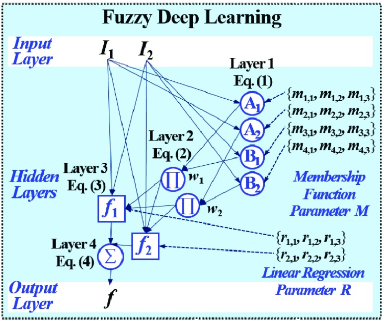
Fig. 1 exemplifies a simple architecture of FDL, including Layer 1 through Layer 4 in the hidden layers. The functions of four hidden layers can be summarized as follows: Layer 1 provides membership functions which are determined by a Membership Function (MF) parameter set  {
{ ,
,  ,
,  }, Layer 2 applies a T-norm operation, Layer 3 computes linear regression functions by normalized weights and a Linear Regression (LR) parameter set
  {
{ ,
,  ,
,  }, and Layer 4 finally yields an output of FDL
  by summing outcomes according to all fuzzy if-then rules.
FIGURE 1.
FDL architecture including Layer 1 through Layer 4 in the hidden layers: Layer 1 provides membership functions, Layer 2 applies a T-norm operation, Layer 3 computes linear regression functions, and Layer 4 finally yields an output of FDL according to all fuzzy if-then rules.
For the training algorithm of FDL, we use the hybrid learning algorithm [36] which is a combination of a gradient descent back-propagation algorithm and a least squares estimate algorithm. The MF parameter and the LR parameter are identified by this training algorithm [36].
In Fig. 1, the number of fuzzy if-then rules is equivalent to that of nodes in Layer 2 and 3, which are given as follows:
-
Rule1:
If
 is
is  and
and  is
is  , then
  ,
, -
Rule2:
If
 is
is  and
and  is
is  , then
where  and
and  are inputs of FDL, and
  and
and  are fuzzy sets, which are linguistic labels.
The output  in Layer 1 is described as follows:
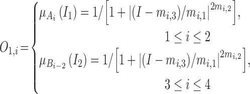 |
where  and
and  are MFs of inputs for each fuzzy set of
  and
and  . Also,
  ,
,  , and
, and  are the MF parameters chosen by the training algorithm.
The functions of Layer 2 multiply all the values coming from Layer 1, as follows:
 |
where multiplication acts as the T-norm operator in the fuzzy system, and the output indicates the firing strength for the rule.
In Layer 3, the linear regression function is applied to a ratio of the  th rule’s firing strength to the summation of all rules’ firing strengths, and its result can be calculated by
 |
where  ,
,  , and
, and  are the LR parameters, derived from the training algorithm.
The output of Layer 4 is aggregate of (3) as follows:
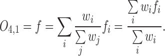 |
The output of FDL is computed by its weights and regression functions as (4).
III. Intra- and Inter-Fractional Variation Prediction Using Fuzzy Deep Learning
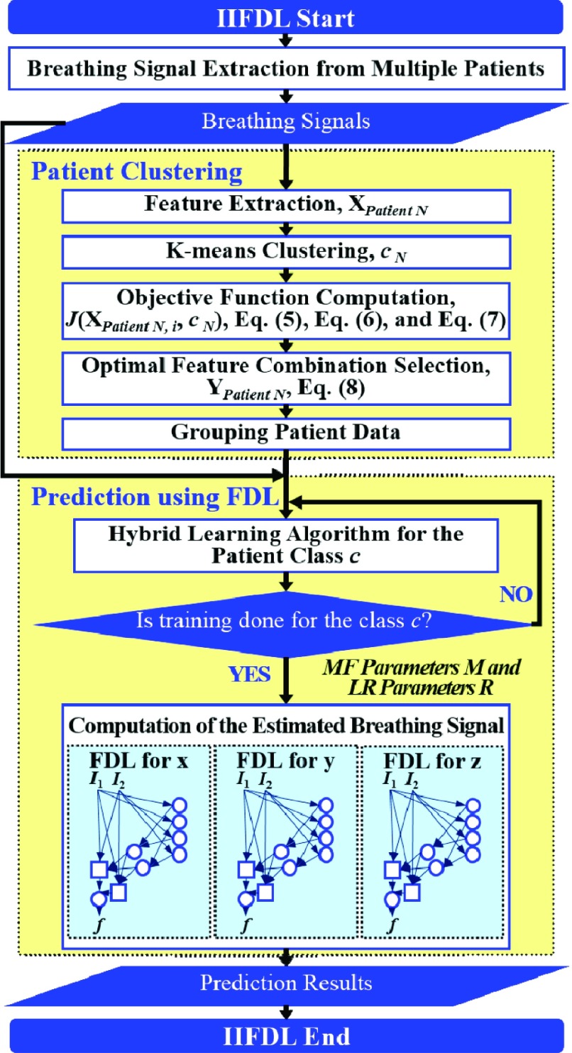
The proposed IIFDL is designed to reduce the computational complexity of prediction for multipatients’ breathing motion, which occurs during the single treatment session and between treatment sessions. To achieve this, the proposed IIFDL clusters multiple patients based on their breathing feature similarities and trains their respiratory signals for each group. We illustrate the process of IIFDL in Fig. 2. Before the detailed explanation of IIFDL, a summary of its whole process is given as follows:
-
1)
Patient Clustering: Patients’ breathing feature metrics are computed from the respiratory signals, and then patients are clustered according to their breathing feature similarities.
-
2)
Prediction Using FDL: For each patient group, the training procedure of the hybrid learning algorithm is conducted, and then breathing signals with intra-fractional variation or inter-fractional variation are predicted using FDL.
FIGURE 2.
IIFDL procedure including two main parts: patient clustering and prediction using FDL.
We describe the specific clustering procedure in Subsection  first, and we explain FDL for intra- and inter-fractional variation prediction in Subsection
  .
.
A. Patient Clustering Based on Breathing Features
From patients’ respiratory signals, we extract breathing features as clustering criteria: Autocorrelation Maximum (AMV), ACCeleration variance (ACC), VELocity variance (VEL), BReathing Frequency (BRF), maximum Fourier Transform Power (FTP), Principal Component Analysis coefficient (PCA), STandard Deviation of time series data (STD), and Maximum Likelihood Estimates (MLE). Table 3 summarizes features extracted from the signals and their formula. In Table 3, AMV is an indicator of the breathing stability, and ACC, VEL, and STD are directly relevant to respiratory signals [16], [33], [37]. In addition, we use the typical vector-oriented features PCA and MLEas well as other breathing characteristics such as BRF and FTP [16], [33], [38]. There are two improvements in the proposed patient clustering: the removal of unnecessary breathing feature metrics, and the use of clustering criteria with vector forms.
TABLE 3. Features Extracted From the Signals.
| P | Formula | Used form in IIFDL | Used form in [33] |
|---|---|---|---|
| AMV |
 ( ( : period of observations) : period of observations) |
 ( ( vector) vector) |
 (Scalar) (Scalar) |
| ACC |
 ( ( : observed respiratory data) : observed respiratory data) |
 ( ( vector) vector) |
 (Scalar) (Scalar) |
| VEL |  |
 ( ( vector) vector) |
 (Scalar) (Scalar) |
| BRF |
 (n( (n( ): number of breathing cycles, and ): number of breathing cycles, and  th breathing cycle range) th breathing cycle range) |
 ( ( vector) vector) |
 |
| FTP |
 ( ( : number of breathing signal samples, 1≤ k ≤ N) : number of breathing signal samples, 1≤ k ≤ N) |
 ( ( vector) vector) |
 (Scalar) (Scalar) |
| PCA | PrinComp (PrinComp( (PrinComp( : PCA function, Z: data matrix ( : PCA function, Z: data matrix ( , ,  )) )) |
 ( ( vector) vector) |
 (Scalar) (Scalar) |
| STD |
 ( ( : ith breathing signal sample, and : ith breathing signal sample, and  ’: average of breathing signal samples) ’: average of breathing signal samples) |
 ( ( vector) vector) |
 (Scalar) (Scalar) |
| MLE |
 ( ( : normal distribution) : normal distribution) |
 ( ( vector) vector) |
 (Scalar) (Scalar) |
Firstly, previous studies in [16], [27], [33], [35], [37], and [38] chose two additional feature metrics, i.e. autocorrelation delay time (ADT) and multiple linear regression coefficients (MLR), in addition to those eight in Table 3 for respiratory pattern analysis. However, ADT depends on the length of breathing signal samples, rather than the individual respiration characteristics. The use of MLR assumes that breathing signals are linear, fixed values, and homoscedasticity. This does not correspond to the respiratory signals [33]. For these reasons, we do not select ADT and MLR as breathing features for patient clustering.
Secondly, the existing study [33] clustered patients based on the magnitude values of their respiratory feature vectors. However, the proposed method uses breathing feature vectors for patient clustering, not their magnitude values. For example, the proposed IIFDL analyzes the similarities among patients’ PCA by comparing each component of  vector
  , but the previous method in [33] calculates the similarities based on the scalar value of
  . Accordingly, the previous method clusters patients as the same group when the breathing signals have the approximate magnitude of the breathing feature vector, even though they do not show the similar breathing features. Thus, the proposed IIFDL compares each component of breathing feature vectors, so that it can provide better clustering of breathing signals than existing methods.
As shown in Fig. 2, respiratory signals are randomly selected from multiple patients and used for the breathing feature extraction. Let us define  {
{ ,
,  ,
,  ,
,  ,
,  ,
,  ,
,  ,
,  } as a feature selection metrics set, X as an arbitrary feature combination vector based on P, and Y as an optimal feature combination vector. The total number of possible Xs in the given data is 247 (
 ,
,  ). Among these Xs, Y is selected using a criterion function
  , which is determined by within-class scatter
  and between-class scatter
  values. The within-class scatter
  is defined as follows [16]:
 |
where  is the number of classes less than the total number of patients
  ,
,  and
and  indicate the
  th class and its mean, and
  is the number of patients of Class
  .
.
The between-class scatter  is defined as:
 |
where  is the mean of all feature combination vectors.
With  and
and  , the criterion function
  is given as follows:
 |
This implies that the larger  allows, with low in-class and high inter-class dispersion, the more obvious distinction between classes. After criterion function values are calculated for all Xs and all possible numbers of clusters
  , Y can be decided with the following condition:
 |
After choosing Y by (8), the final number of clusters  is set, and patients are clustered as
  classes depending on selected principal features of Y.
B. Prediction Using FDL
After multiple patients are clustered, we can train patients’ data for each group. For intra-fractional variation, FDL trains parameters based on input data in a single session and predicts future intra-fractional variation. For inter-fractional variation, FDL predicts breathing motion by training the FDL network for multiple datasets of previous sessions. Here, datasets of inter-fractional variation already include the patient’s intra-fractional variation, as described in Section I. Training datasets consist of the initial data and the target data. We train the datasets with the hybrid learning algorithm [36]. During the training procedure, two prediction parameter sets of FDL, i.e., MF parameter set  and LR parameter set R, are obtained and applied to the proposed FDL.
For estimating intra- and inter-fractional variation from the CyberKnife data, FDL has a similar structure to Fig. 1, but the number of nodes is variable. Here, the input datasets consist of three-Dimensional (3D) coordinates for each channel. Thus, we designed the proposed prediction method to have three FDLs for each  ,
,  , and
, and  coordinate, so that we can obtain all 3D coordinates of the estimated breathing signal. Each FDL has three inputs corresponding to three different channels. The total number of nodes in Layer 2 and 3 is 27, based on the number of fuzzy if-then rules, which are given as follows:
-
Rule1:
If
 is
is  and
and  is
is  and
and  is
is  , then
  ,
, -
Rule27:
If
 is
is  and
and  is
is  and
and  is
is  , then
where  ,
,  , and
, and  correspond to inputs from three channels of CyberKnife machine, and
  ,
,  , and
, and  are fuzzy sets.
The output  in Layer 1 is computed as follows:
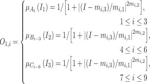 |
where  ,
,  , and
, and  are three kinds of the membership functions, which are calculated using the MF parameter set
  {
{ ,
,  ,
,  }.
}.
In Layer 2 and 3, outputs  and
and  are defined as the following (10) and (11), respectively:
 |
where  ,
,  ,
,  , and
, and  are the LR parameter set
  .
.
The output of Layer 4 is as follows:
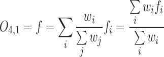 |
The equation (12) produces a single coordinate of the predicted respiratory signal, i.e.,  ,
,  , or
, or  estimation. As mentioned above, the proposed IIFDL uses three FDLs for
  ,
,  , and
, and  coordinates, so that we can derive estimated 3D coordinates of breathing signals from those FDLs.
IV. Experimental Results
We describe the experimental data for intra- and inter-fraction motion, in Subsection  . The experimental result of patient clustering based on breathing features are presented in Subsection
  , and we evaluate the prediction performance of the proposed IIFDL in Subsection
  .
.
A. Intra-and Inter-Fraction Motion Data
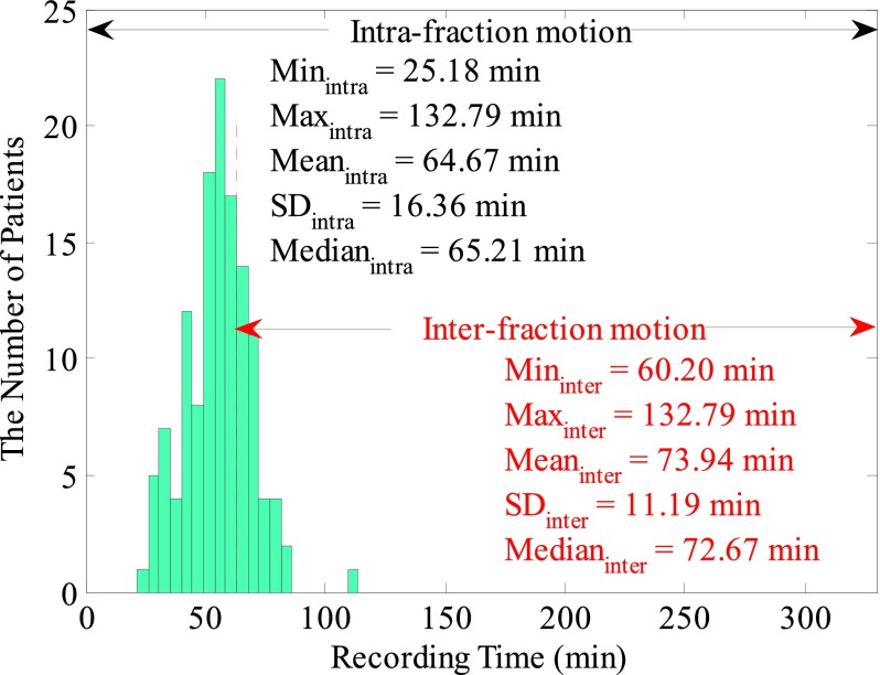
Breathing data of 130 patients were collected in Georgetown University medical center using the CyberKnife Synchrony (Accuray Inc. Sunnyvale, CA) treatment facility. The collected data contained no personally identifiable information, and the research study was approved by the Georgetown University IRB. During data acquisition, three sensors were attached around a target position on the patient’s body. Individual patient’s database contains datasets recorded through three channels by LED sensors and cameras. Fig. 3 illustrates patient distribution for breathing databases according to a record time.
FIGURE 3.
Patient distribution of CyberKnife data. Each database contains a record time, 3D coordinates, and rotation data of three channels. The intra-fractional variation dataset had 130 databases, and the inter-fractional variation dataset consisted of 32 databases with at least 1-hour time difference in-between.
Sampling frequencies for patients’ variation data were 5.20, 8.67, and 26Hz, corresponding to the measurement intervals, 192.30, 115.38, and 38.46ms. The recording time was distributed from 25.13 to 132.52min. Each database contains calibrated datasets of a record time, 3D coordinates, and rotational data of three channels. During the training procedure, we randomly extracted 1000 samples for each patient. The obtained samples regarding the measurement intervals were about 0.63min for 38.46ms, 1.92min for 115.38ms, and 3.2min for 192.30ms.
Table 4 shows experimental data of intra- and inter-fractional variation. In the intra-fractional variation dataset, all of 130 databases were used, and training and test data were randomly selected within 1-hour time range. In the inter-fractional variation dataset, however, we selected 32 databases. Training and test data were selected with at least 1-hour time difference in-between them for the inter-fractional variation dataset. This time scale is not on the day-to-day level as the standard definition of the inter-fractional variation, but it meets the inter-fractional time scale condition of [18]. Actual inter-fractional motion data might be larger than data we chose because changes occurred in fractions on different days such as weight gain or loss were not contained in experimental data.
TABLE 4. Experimental Data.
| Data Type | Intra-fractional Variation | Inter-fractional Variation |
|---|---|---|
| Patient # | 130 | 32 |
| Measurement Intervals (ms) | 38.46, 115.38, and 192.30 | |
| Inputs | Estimated tumor location | |
| Outputs | Next tumor position in the current fraction | |
| Training Data | Previous tumor location data in the current fraction | tumor location data in the previous fractions |
| Test Data | Current tumor location data in the current fraction | current tumor location data in the current fraction |
B. Patient Clustering Based on Breathing Features
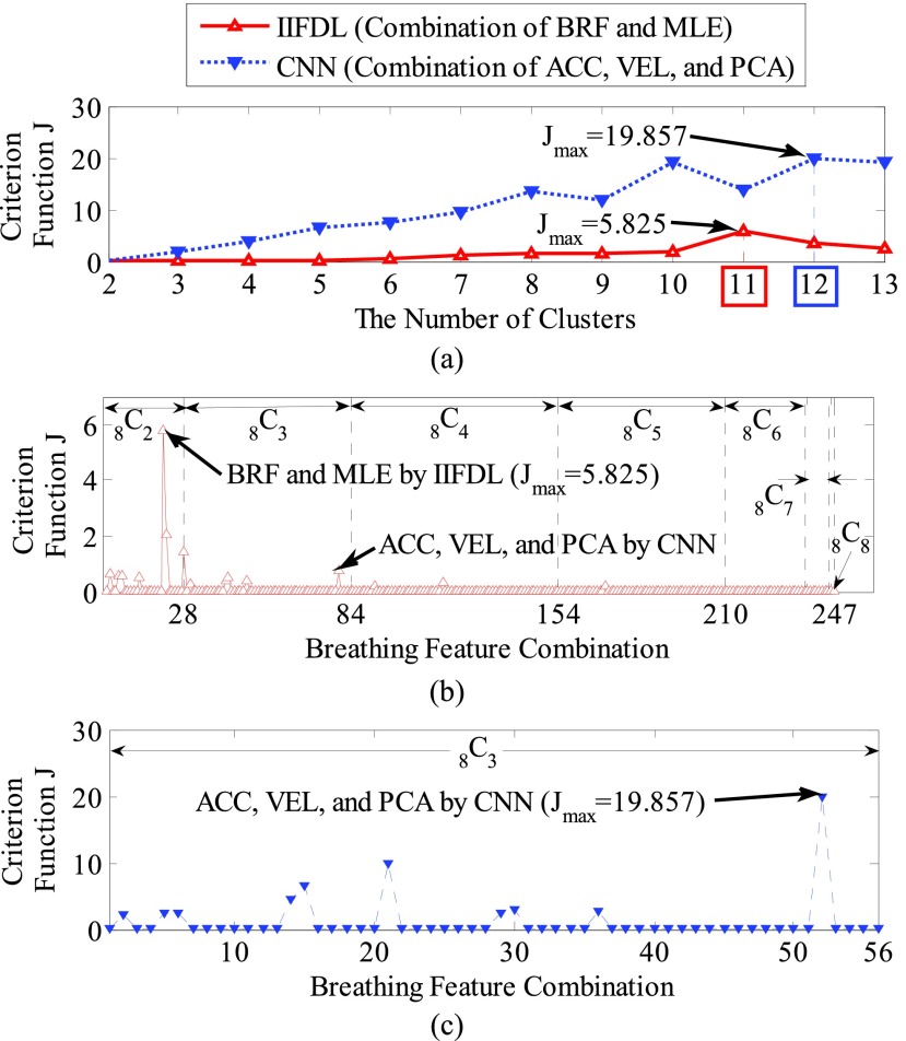
We present the patient clustering results with the calculated criterion function values  . Fig. 4(a) shows criterion function values
  regarding the number of clusters, where we represented the proposed IIFDL as a red line with a ‘
 ’ maker, and the alternate CNN [33] as a blue dotted line with a ‘
 ’ marker. Fig. 4(b) and 4(c) show criterion function values
  of IIFDL and CNN with regard to the possible breathing feature combination.
FIGURE 4.
Criterion function values  of the proposed IIFDL and CNN: (a)
  of IIFDL and CNN according to the number of clusters, (b)
  of IIFDL according to the breathing feature combination, and (c)
  of CNN according to the breathing feature combination. In IIFDL, the number of cluster
  was 11 and the optimal breathing feature combination Y was chosen as BRF and MLE by (8). In CNN,
  was 12 and its Y was a combination of ACC, VEL, and PCA.
The proposed IIFDL selected the number of cluster  as 11 with the maximum
  of 5.825 as shown in Fig. 4(a). The optimal breathing feature combination Y was chosen with BRFand MLE by (8) as shown in Fig. 4(b). The alternate CNN [33] selected the number of cluster
  as 12, and its Y was chosen with ACC, VEL, and PCA as shown in Fig. 4(a) and 4(c). The reason of their different clustering results is that IIFDL uses respiratory feature vectors, whereas CNN uses the magnitude values of respiratory feature vectors. Considered all possible 247 combinations from 8 features (
 ,
,  ), the combination chosen by CNN had a local maximum value of
  , as shown in Fig. 4(b). Thus, the combination of ACC, VEL, and PCA cannot be Ythat has the maximum
  .
.
Therefore, CyberKnife patient databases were grouped into 11 classes using the proposed IIFDL, and the clustering results for intra- and inter-fractional variation data are presented in Table 5.
TABLE 5. Patient Database Clustering.
| Class Number | 1 | 2 | 3 | 4 | 5 | 6 | 7 | 8 | 9 | 10 | 11 | Total | |
|---|---|---|---|---|---|---|---|---|---|---|---|---|---|
| # of Data-bases | Intra-fractional Variation | 1 | 8 | 35 | 2 | 27 | 26 | 1 | 9 | 2 | 1 | 18 | 130 |
| Inter-fractional Variation | 1 | 1 | 10 | 1 | 5 | 6 | N/A | 2 | N/A | 1 | 5 | 32 | |
In Table 5, 130 databases of the intra-fractional variation and 32 databases of the inter-fractional variation were grouped into 11 and 9 classes, respectively. Each class showed the similar breathing features regardless of the variation type. In the intra-fractional variation, some classes (e.g. Class 1, 4, 7, 9, and 10) have only one or two patients. They are most likely considered as the irregular respiratory signals, due to their less feature similarities with other patients’ breathing signals. Class 2 and 8 for the inter-fractional variation also have highly few patients, but we do not consider these classes as the irregular breathing signals. It is difficult to judge the scarcity of Class 2 and 8 based on the few number of intra-fractional variation databases, also these two classes were already considered as regular breathing groups for the intra-fractional variation.
C. Prediction Using FDL
In this subsection, we compare the prediction performance of the proposed IIFDL with existing methods. Especially, previous methods for the inter-fractional movement are mathematical models depending on predefined scenarios of patients’ variation, without the self-learning feature. The prediction performance of these methods is susceptible to how many potential scenarios were considered. In other words, there is a practical limitation to get decent performance results in the experiment with those mathematical models. Accordingly, we chose the existing methods for intra-fractional prediction, CNN and HEKF, as the comparison targets, and we applied the selected methods to the case of the inter-fractional variation. The predictors used in CNN and HEKF are NN and a combination of NN and KF, respectively, as mentioned in Section I. Thus, these methods have the self-learning feature. Furthermore, CNN is the prediction approach designed for multiple patients’ motion like the proposed IIFDL.
We evaluate the prediction performance of IIFDL using by the following three criteria: Root-Mean-Square Error (RMSE), overshoot, and prediction time.
1). Root-Mean-Square Error
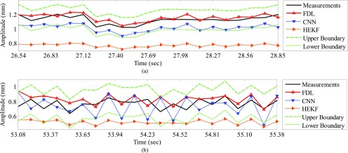
We compared IIFDL with CNN and HEKF regarding prediction results and RMSE. Fig. 5 shows prediction results of two databases by IIFDL, CNN, and HEKF, with 115.38ms interval as a median of [38.46, 192.30ms]. These prediction results were randomly chosen in the given databases. Fig. 5 (a) and 5 (b) present the prediction results of the intra-and inter-fractional variation datasets. Here, a horizontal axis is the time index extracted from CyberKnife data. A black line is a measurement, a red line with a ‘ ’ marker illustrates predicted values by the proposed IIFDL, a blue dotted line with a ‘
 ’ marker is the estimated results of CNN, and an orange dotted line with a ‘
 ’ marker represents the estimation results of HEKF. Also, two green dotted lines are upper and lower boundaries of target data, respectively. These two boundaries were decided based on 95% prediction interval.
FIGURE 5.
Prediction results for (a) intra- and (b) inter-fractional variation by IIFDL, CNN, and HEKF: (a) DB47 and (b) DB121 with 115.38ms interval. The estimated values of the proposed IIFDL were closer to the target values, i.e. measurements, than those of CNN and HEKF.
As shown in Fig. 5, the estimated points of the proposed method IIFDL were closer to the target values than those of CNN and HEKF. In Fig. 5, many points of CNN were distributed near or out of the boundaries, and most of the points of HEKF were out of the range between upper and lower boundaries. However, the predicted values of IIFDL were within the boundaries in most cases. The RMSE comparison of the intra-fractional variation of each patients’ class showed that the proposed IIFDL, CNN, and HEKF had the similar RMSE values overall, and IIFDL outperformed CNN and HEKF particularly in Class 4 considered as irregular breathing signals. For the inter-fractional variation of each patients’ class, the experimental result also validated that the proposed IIFDL is less vulnerable to the breathing irregularity.
In Table 6, we summarized the average RMSE and standard deviation values of IIFDL, CNN, and HEKF for each different measurement interval. Based on those results, we also derived improvement rate of IIFDL, determined by the following formula: (RMSE average of CNN/HEKF - RMSE average of IIFDL)/RMSE average of CNN/HEKF  %.
%.
TABLE 6. RMSE Comparison.
| Variation | Intra-fractional Variation | Inter-fractional Variation | ||||||
|---|---|---|---|---|---|---|---|---|
| Measurement Interval (ms) | 38.46 | 115.38 | 192.30 | Average | 38.46 | 115.38 | 192.30 | Average |
| IIFDL (mm) | 0.19±0.21 | 0.29±0.41 | 0.51±0.75 | 0.33±0.46 | 0.12±0.28 | 0.28±0.73 | 0.73±2.06 | 0.38±1.02 |
| Imp. Ratea over CNN [33] (%) | 90.54 | 12.47 | 11.81 | 38.27 | 88.74 | 69.59 | 18.74 | 59.02 |
| Imp. Ratea over HEKF [32] (%) | 54.36 | 17.57 | −6.86 | 21.69 | 90.07 | 61.32 | 29.93 | 60.44 |
Improvement Rate (Imp. Rate)  (Average of CNN/HEKF - Average of IIFDL) / Average of CNN/HEKF * 100%.
For given the measurement intervals of the intra-fractional variation in Table 6, the RMSE results presented that all the average RMSE and standard deviation values of IIFDL were lower than those of CNN and HEKF, except the interval of 192.30ms. Although IIFDL was worse than HEKF in comparison on the average RMSE result for the time interval of 192.30ms, the average RMSE of IIFDL was 0.03mm larger than that of HEKF, which is a relatively small difference. With decreased time interval from 192.30 to 38.46ms, the proposed IIFDL had the more improvement rate from 11.81 to 90.54% for CNN and −6.86 to 54.36% for HEKF. In the total results, the proposed method had the standard deviation of 0.46mm, whereas CNN and HEKF had fluctuating RMSE values with the standard deviation of 6.16mm and 0.92mm. In comparison to the existing methods, the proposed IIFDL improved 38.27% and 21.69% of the average RMSE values, for each CNN and HEKF, in the experiment of the intra-fractional variation.
As show in Table 6, the experimental results for the inter-fractional variation represent that all RMSE values of IIFDL were lower than those of CNN and HEKF. The proposed IIFDL improved RMSE more when the time interval was smaller, which is the same as the experimental results of the intra-factional variation. The proposed IIFDL with the overall standard deviation of 1.02mm showed higher error stability than CNN and HEKF with the overall standard deviation of 3.86mm and 3.53mm. Moreover, IIFDL enhanced 59.02% and 60.44% of RMSE in comparison to CNN and HEKF as shown in Table 6. Therefore, we can expect that the proposed method contributes to the radiotherapy by providing higher prediction accuracy and error stability.
2). Prediction Overshoot
The prediction overshoot rate is also one of the criteria that enable to assess prediction accuracy of RMSE, and it can be defined as a ratio of the estimated points are out of the boundary ranges to the total ones, here the range was determined by the 95% prediction interval of target data.
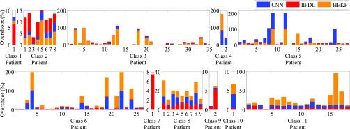
Fig. 6 presents the overshoot results by IIFDL, CNN, and HEKF for the intra-fractional variation. The measurement interval was 115.38ms, which is a middle interval of [38.46, 192.30ms]. A horizontal axis is the patient database number, and a red, blue, and orange bar indicate the overshoot value of IIFDL, CNN, and HEKF, respectively. Additionally, a black dotted line separates patient classes.
FIGURE 6.
Overshoot results for intra-fractional variation. The measurement interval is 115.38ms, which is a middle interval [38.46, 192.30ms]. The proposed IIFDL had less variation of the error values only up to 9.1%, but CNN and HEKF showed occasionally huge overshoot results almost 100%. The proposed method improved overshoot performance with higher stability in databases we utilized.
As shown in Fig. 6, the proposed IIFDL had less variation of the error values only up to 9.1%, but CNN and HEKF showed occasionally huge overshoot results almost 100%. In the same vein with the experiment of RMSE, the proposed method improved overshoot performance with higher stability in databases we utilized.
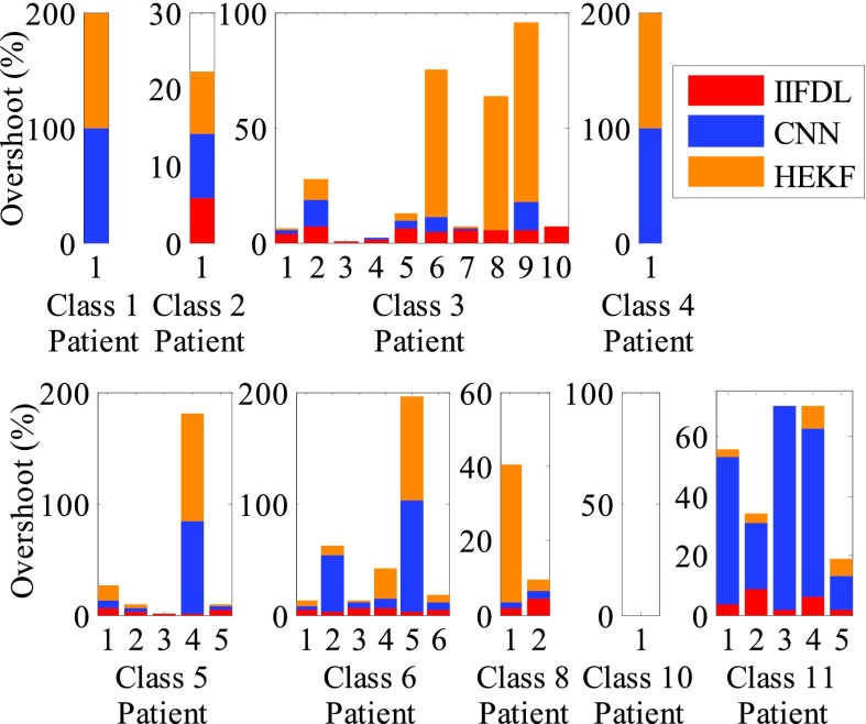
In Fig. 7, we show the overshoot results of IIFDL, CNN, and HEKF for the inter-fractional variation to demonstrate the stability of the proposed IIFDL.
FIGURE 7.
Overshoot results for inter-fractional variation. The measurement interval is 115.38ms, which is a middle interval [38.46, 192.30ms]. The maximum overshoot value of the proposed IIFDL was 8.4%. However, CNN and HEKF had large overshoot results up to 100% and wider variance of the overshoot rates than the proposed IIFDL. There was no overshoot value in Class 10.
As the experimental results of intra-fractional variation, CNN and HEKF had wider variance of the overshoot rates than the proposed IIFDL. As shown in Fig. 7, the existing methods, CNN and HEKF had large overshoot results up to 100%. However, the maximum overshoot value of the proposed IIFDL was 8.4%.
In Table 7, we summarized average overshoot rates and their standard deviation values of IIFDL, CNN, and HEKF for each measurement interval.
TABLE 7. Overshoot Comparison.
| Variation | Intra-fractional Variation (%) | Inter-fractional Variation (%) | ||||||
|---|---|---|---|---|---|---|---|---|
| Measurement Interval (ms) | 38.46 | 115.38 | 192.30 | Average | 38.46 | 115.38 | 192.30 | Average |
| IIFDL | 4.65±2.44 | 3.90±2.12 | 3.69±2.29 | 4.08±2.28 | 4.20±2.53 | 3.72±2.33 | 3.55±2.27 | 3.82±2.38 |
| Imp. Ratea over CNN [33] | 57.97 | 63.74 | 79.00 | 66.90 | 85.67 | 83.61 | 71.81 | 80.37 |
| Imp. Ratea over HEKF [32] | 78.16 | 74.12 | 72.59 | 74.96 | 90.48 | 83.97 | 84.06 | 86.17 |
Improvement Rate (Imp. Rate)  (Average of CNN/HEKF - Average of IIFDL) / Average of CNN/HEKF * 100%.
As shown in Table 7, all average overshoot rates of the proposed IIFDL are considerably lower than those of CNN and HEKF, in both experimental results for the intra- and inter-fractional variation. Furthermore, standard deviation values of the overshoot rate had remarkable differences in between IIFDL and two other methods. For the intra-fractional variation, the total standard deviation values of IIFDL, CNN, and HEKF were 2.28%, 26.78%, and 28.26%, respectively. Overall results for the intra-fractional variation showed that the proposed method improves the overshoot percentage by 66.90% for CNN and 74.96% for HEKF. For the inter-fractional variation, also, IIFDL markedly reduced not only the average overshoot percentage but also the standard deviation. The overall improvement rates of IIFDL was 80.37% for CNN and 86.17% for HEKF in the experiment for the inter-fractional variation.
3). Computing Time
To evaluate and compare effects on the computational complexity by the proposed IIFDL, we measured average CPU time of each prediction method using a PC with Intel Core i7 3.07 GHz and 16.0 GB RAM.
Table 8 compares the computing time of IIFDL, CNN, and HEKF for each measurement interval used in the experiment, where time difference represents the difference of the computing time between the previous methods and IIFDL.
TABLE 8. Computing Time Comparison.
| Variation | Intra-fractional Variation (ms) | Inter-fractional Variation (ms) | ||||||
|---|---|---|---|---|---|---|---|---|
| Measurement Interval (ms) | 38.46 | 115.38 | 192.30 | Average | 38.46 | 115.38 | 192.30 | Average |
| IIFDL | 1.32±4.91 | 1.61±5.06 | 1.70±5.07 | 1.54±5.01 | 1.32±4.91 | 1.61±5.06 | 1.70±5.07 | 1.54±5.01 |
| Time Diff.a from CNN [33] | 252.60 | 250.99 | 254.74 | 252.78 | 253.16 | 249.94 | 251.32 | 251.47 |
| Time Diffa from HEKF [32] | 251.76 | 251.47 | 252.82 | 252.02 | 250.72 | 253.36 | 249.85 | 251.31 |
Time Difference (Time Diff.)  computing time average of CNN/HEKF - computing time average of IIFDL.
In the experimental results for the intra-fractional variation of Table 8, IIFDL had the average computing time of 1.54ms and the standard deviation of 5.01ms, for all databases and intervals. The average computing time and the standard deviation were 254.32ms and 11.68ms for CNN and 253.56ms and 10.74ms for HEKF. Thus, the total average of the time difference reduced by IIFDL was 252.78ms for CNN and 252.02ms for HEKF. For the inter-fractional variation, the average computing time of the proposed IIFDL was 1.54ms and its standard deviation was 5.01ms throughput all databases and measurement intervals. The average computing time and its standards deviation were 253.01ms and 9.17ms for CNN, and 252.85ms and 6.17ms for HEKF. In the experiment for the inter-fractional variation, the total average of the time difference reduced by IIFDL was 251.47ms for CNN and 251.31ms for HEKF.
As we mentioned in Section II, the proposed FDL, requires less prediction parameters than CNN and HEKF. Accordingly, the proposed IIFDL could reduce the computing time immensely as shown in the experimental results in Table 8. Moreover, IIFDL and CNN train the multiple breathing signals simultaneously based on the respiratory feature similarities. This leads to lower the number of training process. For instance, there were 35 intra-fractional variation databases of patients in Class 2, and HEKF needed to train the respiratory signals 35 times more than IIFDL and CNN, to acquire the prediction results. Thus, the proposed IIFDL is expected to improve the prediction speed maintaining the prediction accuracy during the treatment session in the clinical perspective.
D. Comparison of Intra- and Inter -Fraction Motion
We evaluate experimental results of intra- and inter-fractional variation. Table 9 compares the two kinds of variation regarding RMSE, overshoot, and computing time.
TABLE 9. Experimental Result Comparison of Intra- and Inter-Fractional Variations.
| Variation | Intra-fractional variation | Inter-fractional variation | |
|---|---|---|---|
| RMSE | IIFDL Average (mm) | 0.33 | 0.38 |
| CNN Average (mm) | 0.97 | 0.98 | |
| HEKF Average (mm) | 0.42 | 1.01 | |
| Improvement Rate (CNN (%)/HEKF (%)) | 38.27/21.69 | 59.02/60.44 | |
| Overshoot | IIFDL Average (%) | 4.08 | 3.82 |
| CNN Average (%) | 13.14 | 21.54 | |
| HEKF Average (%) | 16.62 | 29.89 | |
| Improvement Rate (CNN (%)/HEKF (%)) | 66.90/74.96 | 80.37/86.17 | |
| Computing Time (ms) | IIFDL Average | 1.54 | 1.54 |
| CNN Average | 254.32 | 253.01 | |
| HEKF Average | 253.56 | 252.85 | |
| Time Difference (CNN/HEKF) | 252.78/252.02 | 251.47/251.31 | |
For RMSE and overshoot of the previous methods CNN and HEKF, results of the inter-fraction variation were worse than those of the intra-fractional variation as shown in Table 9. This is because the respiration variability for the inter-fraction is larger than that for the intra-fraction. On the other hand, IIFDL showed similar RMSE and overshoot results for both intra- and inter-fractional variation. Due to the reasoning capability of IIFDL for uncertainty, the proposed IIFDL achieved the similar level of the prediction results with the intra-fractional variation in the experiment for the inter-fractional variation.
In particular, average computing time was remarkable. The proposed IIFDL reduced it less than 2ms, which were over 250ms in the previous methods, CNN and HEKF. Additionally, this implies that IIFDL can be used in real-time applications as the proposed method can estimate the next respiratory signal before it comes. Specifically, the next breathing signal will come with the interval of 38.46ms to 192.30ms, and IIFDL can calculate the estimated value within 2ms on average that is before termination of the time interval.
We provide more comparison with other previous methods [6], [15], [23], [26], [32], [33] in Table 10, to verify the accuracy performance of IIFDL. The previous methods in Table 10 were referred to in Section I. As shown in Table 10, the proposed IIFDL had the lowest error results among 9 methods. However, comparability is limited as experiments were not conducted in the identical environment.
TABLE 10. Error Comparison With Previous Methods.
V. Discussion
In a curative setting, high radiation doses need to be delivered with high precision, and safety margines need to be added to the target to ensure sufficient dose coverage. However, safety margins and resulting side effects of radiotherapy compromise the ability to deliver tumoricidal treatment doses. As a result, local tumor reccurences occur in 30% of conventionally fractionated treatments [39] and less than 10% of stereotactic applications [40]. Respiratory tumor motion range and consistency vary with patient, within one fraction and between repeated fractions with change in tumor motion range >3 mm in 20% of fractions [12]. In addition to addressing intra-fractional variation, this paper also investigated prediction for inter-fractional variation that might be larger than intra-fractional variation and therefore more challenging to address [41].
Compared to currently applied population-averaged margins between 3 and ≥10 mm in motion-inclusive treatment, margins can be significantly reduced according to the residual prediction error for the individual patient using motion-tracking and IIFDL. The proposed IIFDL can contribute to treatment planning to improve delivery accuracy, by adjusting the treatment field position according to the predicted intra- and inter-fractional variation. Based on the experimental results above, we have validated that the proposed IIFDL can estimate the next breathing signal before the next incoming signal arrives. Therefore, IIFDL is expected to achieve real time prediction in a stream computing environment if the prediction system tolerates measurement delay of respiratory signal.
Future studies may seek to identify correlations between tumor location in the lung, as well as patient-related parameters and comorbidities and predicted intra- and inter-fractional variation to even further improve prediction accuracy. In addition, further study can be conducted on prediction with other machine learning methods to improve prediction accuracy of tumor motion, which have not been introduced yet for estimating intra- and inter-fractional variation, such as support vector machines [42], [43].
VI. Conclusion
In this paper, we proposed the new prediction algorithm, called FDL. Based on this algorithm, we also proposed the specific estimation method for intra- and inter-fractional variation of multiple patients, called IIFDL. Our approach has three main contributions to prediction of patients’ motion during a single treatment session and between different fractional sessions. First, the proposed method is the first study on the modeling of both intra- and inter-fractional variation for multiple patients’ respiratory data, collected from the Cyberknife facility. Second, the proposed IIFDL might enhance tumor tracking techniques due to its high prediction accuracy. Third, the proposed FDL, the predictor used in IIFDL, has a much shorter computation time than other methods, so that the proposed IIFDL shows the optimistic perspective on real-time prediction.
The experimental results validated that the RMSE value of the proposed IIFDL was improved by 38.27% of CNN and 21.69% of HEKF for the intra-fractional variation. For the inter-fractional variation, IIFDR improved the average RMSE values by 59.02% for CNN and 60.44% for HEKF. The IIFDL also improved the prediction overshoot by 66.90% for CNN and 74.96% for HEKF for the intra-fractional variation. In a case of the inter-fractional variation, the overshoot improvement was 80.37% for CNN and 86.17% for HEKF. For the average computing time, the previous methods spent over 250ms for computation, but the proposed IIFDL consumed less than 2ms. The outcomes of RMSE and prediction overshoot demonstrate that the proposed method has more of a superb prediction performance than existing approaches. Particularly, computation time results showed that IIFDL can be considered as a suitable tool for real-time estimation.
Biographies

Seonyeong Park (S’14) received the B.Eng. degree in electronics, computer, and telecommunication engineering and the M.Eng. degree in information and communications engineering from Pukyong National University, Busan, Korea, in 2011 and 2013, respectively. She is currently pursuing the Ph.D. degree in electrical and computer engineering with Virginia Commonwealth University, Richmond, VA, USA. Her research interests include machine learning, neural networks, fuzzy logic models, and target estimation.

Suk Jin Lee (S’11–M’13) received the B.Eng. degree in electronics engineering and the M.Eng. degree in telematics engineering from Pukyong National University, Busan, Korea, in 2003 and 2005, respectively, and the Ph.D. degree in electrical and computer engineering from Virginia Commonwealth University, Richmond, VA, USA, in 2012. He is currently an Assistant Professor of Computer Science with Texas A&M University–Texarkana, Texarkana, TX, USA. In 2007, he was a Visiting Research Scientist with the GW Center for Networks Research, George Washington University, Washington, DC, USA. His research interests include network protocols, neural network, target estimate, and classification.

Elisabeth Weiss received the Graduate degree from the University of Wurzburg, Germany, in 1990, the Ph.D. degree in 1991, and the Academic Teacher’s degree from the University of Goettingen, Germany, in 2004. She completed residency in radiation oncology with the University of Gottingen, Gottingen, Germany, in 1997, after participating in various residency programs in Berne (Switzerland), Wurzburg (Germany), and Tubingen (Germany). She is currently a Professor with the Department of Radiation Oncology and a Research Physician with the Medical Physics Division, Virginia Commonwealth University, Richmond, where she is also involved in the development of image-guided radiotherapy techniques and 4-D radiotherapy of lung cancer.

Yuichi Motai (S’00–M’03–SM’12) received the B.Eng. degree in instrumentation engineering from Keio University, Tokyo, Japan, in 1991, the M.Eng. degree in applied systems science from Kyoto University, Kyoto, Japan, in 1993, and the Ph.D. degree in electrical and computer engineering from Purdue University, West Lafayette, IN, USA, in 2002. He is currently an Associate Professor of Electrical and Computer Engineering with Virginia Commonwealth University, Richmond, VA, USA. His research interests include the broad area of sensory intelligence, in particular, in medical imaging, pattern recognition, computer vision, and sensory-based robotics.
Funding Statement
This work was supported in part by the National Science Foundation CAREER under Grant 1054333, the National Center for Advancing Translational Sciences through the CTSA Program under Grant UL1TR000058, the Center for Clinical and Translational Research Endowment Fund within Virginia Commonwealth University through the Presidential Research Incentive Program, and the American Cancer Society within the Institutional Research through the Massey Cancer Center under Grant IRG-73-001-31.
References
- [1].Daliri M. R., “A hybrid automatic system for the diagnosis of lung cancer based on genetic algorithm and fuzzy extreme learning machines,” J. Med. Syst., vol. 36, no. , pp. 1001–1005, Apr. 2012. [DOI] [PubMed] [Google Scholar]
- [2].Cancer Facts and Statistics. [Online]. Available: http://www.cancer.org/research/cancerfactsstatistics/cancerfactsfigures2015/, accessed Oct. 23, 2015.
- [3].Michalski D., et al. , “Four-dimensional computed tomography-based interfractional reproducibility study of lung tumor intrafractional motion,” Int. J. Radiat. Oncol., Biol., Phys., vol. 71, no. 3, pp. 714–724, Jul. 2008. [DOI] [PubMed] [Google Scholar]
- [4].Keall P. J., et al. , “The management of respiratory motion in radiation oncology report of AAPM task group 76,” Med. Phys., vol. 33, no. 10, pp. 3874–3900, 2006. [DOI] [PubMed] [Google Scholar]
- [5].Ruan D., Fessler J. A., and Balter J. M., “Real-time prediction of respiratory motion based on local regression methods,” Phys. Med. Biol., vol. 52, no. 23, pp. 7137–7152, 2007. [DOI] [PubMed] [Google Scholar]
- [6].Riaz N., et al. , “Predicting respiratory tumor motion with multi-dimensional adaptive filters and support vector regression,” Phys. Med. Biol., vol. 54, no. 19, pp. 5735–5748, Oct. 2009. [DOI] [PMC free article] [PubMed] [Google Scholar]
- [7].Nguyen C. C. and Cleary K., “Intelligent approach to robotic respiratory motion compensation for radiosurgery and other interventions,” in Proc. WAC Conf., Budapest, Hungary, Jul. 2006, pp. 1–6. [Google Scholar]
- [8].Skworcow P., et al. , “Predictive tracking for respiratory induced motion compensation in adaptive radiotherapy,” in Proc. UKACC Control Mini Symp., Glasgow, Scotland, Aug. 2006, pp. 203–210. [Google Scholar]
- [9].Sun K., Pheiffer T. S., Simpson A. L., Weis J. A., Thompson R. C., and Miga M. I., “Near real-time computer assisted surgery for brain shift correction using biomechanical models,” IEEE J. Translational Eng. Health Med., vol. 2, May 2014, Art. ID 2500113. [DOI] [PMC free article] [PubMed] [Google Scholar]
- [10].Yom S. S., et al. , “Initial evaluation of treatment-related pneumonitis in advanced-stage non-small–cell lung cancer patients treated with concurrent chemotherapy and intensity-modulated radiotherapy,” Int. J. Radiat. Oncol., Biol., Phys., vol. 68, no. 1, pp. 94–102, May 2007. [DOI] [PubMed] [Google Scholar]
- [11].Kipritidis J., Hugo G., Weiss E., Williamson J., and Keall P. J., “Measuring interfraction and intrafraction lung function changes during radiation therapy using four-dimensional cone beam CT ventilation imaging,” Med. Phys., vol. 42, no. 3, pp. 1255–1267, 2015. [DOI] [PMC free article] [PubMed] [Google Scholar]
- [12].Jan N., Hugo G. D., Mukhopadhyay N., and Weiss E., “Respiratory motion variability of primary tumors and lymph nodes during radiotherapy of locally advanced non-small-cell lung cancers,” Radiat. Oncol., vol. 10, p. 133, Jun. 2015. [DOI] [PMC free article] [PubMed] [Google Scholar]
- [13].Yan H., Yin F.-F., Zhu G.-P., Ajlouni M., and Kim J. H., “Adaptive prediction of internal target motion using external marker motion: A technical study,” Phys. Med. Biol., vol. 51, no. 1, pp. 31–44, 2006. [DOI] [PubMed] [Google Scholar]
- [14].Dhou S., Motai Y., and Hugo G. D., “Local intensity feature tracking and motion modeling for respiratory signal extraction in cone beam CT projections,” IEEE Trans. Biomed. Eng., vol. 60, no. 2, pp. 332–342, Feb. 2013. [DOI] [PubMed] [Google Scholar]
- [15].Verma P., Wu H., Langer M., Das I., and Sandison G., “Survey: Real-time tumor motion prediction for image-guided radiation treatment,” Comput. Sci. Eng., vol. 13, no. 5, pp. 24–35, Sep-Oct 2011. [Google Scholar]
- [16].Lee S. J., Motai Y., Weiss E., and Sun S. S., “Irregular breathing classification from multiple patient datasets using neural networks,” IEEE Trans. Inf. Technol. Biomed., vol. 16, no. 6, pp. 1253–1264, Nov. 2012. [DOI] [PubMed] [Google Scholar]
- [17].Huang E., et al. , “Intrafraction prostate motion during IMRT for prostate cancer,” Int. J. Radiat. Oncol., Biol., Phys., vol. 53, no. 2, pp. 261–268, Jun. 2002. [DOI] [PubMed] [Google Scholar]
- [18].Bert C. and Durante M., “Motion in radiotherapy: Particle therapy,” Phys. Med. Biol., vol. 56, no. 16, pp. R113–R144, 2011. [DOI] [PubMed] [Google Scholar]
- [19].Webb S., “Motion effects in (intensity modulated) radiation therapy: A review,” Phys. Med. Biol., vol. 51, no. 13, pp. R403–R425, 2006. [DOI] [PubMed] [Google Scholar]
- [20].Goodband J. H., Haas O. C. L., and Mills J. A., “A comparison of neural network approaches for on-line prediction in IGRT,” Med. Phys., vol. 35, no. 3, pp. 1113–1122, 2008. [DOI] [PubMed] [Google Scholar]
- [21].Langen K. M. and Jones D. T. L., “Organ motion and its management,” Int. J. Radiat. Oncol., Biol., Phys., vol. 50, no. 1, pp. 265–278, May 2001. [DOI] [PubMed] [Google Scholar]
- [22].Men C., Romeijn H. E., Saito A., and Dempsey J. F., “An efficient approach to incorporating interfraction motion in IMRT treatment planning,” Comput. Oper. Res., vol. 39, no. 7, pp. 1779–1789, Jul. 2012. [Google Scholar]
- [23].McClelland J. R., et al. , “Inter-fraction variations in respiratory motion models,” Phys. Med. Biol., vol. 56, no. 1, pp. 251–272, 2011. [DOI] [PubMed] [Google Scholar]
- [24].Gottlieb K. L., Hansen C. R., Hansen O., Westberg J., and Brink C., “Investigation of respiration induced intra- and inter-fractional tumour motion using a standard cone beam CT,” Acta Oncol., vol. 49, no. 7, pp. 1192–1198, 2010. [DOI] [PubMed] [Google Scholar]
- [25].Herk M. v., Remeijer P., Rasch C., and Lebesque J. V., “The probability of correct target dosage: Dose-population histograms for deriving treatment margins in radiotherapy,” Int. J. Radiat. Oncol., Biol., Phys., vol. 47, no. 4, pp. 1121–1135, Jul. 2000. [DOI] [PubMed] [Google Scholar]
- [26].Sharp G. C., Jiang S. B., Shimizu S., and Shirato H., “Prediction of respiratory tumour motion for real-time image-guided radiotherapy,” Phys. Med. Biol., vol. 49, no. 3, pp. 425–440, 2004. [DOI] [PubMed] [Google Scholar]
- [27].Vedam S. S., Keall P. J., Docef A., Todor D. A., Kini V. R., and Mohan R., “Predicting respiratory motion for four-dimensional radiotherapy,” Med. Phys., vol. 31, no. 8, pp. 2274–2283, Jul. 2004. [DOI] [PubMed] [Google Scholar]
- [28].Marquardt D. W., “An algorithm for least-squares estimation of nonlinear parameters,” J. Soc. Ind. Appl. Math., vol. 11, no. 2, pp. 431–441, 1963. [Google Scholar]
- [29].Putra D., Haas O. C. L., Mills J. A., and Bumham K. J., “Prediction of tumour motion using interacting multiple model filter,” in Proc. 3rd IET Int. Conf. MEDSIP, Glasgow, Scotland, Jul. 2006, pp. 1–4. [Google Scholar]
- [30].Isaksson M., Jalden J., and Murphy M. J., “On using an adaptive neural network to predict lung tumor motion during respiration for radiotherapy applications,” Med. Phys., vol. 32, no. 12, pp. 3801–3809, Dec. 2005. [DOI] [PubMed] [Google Scholar]
- [31].Murphy M. J., “Tracking moving organs in real time,” Seminars Radiat. Oncol., vol. 14, no. 1, pp. 91–100, Jan. 2004. [DOI] [PubMed] [Google Scholar]
- [32].Lee S. J., Motai Y., and Murphy M., “Respiratory motion estimation with hybrid implementation of extended Kalman filter,” IEEE Trans. Ind. Electron., vol. 59, no. 11, pp. 4421–4432, Nov. 2012. [Google Scholar]
- [33].Lee S. J., Motai Y., Weiss E., and Sun S. S., “Customized prediction of respiratory motion with clustering from multiple patient interaction,” ACM Trans. Intell. Syst. Technol., vol. 4, no. 4, pp. 69:1–69:17, Sep. 2013. [Google Scholar]
- [34].Murphy M. J., “Using neural networks to predict breathing motion,” in Proc. 7th Int. Conf. Mach. Learn. Appl. (ICMLA), San Diego, CA, USA, Jan. 2009, pp. 528–532. [Google Scholar]
- [35].Murphy M. J. and Pokhrel D., “Optimization of an adaptive neural network to predict breathing,” Med. Phys., vol. 36, no. 1, pp. 40–47, Dec. 2009. [DOI] [PMC free article] [PubMed] [Google Scholar]
- [36].Nasr M. B. and Chtourou M., “A hybrid training algorithm for feedforward neural networks,” Neural Process. Lett., vol. 24, no. 2, pp. 107–117, Oct. 2006. [Google Scholar]
- [37].Lu W., et al. , “A semi-automatic method for peak and valley detection in free-breathing respiratory waveforms,” Med. Phys., vol. 33, no. 10, pp. 3634–3636, 2006. [DOI] [PubMed] [Google Scholar]
- [38].Benchetrit G., “Breathing pattern in humans: Diversity and individuality,” Respirat. Physiol., vol. 122, nos. 2–3, pp. 123–129, Sep. 2000. [DOI] [PubMed] [Google Scholar]
- [39].Curran W. J. Jr., et al. , “Sequential vs concurrent chemoradiation for stage III non-small cell lung cancer: Randomized phase III trial RTOG 9410,” J. Nat. Cancer Inst., vol. 103, no. 19, pp. 1452–1460, Sep. 2011. [DOI] [PMC free article] [PubMed] [Google Scholar]
- [40].Timmerman R., et al. , “Stereotactic body radiation therapy for inoperable early stage lung cancer,” J. Amer. Med. Assoc., vol. 303, no. 11, pp. 1070–1076, Mar. 2010. [DOI] [PMC free article] [PubMed] [Google Scholar]
- [41].Shah A. P., et al. , “Real-time tumor tracking in the lung using an electromagnetic tracking system,” Int. J. Radiat. Oncol., Biol., Phys., vol. 86, no. 3, pp. 477–483, Jul. 2013. [DOI] [PubMed] [Google Scholar]
- [42].Daliri M. R., “Combining extreme learning machines using support vector machines for breast tissue classification,” Comput. Methods Biomech. Biomed. Eng., vol. 18, no. 2, pp. 185–191, 2015. [DOI] [PubMed] [Google Scholar]
- [43].Daliri M. R., “Chi-square distance kernel of the gaits for the diagnosis of Parkinson’s disease,” Biomed. Signal Process. Control, vol. 8, no. 1, pp. 66–70, Jan. 2013. [Google Scholar]


