Statistical iterative reconstruction using adaptive fractional order regularization

Abstract

In order to reduce the radiation dose of the X-ray computed tomography (CT), low-dose CT has drawn much attention in both clinical and industrial fields. A fractional order model based on statistical iterative reconstruction framework was proposed in this study. To further enhance the performance of the proposed model, an adaptive order selection strategy, determining the fractional order pixel-by-pixel, was given. Experiments, including numerical and clinical cases, illustrated better results than several existing methods, especially, in structure and texture preservation.

1. Introduction

X-ray computed tomography has been widely used for clinical and industrial purposes. However, the radiation risk accompanying with the increasing number of scans also draws a lot of attention [1]. The famous as low as reasonably achievable (ALARA) principle is encouraged to evade excessive radiation dose in the clinical field. Since the imaging quality is approximately proportional to the radiation dose, simply reducing the radiation dose will seriously degrade the signal to noise ratio (SNR) and the clinical values of the images.

The major methods to reduce the radiation dose can be divided into two categories: the first one is to lower the x-ray tube current or shorten the exposure time (mAs) and the second is to reduce the photon number penetrating human body. However, the former will introduce quantum noise into projection data and the later will cause sparse view, limited angle, and interior CT. In this study, we only focused on the first category of methods and the proposed model is natural to extend to other topics.

Mathematically, the procedure of CT image reconstruction can be formulated as a linear inverse problem. Both categories of the methods reducing the radiation dose will make the linear system ill-conditioned and the traditional filtered backprojection (FBP) will be powerless. In the past decades, much endeavors have been made to deal with this problem. The most classical methods include the algebraic reconstruction technique (ART) [2] and expectation maximization (EM) [3]. However, when the sampling data is highly underdetermined, both ART and EM can only achieve better results than FBP and it is still very difficult to meet the standard for clinical requirements.

Except ART and EM, other methods for the contaminated projection data can be classified into two groups in terms of objects to process. The first one is to directly process the projection data. Li et al. proposed to filter the projection data with a penalty function and solve the corresponding nonlinear system with iterated conditional mode [4]. La Rivière used the separable paraboloidal surrogates to solve a new penalized likelihood function which can obtain lower computational cost and better visual effect [5]. Wang et al. modeled the first and second moments of the noise of the projection data with a weighted least squares method and developed a penalized weighted least squares (PWLS) using the space relationship between signals as data fidelity [6]. To overcome the quasi-speckle noise and mosaic effect introduced by PWLS, Tang et al. proposed to decompose the projection data into different scales and cope with them with anisotropic diffusion [7]. Based on the spatial relations and similarity between pixels, Manduca et al. proposed a bilateral filter to process the projection data [8]. Although filter-based methods are computationally efficient and can only suppress the noise to a certain degree, it is difficult to keep the structure details very well and the artifacts introduced by the filters in the projection data will degrade the reconstructed images with unpredictable side effects.

Different from the filter-based methods, the optimization object of the second group is the image pixel. Erdogan and Fessler analyzed the statistical property of the projection data, and formulated a minimization framework including a statistical data fidelity and a regularization terms [9]. Thibault et al. applied this framework into multi-slice spiral CT [10]. Xu et al. used the classical total variation (TV) as regularization term and introduced it into interior tomography and spectral CT [11, 12]. Employing the fact that the attenuation coefficient for same material is identical, as prior information, Rashed and Kudo applied the SIR framework into sparse view problem [13]. This kind of methods has been proved to be efficient to suppress the noise and streak artifacts. The crucial part is what prior information is formulated as the regularization term and this issue is related to a popular topics - compressive sensing (CS).

Recently, compressive sensing has drawn a lot of attention in many fields. Different from the classical Nyquist–Shannon sampling theorem, CS proved that if the undersampled signal can be represented sparsely with a sparsifying transform, it can be accurately reconstructed after the corresponding inverse transform [14, 15]. The most common sparsifying transform is the discrete gradient transform and TV is the sum of the transform coefficients. Inspired by the CS theory, several methods based on TV were proposed. Sidky et al. coupled TV into projection onto convex sets (POCS) [16], derived TV-POCS for sparse and limited view problems, and extended it to circular cone-beam scan with an adaptive step-size strategy [17]. This adaptive step size strategy was improved by Ritschl et al. and the minimal value of the raw data cost function could be achieved [18]. Although TV is widely used, it has inherent flaws. TV assumes the signal is piecewise smooth, which will make the reconstructed result blocky. Meanwhile, since TV is based on the gradient of single pixel, so it is very difficult to identify the texture and edges. To overcome this problem, with similar idea, Tian et al. and Liu et al. respectively introduced a penalty weight into TV and gave an edge preserving TV (EPTV) [19] and an adaptive-weighted total variation model [20]. Several group proposed different energy model with high order regularization terms [21–23]. These energy models can efficiently eliminate the blocky effects, but new artifacts such as speckle-like noise will be introduced. Zhang et al. combined TV with a high order norm to suppress the blocky effects [24].

In the recent decades, a new mathematical tool, fractional calculus, has been applied in image processing. Different from the integer order derivative, the fractional-order derivative based TV has different frequency response characteristics corresponding to different frequency bands and can be seen as a natural inner interpolation between traditional TV and high order TV. Based on this property, fractional order derivative based models have shown their ability to mitigate the blocky effect and preserve more structure and texture information [25–33], without introducing other drawbacks such as those using the higher-order methods. More details about application of fractional calculus in signal processing can be referred in [25, 34, 35]. Pu et al. derived six numerical masks to compute the fractional order derivatives and applied them in image enhancement [25]. Bai and Feng proposed a fractional order anisotropic diffusion model and observed that when the order is 1.8 or 2.2, the best results could be obtained [26]. Zhang and Wei derived fractional bounded variation (FBV) space to restore noisy images with rich texture information [27, 28]. According to a texture detection and preservation strategy, Chan et al. presented a spatially adaptive fractional order diffusion model [29]. Zhang’s group first introduced fractional calculus into medical imaging. They proposed two energy minimization functions for CT metal artifact reduction [30, 31], and gave a fractional model for image reconstruction [32]. With these efforts, fractional calculus demonstrated powerful potential in image processing, especially, texture and structure preservation. With proper order selection, it also can mitigate the side effect caused by integer order methods, like TV and high order PDE [21–23, 36].

In this study, we proposed an adaptive fractional order selection strategy for fractional order TV and involved it into statistical iterative reconstruction framework. The numerical algorithm was given with two derivative masks. The theoretical details are described in Section 2, and the numerical and clinical experiments were provided in Section 3. Finally, the discussion and conclusion were given in Section 4.

2. Methodology

2.1 Statistical iterative reconstruction

In traditional CT system, while the x-ray beam scans the target object, part of the photons are absorbed. The remaining part will pass through the target object and be measured by the detectors. The attenuation distribution $\mu$ of the object can be calculated according to the Beer-Lambert law:

$$I=I_0\exp \left(-{\displaystyle {\int }_l\mu dl}\right),$$ (1)

where $I$ is the number of photons detected by a single detector bin along a certain path $l$ and $I_0$ is the corresponding number of photons in a blank scan.

The measured data can be described in an approximate discrete form with the Poisson distribution:

$$Y_i\sim \mathrm{Poisson}\left(b_i\exp \left(-{\displaystyle \sum _{j=1}^J{a}_{ij}{\mu }_j}\right)+r_i\right),i=1,2,\mathrm{...},I,j=1,2,\mathrm{...},J,$$ (2)

where $Y_i$ is the raw measurement along the ith x-ray path with the corresponding blank scan factor $b_i$ and read-out noise $r_i$, $A=\left\{a_{ij}\right\}$ is the system matrix, $I$ and $J$ is the total number of projections and image pixels respectively. For simplicity, we consider the monochromatic source and assume that the statistical distributions along different x-ray paths are independent. Neglecting the constant terms, the Poisson log-likelihood function which is given in [9] can be written as

$$L(\mu )=-{\displaystyle \sum _{i=1}^I\left(b_i\exp \left(-{\displaystyle \sum _{j=1}^J{a}_{ij}{\mu }_j}\right)+r_i-Y_i\log \left(b_i\exp \left(-{\displaystyle \sum _{j=1}^J{a}_{ij}{\mu }_j}\right)+r_i\right)\right)}.$$ (3)

Under the situation of low dose radiation, the reconstruction problem will become ill-conditioned and how to achieve a stable and reliable solution is still a challenging problem. Maximizing the a posteriori (MAP) is a powerful tool to deal with this problem. Then we have the following MAP function:

$$P(\mu |Y)=\frac{P(Y|\mu )P(\mu )}{P(Y)}.$$ (4)

With the monotonicity of logarithmic function and ignoring the constant term, the solution of Eq. (4) can be obtained by minimizing the following objective function:

$${\mu }^{\text{*}}=\text{arg} \underset{\mu \ge 0}{\text{min}} E(\mu )=\text{arg} \underset{\mu \ge 0}{\text{min}} \left\{-L(\mu )\text{-}\log P(\mu )\right\}.$$ (5)

With $R(\mu )\text{=-}\log P(\mu )$ and the second-order Taylor expansion for $\text{-}L(\mu )$, we can have

$$E(\mu )={\displaystyle \sum _{i=1}^I\frac{w_i}{2}{\left({\displaystyle \sum _{j=1}^J{a}_{ij}{\mu }_j}-{\hat{l}}_i\right)}^2}+R(\mu ),$$ (6)

where $w_i={(Y_i-r_i)}^2/Y_i$ is the statistical weight for the ith x-ray path and ${\hat{l}}_i$ is an estimate for linear line integral for the ith x-ray path which is defined as ${\hat{l}}_i=\log (b_i/(Y_i-r_i))$.

2.2 The proposed method

In Eq. (6), $R(\mu )$ can be seen as the prior information for the image. Originated from different image prior information, several methods have been proposed. TV is the most popular one which makes the assumption that the images are piecewise constant [36]. The method based on q-generalized Gaussian Markov field (q-GGMRF) can be seen as a generalized version for TV regularization [37]. All of these methods are local which means the numerical calculation is neighborhood-based. It is well known that this kind of methods cannot efficiently identify the complex structures and noises. The fractional order regularization has been proved powerful to deal with some fractal-like structures, such as blood vessels and superficial sulci and gyri of brain.

Here, we propose an adaptive fractional order TV regularization term and replace $R(\mu )$ in the SIR model Eq. (6)

$$\underset{\mu \ge 0}{\min }{\displaystyle \sum _{i=1}^I\frac{w_i}{2}{\left({\displaystyle \sum _{j=1}^J{a}_{ij}{\mu }_j}-{\hat{l}}_i\right)}^2}+\lambda {\Vert \mu \Vert }_{\text{AFTV}},$$ (7)

where ${\Vert \mu \Vert }_{\text{AFTV}}\text{=}{\displaystyle \sum _{j=1}^J\left|{\nabla }^{{\alpha }_j}{\mu }_j\right|}$ can be considered as an $L_1$ norm of an adaptive version of fractional order discrete gradient image ${\nabla }^{{\alpha }_j}{\mu }_j$.

2.3 The numerical scheme

There are two key parts for the numerical scheme of the proposed adaptive fractional order TV based SIR (AFTV-SIR) model. The first part is the iterative solution for our model. The second is the discretization of fractional order gradient image ${\nabla }^{\alpha }\mu$. For simplicity, we use the separable paraboloid surrogate method [9] to obtain the iterative solution for Eq. (7) as the following:

$${\mu }_j^t={\mu }_j^{t-1}-\frac{{\displaystyle \sum _{i=1}^I\left(a_{ij}{w}_i({\displaystyle \sum _{j=1}^J{a}_{ij}{\mu }_j^{t-1}}-{\hat{l}}_i)\right)}+\lambda {\frac{\partial {\Vert \mu \Vert }_{\text{AFTV}}}{\partial {\mu }_j}|}_{\mu ={\mu }^{t-1}}}{{\displaystyle \sum _{i=1}^I\frac{a_{ij}^2{w}_i}{{\gamma }_{ij}}}+\lambda {\frac{{\partial }^2{\Vert \mu \Vert }_{\text{AFTV}}}{\partial {\mu }_j^2}|}_{\mu ={\mu }^{t-1}}},$$ (8)

where ${\gamma }_{ij}=a_{ij}/{\displaystyle \sum _{j=1}^J{a}_{ij}}$ can be seen as normalized coefficients for each image pixels on a certain x-ray path, $\frac{\partial {\Vert \mu \Vert }_{\text{AFTV}}}{\partial {\mu }_j}$ and $\frac{{\partial }^2{\Vert \mu \Vert }_{\text{AFTV}}}{\partial {\mu }_j^2}$ are the first and second partial derivatives of ${\Vert \mu \Vert }_{\text{AFTV}}$ respect to $\mu$, respectively.

Then we have the iterative form for our model and now the details for how to discretize the two fractional order derivatives $\frac{\partial {\Vert \mu \Vert }_{\text{AFTV}}}{\partial {\mu }_j}$ and $\frac{{\partial }^2{\Vert \mu \Vert }_{\text{AFTV}}}{\partial {\mu }_j^2}$ will be given next.

Fractional calculus has been studied for hundreds of years. As its most important ingredient, fractional order derivatives can be viewed as a generalization of the integer order ones. The main definitions can be classified into two categories: the frequency domain ones and the time domain ones. Due to the requirement of symmetry by discrete Fourier transform, the image must be extended which will yield a high computational cost. Additionally, spatial adaptivity of the fractional order is one of the contributions of this study, so we only consider the time domain definitions. Thus, similar to [27–33], Grüwald–Letnikov fractional-order derivative was utilized to deduce the discretization version of Eq. (8).

Given a two-dimensional image$u=u_j=u_{m,n}$, where $m\in [1,M]$, $n\in [1,N]$ and $j=(m-1)\times N+n$, the discrete fractional order gradient ${\left({\nabla }^{{\alpha }_{m,n}}u\right)}_{m,n}$ at pixel $(m,n)$ is defined as

$${\left({\nabla }^{{\alpha }_{m,n}}u\right)}_{m,n}=\left({({\Delta }_x^{{\alpha }_{m,n}}u)}_{m,n},{({\Delta }_y^{{\alpha }_{m,n}}u)}_{m,n}\right),$$ (9)

where

$$\begin{array}{l}{\left({\Delta }_x^{{\alpha }_{m,n}}u\right)}_{m,n}={\displaystyle \sum _{k=0}^{K-1}{C}_k^{{\alpha }_{m,n}}{u}_{m-k,n}},\hfill \\ {\left({\Delta }_y^{{\alpha }_{m,n}}u\right)}_{m,n}={\displaystyle \sum _{k=0}^{K-1}{C}_k^{{\alpha }_{m,n}}{u}_{m,n-k}},\hfill \\ m=1,2,\dots ,M,n=1,2,\dots ,N,{\alpha }_{m,n}\in R^{+},\hfill \end{array}$$ (10)

with ${\Delta }_x^{{\alpha }_{m,n}}$ and ${\Delta }_y^{{\alpha }_{m,n}}$ being the fractional order partial derivatives of the x and y directions, $C_k^{{\alpha }_{m,n}}={(-1)}^k\Gamma ({\alpha }_{m,n}+1)/[\Gamma (k+1)\Gamma ({\alpha }_{m,n}-k+1)]$ denoting the generalized binomial coefficient, and $K$ referring to the number of pixels involved in computing the fractional order partial derivatives.

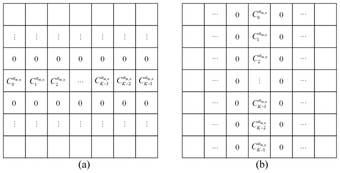
For simplicity, the computations in Eq. (10) can be considered as convolutions of the image with two shift-invariant kernels discretizing the fractional order partial derivatives. The construction for the convolution kernels can refer our previous works [32]. Figure 1 shows the concrete forms of the kernels.

Fig. 1.

Fractional-order derivative masks of (a) x and (b) y directions.

Let $M_x^{{\alpha }_{m,n}}$ and $M_y^{{\alpha }_{m.n}}$ denote the kernels we constructed in Fig. 1 and we can rewrite the calculation of Eq. (10) as

$$\begin{array}{l}{\Delta }_x^{{\alpha }_{m,n}}{u}_{m,n}=M_x^{{\alpha }_{m,n}}\ast u_{m,n},\\ {\Delta }_y^{{\alpha }_{m,n}}{u}_{m,n}=M_y^{{\alpha }_{m,n}}\ast u_{m,n},\end{array}$$ (11)

where $\ast$ is the convolution operator. With Eq. (9), we replace $u$ with $\mu$ and then have

$${\Vert \mu \Vert }_{\text{AFTV}}={\Vert {\left({\left({\Delta }_x^{{\alpha }_j}{\mu }_j\right)}^2+{\left({\Delta }_y^{{\alpha }_j}{\mu }_j\right)}^2\right)}^{1/2}\Vert }_1.$$ (12)

Let ${\upsilon }_j={\left({\left({\Delta }_x^{{\alpha }_j}{\mu }_j\right)}^2+{\left({\Delta }_y^{{\alpha }_j}{\mu }_j\right)}^2\right)}^{1/2}$, we have

$$\frac{\partial {\Vert \mu \Vert }_{\text{AFTV}}}{\partial {\mu }_j}=\frac{\partial {\upsilon }_j}{\partial {\mu }_j},$$ (13)

where

$$\frac{\partial {\upsilon }_j}{\partial {\mu }_j}=\frac{\partial {\upsilon }_{m,n}}{\partial {\mu }_{m,n}}=\frac{M_x^{{\alpha }_{m,n}}\ast {\mu }_{m,n}+M_y^{{\alpha }_{m,n}}\ast {\mu }_{m,n}}{{\xi }_{m,n}^{{\alpha }_{m,n}}}-\frac{M_x^{{\alpha }_{m+1,n}}\ast {\mu }_{m+1,n}}{{\xi }_{m+1,n}^{{\alpha }_{m+1,n}}}-\frac{M_y^{{\alpha }_{m,n+1}}\ast {\mu }_{m,n+1}}{{\xi }_{m,n+1}^{{\alpha }_{m,n+1}}}.$$ (14)

In Eq. (14), ${\xi }_{m,n}^{{\alpha }_{m,n}}=\sqrt{\epsilon +{(M_x^{{\alpha }_{m,n}}\ast {\mu }_{m,n})}^2+{(M_y^{{\alpha }_{m,n}}\ast {\mu }_{m,n})}^2}$ and $\epsilon$ is a small positive number to avoid dividing by zero. In this paper, $\epsilon$ is set to $1\times {10}^{\text{-}7}$. Following a similar way, the second order derivative of ${\Vert \mu \Vert }_{\text{AFTV}}$ can be deduced as Eq. (15):

$$\frac{{\partial }^2{\Vert \mu \Vert }_{\text{AFTV}}}{\partial {\mu }_j^2}=\frac{{\partial }^2{\upsilon }_j}{\partial {\mu }_j^2},$$ (15)

where

$$\begin{array}{c}\frac{{\partial }^2{\upsilon }_j}{\partial {\mu }_j^2}\text{=}\frac{{\partial }^2{\upsilon }_{m,n}}{\partial {\mu }_{m,n}^2}=\frac{2{({\xi }_{m,n}^{{\alpha }_{m,n}})}^2-{(M_x^{{\alpha }_{m,n}}\ast {\mu }_{m,n}+M_y^{{\alpha }_{m,n}}\ast {\mu }_{m,n})}^2}{{({\xi }_{m,n}^{{\alpha }_{m,n}})}^3}\\ +\frac{{({\xi }_{m+1,n}^{{\alpha }_{m+1,n}})}^2-{(M_x^{{\alpha }_{m+1,n}}\ast {\mu }_{m+1,n})}^2}{{({\xi }_{m+1,n}^{{\alpha }_{m+1,n}})}^3}+\frac{{({\xi }_{m,n+1}^{{\alpha }_{m,n+1}})}^2-{(M_y^{{\alpha }_{m,n+1}}\ast {\mu }_{m,n+1})}^2}{{({\xi }_{m,n+1}^{{\alpha }_{m,n+1}})}^3}.\end{array}$$ (16)

2.4 Selection of $\alpha$

In the proposed model, the selection of the fractional order $\alpha$ in image processing field is an inevitable problem. Manually choosing $\alpha$ is a common approach in most fractional models [26, 27, 30–33]. But due to the varied distribution of image features, it is difficult to reach the optimums of a globally uniform $\alpha$ with this non-intelligent strategy for every targets. It is well known that TV ($\alpha =1$) will cause staircase effect and erase some important textures. High order TV ($\alpha =2$) can efficiently suppress the blocky effect [21–23], but speckle noise will appear in cartoon regions. Based on the previous studies [28, 29, 32], it has reached a consensus that when $\alpha$ is around 1.2, the fractional order model can eliminate the staircase and speckle effect in cartoon regions and when $\alpha$ is around 1.4, the fractional order model can preserve more details in texture regions. Following the similar idea of [38] and [39], we introduced the idea of local variance and gave the formula for adaptive selection of $\alpha$ as

$$\alpha =\{\begin{array}{l}1+\frac{2}{5\pi }\text{arc tan}(P_{v_{\text{TV}}}-\min (P_{v_{\text{TV}}})),\hspace{0.17em}\text{if}\hspace{0.17em}{P}_{v_{\text{TV}}}<{\hat{\sigma }}^2\\ 1.2+\frac{4}{5\pi }\text{arc tan}(P_{v_{\text{TV}}}-{\hat{\sigma }}^2),\hspace{0.17em}\text{if}\hspace{0.17em}{P}_{v_{\text{TV}}}\ge {\hat{\sigma }}^2\end{array},$$ (17)

where ${\hat{\sigma }}^2$is the global variance of the TV residue $v_{\text{TV}}$, which is calculated as $v_{\text{TV}}=\mu -{\mu }_{\text{TV}}$. ${\mu }_{\text{TV}}$ can be obtained by smoothing the low-dose CT image reconstructed by FBP with TV filter [40]. $P_{v_{\text{TV}}}={\left(v_{\text{TV}}-\mathrm{mean}(v_{\text{TV}})\right)}^2\ast G$ is the local variance of $v_{\text{TV}}$. $G$ is a normalized symmetric Gaussian kernel, which can estimate the detail distribution in a local window. $P_{v_{\text{TV}}}<{\hat{\sigma }}^2$ can be seen as a necessary condition for cartoon regions and $P_{v_{\text{TV}}}\ge {\hat{\sigma }}^2$ for texture regions.

2.5 Overall workflow

The overall flowchart for out model is presented in Table 1.

Table 1. Main steps of AFTV-SIR.

Algorithm of AFTV-SIR
Preparation:
Obtain ${\mu }_{\text{TV}}$ by performing Chambolle-Pock algorithm [40] on the noisy reconstruction ${\mu }_{\text{FBP}}$;
Compute the residual image $v_{\text{TV}}=\mu -{\mu }_{\text{TV}}$;
Compute the global variance ${\hat{\sigma }}^2$ and local variance $P_{v_{\text{TV}}}$;
Compute $\alpha$ with Eq. (17);
Initialization:
Given, $\lambda$, $\epsilon$, $N_{ite}$, $\tau$,
Set ${\mu }^0=0$, $t=0$
Main Loop:
while $t<N_{ite}$ and $d>\tau$
Update ${\mu }^t$ with ${\mu }^{t-1}$ using Eq. (8);
$d={\Vert {\mu }^t-{\mu }^{t-1}\Vert }_2^2/J;$
$t=t+1;$
end

3. Experimental results

In this section, numerical phantom and patient data studies were performed to validate the proposed method. To further evaluate the performance of the proposed AFTV-SIR, filtered back projection (FBP), TV-SIR [11] and EPTV [19] were compared. For FBP, Ram-Lak filter was used. The parameters in TV-SIR and EPTV were set according to the suggestions in the original references [11, 19]. In this study, $N_{ite}$ was set to 1000. $\lambda$ was set to 0.3 in numerical experiment and 0.2 in patient experiment respectively. The iterative stop threshold $\tau$ was set to 0.01. The size of kernels for fractional derivatives was set to 7. The size of the normalized symmetric Gaussian kernel $S_G$ was tested in a reasonable range from 3 to 17 and $S_G$ was manually set to 9 for best reconstruction results. According to the recommendation in [38, 39], the size of the local window $S_W$ should be set to $S_W\text{=}4S_G+1\text{=37}$. It is reasonable that the optimal choice of $S_G$ is target-dependent. How to adaptively choose $S_G$ according to the image contents is out of the scope of this study and will be our future work. All the experiments were tested on MATLAB 2012b with a PC (Intel i7 4770k CPU and 8 GB RAM).

Four metrics were used in this paper for quantitative analyses. The first metric is the root mean square error (RMSE), which is defined as

$$RMSE={(({\displaystyle \sum _j{({\mu }_j-{\mu }_j^{*})}^2})/J)}^{1/2},$$ (18)

where ${\mu }_j$ is the reconstructed value, ${\mu }_j^{*}$ is the golden reference value and $J$ is the number of the pixels in the reconstructed image.

The second is the peak signal to noise ratio (PSNR), which can measure the ability of noise suppression:

$$PSNR=10\hspace{0.17em}{\log }_{10}\frac{{\left(\max ({\mu }_j)\right)}^2}{{\displaystyle \sum _j\left({\mu }_j-{\mu }_j^{*}\right)}/J}.$$ (19)

The correlation coefficient (CC) is defined as

$$CC=\frac{{\displaystyle \sum _j({\mu }_j-\overline{\mu })({\mu }_j^{*}-{\overline{\mu }}^{*})}}{\sqrt{{\displaystyle \sum _j{({\mu }_j-\overline{\mu })}^2}{\displaystyle \sum _j{({\mu }_j^{*}-{\overline{\mu }}^{*})}^2}}},$$ (20)

where $\overline{\mu }$ and ${\overline{\mu }}^{\text{*}}$ are the mean values of $\mu$ and ${\mu }^{\text{*}}$.

The structural similarity index (SSIM) was used to measure the structure similarity, which has been proved to be coherent to visual perception:

$$SSIM(\mu ,{\mu }^{*})=\frac{2\overline{\mu }{\overline{\mu }}^{*}(2{\sigma }_{\mu {\mu }^{*}}+c_2)}{({\overline{\mu }}^2+{\overline{\mu }}^{*2}+c_1)({\sigma }_{\mu }^2+{\sigma }_{{\mu }^{*}}^2+c_2)},$$ (21)

Where ${\sigma }_{\mu {\mu }^{\ast }}$ is the covariance of $\mu$ and ${\mu }^{\text{*}}$, and $c_1$ and $c_2$ are constants that we set according to [41].

3.1 Numerical phantom study

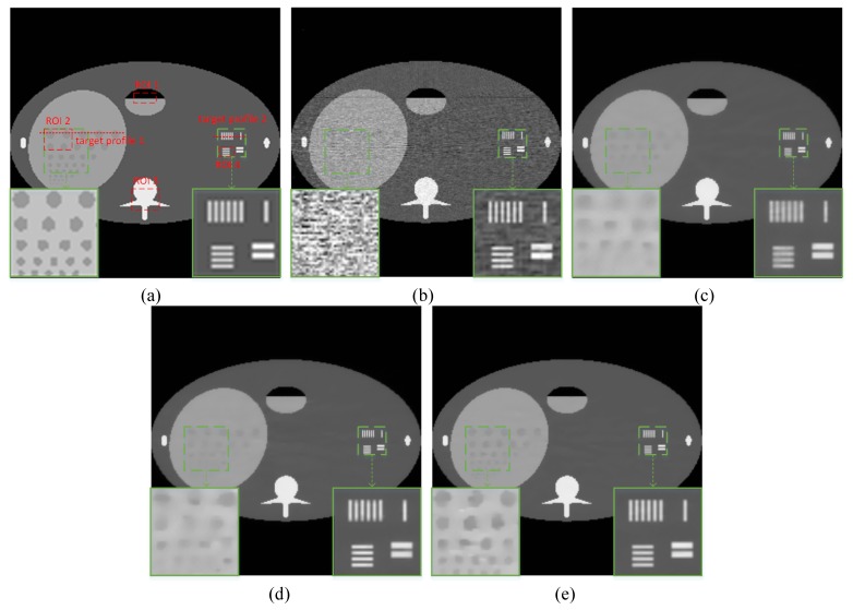
In the numerical phantom study section, the FORBILD abdomen phantom [42] which has 256 × 256 pixels, was used to test the proposed method. Siddon’s ray-driven algorithm [43] was used to simulate fan-beam geometry. The source-to-rotation center distance is 40 cm and the detector-to-rotation center is 40 cm. The image array is 20 cm × 20 cm. The detector which is 41.3 cm in length is modeled as a straight-line array of 512 detector bins. To demonstrate the performance of our method, the abdomen phantom was uniformly sampled with 300 views over 360°. After that, Poisson noise was added to each detector with photon number $b_i=5\times {10}^5$. The reconstruction results are shown in Fig. 2. It can be observed that the result from FBP contained much noise which blurred the structure information heavily, especially in the low contrast regions. TV-SIR, EPTV and AFTV-SIR suppressed most noise. However, in the zoomed low contrast and complex structure regions, which are labelled by green dotted rectangles, TV-SIR suffered from obvious blurring effect. EPTV and AFTV-SIR both obtained satisfactory resolution in the high contrast regions, but AFTV-SIR had better visual effect in the low contrast regions.

Fig. 2.

Reconstructed FORBILD abdomen phantom image for comparison. (a) Reference, (b) FBP, (c) TV-SIR, (d) EPTV, and (e) AFTV-SIR. All the images are displayed with the same window.

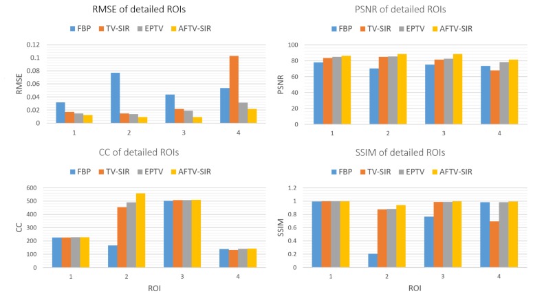
To quantitatively evaluate the performance of the proposed method, we compared theperformance of the four algorithms on the reconstruction of ROIs with detailed structures, which were marked by red dotted rectangles in Fig. 2(a). The quantitative results are given in Fig. 3. It can be seen that the AFTV-SIR obtained the best results: it has the lowest RMSE and highest PSNR/CC/SSIM for all of the ROIs.

Fig. 3.

Performance comparison of four algorithms on the reconstruction of detailed ROIs marked in Fig. 2(a) with four different indexes. The corresponding algorithms are illustrated in figure legend.

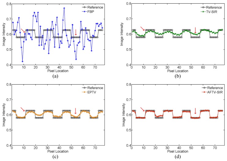
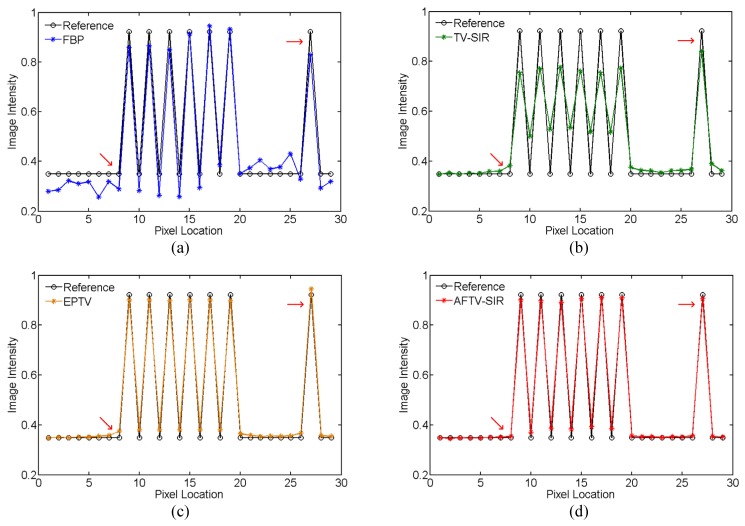
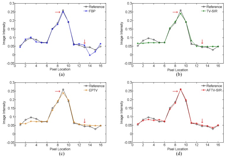
To further demonstrate the difference among the four reconstruction algorithms, two horizontal profiles of the reconstructed images were plotted across the line marked as target profile 1 and 2 in Fig. 2(a), which are respectively located in the low contrast and complex structure regions. The results further showed the advantage of three iterative algorithms over the FBP on noise suppression, as well as the advantage of the AFTV-SIR over the EPTV and the TV-SIR on edge/contrast preservation at the matched noise level (see Figs. 4 and 5).

Fig. 4.

Comparison of the target profile 1 marked in Fig. 2(a) for different methods.

Fig. 5.

Comparison of the target profile 2 marked in Fig. 2(a) for different methods.

AFTV-SIR had the best profile matching with the reference than other methods, evidenced by red arrows in Figs. 4 and 5.

3.2 Patient data study

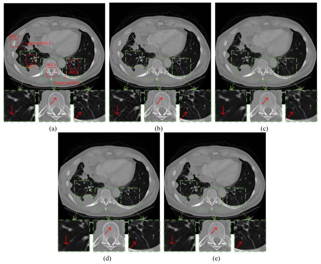
In this study, we used CT images collected on a GE Discovery CT 750 HD Scanner. We specified a representative slice from the image volume to evaluate our methodology. The image is of 256 × 256 pixels. The tube voltage was set to be 120 kVp, and the mAs level was 100 mAs. We regarded this acquisition as the normal-dose scan, and for the consideration of radiation dose, we simulated the corresponding low-dose projection data by adding noise to the normal-dose projection data using the same method in the previous subsection. The photon number was set as $b_i=5\times {10}^5$. The projection geometry was the same as that of the numerical phantom study part. To demonstrate the capability of the proposed method for low dose reconstruction, 1160 views were collected, and they were uniformly distributed over a full scan range. The reconstruction results were shown in Fig. 6, where (a) and (b) are the FBP reconstructed images from the acquired normal-dose and simulated low-dose projection data, respectively. Figure 6(c), 6(d), 6(e) are the reconstructed images from the simulated low-dose projection by the TV-SIR, the EPTV, and the AFTV-SIR algorithms. It can be observed that TV-SIR, EPTV and AFTV-SIR eliminated most of the noise. However, blocky effect can be seen in Fig. 6(c) and some tiny structures were blurred. In the zoomed parts labeled by green dotted rectangles, AFTV-SIR preserved more details than TV-SIR and EPTV and efficiently suppressed the blocky effect, indicated by the red arrows.

Fig. 6.

Reconstructed patient image for comparison. (a) Reference, (b) FBP, (c) TV-SIR, (d) EPTV, and (e) AFTV-SIR. All the images are displayed with the same window.

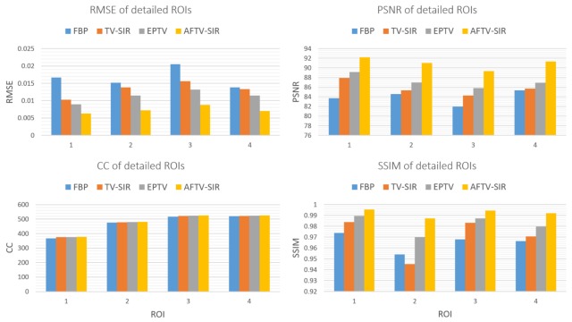
To quantitatively evaluate the performance of the proposed method we compared the performance of the four algorithms on the reconstruction of ROIs with detailed structures, which were marked by red dotted rectangles in Fig. 6(a). The quantitative results (Fig. 7) have the similar trend as the phantom study. The AFTV-SIR had the lowest RMSE and the highest PSNR/CC/SSIM for all of the ROIs.

Fig. 7.

Performance comparison of four algorithms on the reconstruction of detailed ROIs marked in Fig. 5(a) with four different indexes. The corresponding algorithms are illustrated in figure legend.

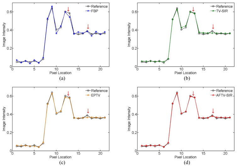
Also two vertical profiles were chosen from two different regions, which represented high contrast structure (bone) and low contrast structure (vessel) respectively. The results plotted in Figs. 8 and 9 obviously showed that iteration-based methods could achieve better results on noise suppression, but TV and EPTV could also smooth structures in the low frequencyregions which is labelled by red arrows. AFTV-SIR obtained better matching performance on both structure and contrast preservation.

Fig. 8.

Comparison of the target profile 1 marked in Fig. 5(a) for different methods.

Fig. 9.

Comparison of the target profile 2 marked in Fig. 5(a) for different methods.

4. Discussions and conclusion

SIR framework has been proved to be a powerful tool to deal with quantum noise caused by lowering the x-ray tube current or shortening the exposure time. The selection of the regularization term is flexible and will prominently impact the performance of noise suppression. TV is used as the most common regularization term, which has shown its ability to eliminate the noise. However, due to the congenital defect of mathematical assumption, TV suffers from blocky effect, which means small details, including edges and structures are smoothed. And these details in medical images might indicate some primary nidi, which would have important clinical value. In this study, a generalized version of TV called as fractional order TV was coupled into the SIR framework to overcome the blocky effect. In addition, an adaptive strategy for order selection was given to further improve the performance of this method. In both numerical and clinical cases, our method achieved better results than TV-SIR and its variant EPTV on detail and contrast preservation. The essence of the proposed method is the fractional order TV term. It was shown that, by adjusting the fractional order, the fractional order based TV model could efficiently eliminate the blocky effect and preserve more details. We measured the structure characteristics of each pixel with a statistical variable defined as local variance and introduced it into the computation of the fractional order. When the region belonged to cartoon, the order was small. Once the regions have more details, the order rose.

The selection of the parameter $\lambda$ is a vital factor to impact the performance of the regularization based method. Due to the case dependence of $\lambda$, we only chose $\lambda$ manually to balance the tradeoff between regularization and fidelity terms to obtain the best imaging quality. There has been some methods to choose $\lambda$ according to the noise property in image domain [38, 39]. However, the noise in CT images only obey some certain distribution in projection domain, not in image domain. In future, we would study a parameter selection method to ensure an approximate optimal solution for the reconstruction.

Another issue we must mention here is the computational cost. Iterative reconstruction methods suffer from heavy computational burden for the loops of re-projection and backprojection operations between image and projection domains. The proposed AFTV-SIR has a same computational complexity as TV-SIR. The main expense is blamed on the convolution operation with the proposed kernels of fractional order derivative. From a mathematical point of view, decreasing the size of the mask would be a possible way to reduce the computational cost, but the accuracy of fractional order derivative would be sacrificed. In practice, the extra computational expense can be alleviated by several methods. One possible software approach is ordered subset method, which can be recognized as a parallelization of computational operations. Another popular way is to code based on the graphics processing unit (GPU). Many studies have shown the possibility of GPU to dramatically accelerate the iterative procedure [44, 45]. With these powerful tools, iteration-based reconstruction methods will be very close to clinical applications.

In this study, our effort focused on the noise suppression for low-dose CT. The proposed regularization item had power to be involved into other energy minimization function based imaging topics. In the future, we can extend the proposed method to other topics in medical imaging, including sparse view reconstruction, interior reconstruction, limited view reconstruction, metal artifact reduction, etc.