The Great Recession and Mother’s Health

Abstract

We use longitudinal data from the Fragile Families and Child Well-being Study to investigate the impacts of the Great Recession on the health of mothers. We focus on a wide range of physical and mental health outcomes, as well as health behaviors. We find that increases in the unemployment rate decrease self-reported health status and increase smoking and drug use. We also find evidence of heterogeneous impacts. Disadvantaged mothers—African-American, Hispanic, less educated, and unmarried–experience greater deterioration in their health than advantaged mothers—those who are white, married, and college educated.

The Great Recession in the U.S. was deeper and longer than any previous recession since the 1930s. From peak – December 2007- to trough -June 2009-, output contracted by 4%, the employment rate fell by 6.3%, and the unemployment rate went from 4.8% in April 2008 to 10.6% at its peak in January 2010 (NBER, at 〈http://www.nber.org/cycles.html〉). As of June 2013, the unemployment rate was still 2.8 percentage points above what it was at the start of the recession, the labor force participation rate was 63.5%, the lowest rate since 1978, and the percentage of the population with a job, 58.7%, was stuck near levels last seen in the early 1980s (Bureau of Labor Statistics, 2013; Center for Budget Policy and Priorities, 2013).

The start of the Great Recession was severe, sudden, and sharp, and many people experienced some form of financial, psychological, or physical strain. New evidence on the effects of the Great Recession has confirmed that losses were disproportionately concentrated among minorities, youth, low income, and less-educated workers (Grusky et al., 2011; Hoynes et al., 2012), and that while men have faced higher unemployment than women, their employment recovery has been faster (Kochhar, 2011).

Since the Great Recession represented a huge financial and psychological shock for many households, and in particular for the most vulnerable, it may have had a significant impact on people’s health. Many studies have examined the relationship between economic downturns and health outcomes; however, the conclusions are mixed. This study aims to contribute to this discussion by investigating the impacts of the Great Recession on the physical and mental health and health behaviors of women with children.

Our study contributes to the literature in several ways. First, we are one of the first studies to use longitudinal data to analyze the effects of economic fluctuations on health, and the first to do so for the case of the Great Recession. We employ panel data from the Fragile Families and Child Well-being Study (FF) that allows us to observe the same mother before and during (the start of) the financial crisis, so we are able to control for individual time-invariant characteristics that might be correlated with both the probability of residing in an area with high unemployment and with experiencing declines in health. Second, by including data that incorporates the Great Recession (from mid-2007 to the beginning of 2010), we are able to exploit greater exogenous variation in the unemployment rate across states and years, as compared to studies using pre-Great Recession data that have examined macroeconomic downturns that exhibit less variation and shorter unemployment durations. Third, we focus on mothers. Most evidence regarding the link between economic fluctuations and health has focused on employed workers (usually men), who have traditionally had the strongest labor force attachment. Hence, much less is known about mothers who have varying degrees of labor force participation but may also be impacted by high unemployment in their communities. Focusing on mothers is especially interesting given recent research showing that inequality starts early in life and that the children of disadvantaged mothers are more likely to grow up to be disadvantaged themselves (Almond and Currie, 2011; Case et al., 2005; Currie, 2009; Currie and Stabile, 2003). Fourth, the FF provides a wide range of self-reported health outcomes – including measures of physical and mental health as well as health behaviors. Fifth, we examine heterogeneity of response by race/ethnicity, education, and family structure.

We find that the crisis worsened mothers’ self-reported health status and led to increases in their smoking and drug use. We also find heterogeneous responses. Blacks and Hispanics, unmarried women, and mothers with a high school degree or less became less likely to report “excellent” or “very good” health or to have good mental health; whites, married women, and highly educated mothers on the other hand, were likely to have better mental health as well as to experience some improvements in their physical health: whites were less likely to be obese and highly educated women were less likely to have health problems as unemployment increased. In other words, our results confirm that the Great Recession helped accentuate health disparities between mothers in more and less advantaged families, a result that may have disturbing implications for future disparities between their children.

This paper is organized as follows: section 1 presents a summary of the related literature, sections 2 and 3 describe the data and the empirical strategy, respectively, followed by the results in section 4 and some extensions in section 5. Section 6 provides a brief conclusion.

1. Background

Previous studies of the effects of economic shocks on health have come to very different conclusions. A number of studies claim that health improves during economic downturns, arguing that this is largely because people change their health behaviors (e.g., smoke and drink less, lose weight, exercise more, etc.) (e.g., Dehejia and Lleras-Muney, 2004; Ruhm, 2000, 2003, 2005; Ruhm and Black, 2002). Other studies find that unemployment is associated with poorer health, a finding that is variously attributed to the stress associated with losing a job, fearing job loss, and/or reductions in income and wealth (Browning and Heinesen, 2012; Dee, 2001; Eliason and Storrie, 2009a,b; Sullivan and Wachter, 2009). The lack of consensus and the fact that most of the evidence pertains to prime-age men suggest that additional research is warranted.

Table 1 provides an overview of the previous literature. Most prior work utilizes repeated cross sections of U.S. data, often at the state level, and exploits state and year variation in the unemployment rate to examine changes in health and health behaviors. Previous studies have also concentrated on analyzing health outcomes for working-age individuals with strong labor force attachment, usually men. Thus, little is known about the impact of unemployment on other demographic groups (e.g., mothers). Almost all studies predate the Great Recession.

Table 1.

– Effects of UR on Health Outcomes

OUTCOME VARIABLE
Study and Data	Health status/Health problem that limits work	Weight	Use of medical care / Health insurance	Smokes	Drinks	Mental health
1. Studies Examining Men and Women
Ruhm (2000) Micro Data: -BRFSS: 1987–1995 N =114,000 men and women Methods: Linear model		A 1pp rise in the UR reduces: -Underweight by 0.06pp -Overweight by 0.17pp -Obesity by 0.21pp No analysis by gender	A 1pp rise in the UR reduces: -Visits to the doctor by 0.57pp No analysis by gender	A 1pp rise in the UR: -Reduces smoking by 0.3pp -Reduces # of cigs per day by 0.8pp for current smokers No analysis by gender	A 1pp rise in the UR: -Increases alcohol consumption but is NON-significant No analysis by gender
Ruhm and Black (2002) Micro Data: -BRFSS: 1987–1999 -N = 500,000 men and women Methods: Linear model					A 1pp rise in UR: -Reduces predicted drinking by 0.2pp -Reduces log(# of drinks) in last-month by 3.1pp for drinkers -No effect on binge drinking By gender: -No difference in the probability of drinking -Higher decline for men: # of drinks falls by 3.4pp versus 2.8pp for females
Ruhm (2003) Micro Data: -NHIS: 1972–1981 for individuals 30+ 3 samples: Full sample: N =217,471 men and women 30–64-year-old workers: N = 115,463 obs, men and women 30–55-year-old working males: N = 57,633 Methods: Linear model	A 1pp fall in the UR: -For everyone: increases the probability of having a medical condition (chronic or acute) by 0.6pp -Stronger effects for men of working age By gender: -For men 30–55: increases by 0.63pp -For women 30–55: increases by 0.59pp		Hospital visit is NON-significant in all cases A 1pp fall in the UR: -For everyone: the probability of hospitalization falls by 0.11pp and doctor visits rises by 0.3 although NON-significant -Stronger effects for men of working age By gender results were non-significant: -For men 30–55: falls by 0.11pp -For women 30–55: falls by 0.13pp
Ruhm (2005) Micro Data: -BRFSS: sample includes individuals aged 18+ from the 1987–2000 waves N = approx. 1.5 million obs, men and women Methods: Linear model		-A 1pp fall in the employment rate: -Reduces obesity by 0.07pp -Reduces severely obese by 0.4pp -No effect on overweight No differences by gender		-A 1pp fall in the employment rate reduces: -Smoking by 0.13pp -Smoking of at least 20 cigs/day by 0.10pp smoking at least 40 cig/day by 0.015pp By gender: The effect on smoking is stronger for females (0.17pp) than for males (0.09pp)
Dee (2001) Micro Data: -BRFSS, 1984–1995 -N > 700,000, ‘prime-age’ men and women 18+ (average age is 45) Methods: Linear model					A 5pp increase in UR: -Reduces drinks per month by 3.5% and chronic drinking participation (60 or more drinks/month) by 19% -Binge drinking rises by 8% By gender: -The probability of binge drinking for males is >3 times larger than that for females
Tekin, McClellan, and Minyard (2013) Micro Data: -BRFSS Sample: N=849,594, individuals in the Labor force, ages 25–55 Methods: Linear model	A 1pp drop in ER: -Probability of being in poor health rises by 0.00067 pp (4.8%) By gender: -Strongest effects on females: “excellent health” falls by 0.0044pp (1.8%) and poor health increases by 0.0015pp(1.0%)				A 1pp drop in ER: -Binge drinking (respondent reports had 60 or more drinks during the past month) falls by 0.0023pp By gender: -Effect on binge drinking is driven by women (0.0022pp)
2. Studies Examining Men Only
Charles and DeCicca (2008) Micro Data: -NHIS: Sample of working-aged men in the US living in “large” MSAs: 1997–2001 N=30,000–35,000 men of working age Methods: Linear model		A 1pp rise in the UR: -Men with low ex-ante employment probabilities experience an increase in underweight by 0.5pp, in overweight by 3.5pp, and in obesity by 2.pp No effects on men with high employment probability		A 1pp rise in the UR: -Smoking rises by 2.7pp for those in the lowest employment decile -2.3pp reduction for those most likely to be employed	A 1pp rise in the UR: -Only for the group with highest employment probability drinking rises (3.6pp) -# of days with 5 drinks or more declines for all but it is not statistically significant	A 1pp rise in the UR: -Leads to rises in: sadness (1.5pp), hopelessness (1.1pp), worthlessness (0.9pp), restlessness (1.2pp), nervousness (1.3pp), and feelings of effort (2.5pp) -Strongest effects for those least likely to be employed
Xu and Kaestner (2010) Micro Data: -BRFSS (1984–2005, N=506,753) and NHIS (1976–2001, N=216,113), men between 25–55 Methods: Linear model			A 2.5% increase in employment: -Decreases doctor visits by 1.5pp	A 2.5% increase in employment: -Increases smoking by 1 pp -Increases smoking intensity (smokes >19 cigarettes a day y/n) by 2pp	A 2.5% increase in employment: -Increases drinking by 0.1pp -Decreases binge drinking by 0.2pp
3. Sample: Longitudinal data
Davalos and French (2011) Micro Data: -NESARC, PANEL, 2001/2002 and 2004/2005, men and women, ages: 18–59, prop. employed 78%; N = 26,313 Methods: Linear model, individual fixed-effects	A 1% increase in UR: OLS: -non-significant effects on physical health score Individual FE: -reduces physical health score by 0.9% No differences by gender					A 1% increase in UR: OLS: -reduces mental health score by 1.3% Individual FE: -reduces mental health score by 1.2% No differences by gender
Davalos, Fang, and French (2012) Micro Data: -NESARC, PANEL, 2001/2002 and 2004/2005, men and women, ages: 18–59, prop. employed= 64%; N = 34,120 Methods: -Logit, logit individual fixed-effects					A 1pp increase in state UR: Individual-FE: -Leads to a 1 binge drinking day increase per year -A 1.350 increase in the odds of driving after too much drink -A 1.167 increase in the odds of alcohol abuse/dependence No differences by gender (not shown)

1.1. How Could the Unemployment Rate Affect Health?

In a pioneering study, Ruhm (2000) linked data on state unemployment rates with state-level Vital Statistics mortality records from 1971 to 1992, to examine the link between economic downturns and mortality. He found that a 1 percentage point increase in the state unemployment rate was associated with a 0.5% reduction in state mortality rates, and he claimed that this result was mainly driven by men of working age.² Ruhm (2003), Neumayer (2004), and Gerdtham and Ruhm (2006), all find that higher unemployment is associated with lower mortality, and that individuals are less healthy during economic expansions. Dehejia and Lleras-Muney (2004) found that infant health improves in times of high unemployment.³ However, Miller el al., (2011) suggest that cyclical changes in mortality are concentrated in the young and old, and so are unlikely to primarily represent changes in health behaviors among working age adults.

In contrast to most studies using aggregate data, studies using individual-level data tend to find negative effects of unemployment on health. For example, Sullivan and Wachter (2009) use administrative data to follow a large sample of individuals subjected to mass layoffs in Pennsylvania and find significantly higher mortality due to accidents and heart conditions. These findings have been confirmed in two studies using Swedish data (Eliason and Storrie 2009a,b), and in a study using Danish data (Browning and Heinesen, 2012).

The disconnect between the literature on the effects of individual job loss and the literature on the effects of unemployment on state-level outcomes suggests that it may be fruitful to investigate the effects of unemployment using individual-level longitudinal data, as we do in this paper.

1.2. How Does the Unemployment Rate Affect Health-Behaviors?

While Ruhm (1995) and Ruhm and Black (2002) found that drinking is pro-cyclical, Ruhm (2000) later found that the association between the state unemployment rate and binge drinking was positive, although non-significant and Tekin, McClellan, and Minyard (2013) found a negligible impact. Charles and DeCicca (2008), Xu and Kaestner (2010), Dee (2001), and Deb et al., (2011) provide evidence that drinking increases significantly during recessions⁴.

The evidence on smoking is even less conclusive. While a number of studies have found that when the economy contracts, smoking declines (Ruhm, 2000, 2005; Xu and Kaestner, 2010), others find that smoking is counter-cyclical (Dehejia and Lleras-Muney, 2004), or that there is a differential impact across demographic groups. Charles and DeCicca (2008) found that smoking was counter-cyclical for minority and less educated men, whereas for those most likely to be employed, smoking fell in times of high unemployment.

Studies of the effect of economic fluctuations on obesity –a well-established risk factor for cardiovascular disease, high blood pressure, and diabetes – provide similarly ambiguous findings. While Ruhm (2000, 2005) argues that during recessions body mass index (BMI) declines significantly and is particularly driven by those with severe obesity, Charles and DeCicca (2008) and Deb et al., (2011) found an increase in obesity that seemed to be driven by minority and less educated groups.

Studies have also found a strong correlation between individual job loss and clinical and subclinical depression, anxiety, and substance use (Murphy and Athanasou, 1999). Several economic studies argue that as the unemployment rate rises, mental health worsens, and that this is evident in outcomes such as suicides and suicide attempts (Browning and Heinesen, 2012; Ruhm, 2000); anxiety, depression, loss of confidence, and self-esteem (Theodossiou, 1997); feelings of sadness, hopelessness, worthlessness, restlessness, and nervousness (Charles and DeCicca, 2008); and substance use (Dee, 2001).

Nevertheless, Tekin, McClellan, and Minyard (2013) find that only better educated individuals experience more mental health problems, and they argue that economic deterioration exacts a larger toll on individuals who have a higher opportunity cost of job loss. Other studies have shown that experiencing unemployment is more strongly associated with mental health problems in men than in women (Artazcoz et al., 2004).

Only two studies use U.S. longitudinal data to examine the effects of recessions on health.⁵ Davalos and French (2011) and Davalos, Fang, and French (2012), focus on the period 2001 to 2005 and conclude that increases in the state unemployment rate led to a decline in physical and mental health, and to a rise in drinking among male and female workers aged 18 to 59. However the effects were rather small, which may reflect the fact that the 2001 recession was mild and of short duration (Kliesen, 2003), providing little variation in unemployment rates.

1.3. Why the Effects of Unemployment Rates Are Likely to Be Heterogeneous?

There are several reasons why we expect to find heterogeneous effects of the unemployment rate on different groups of mothers. First racial and ethnic minorities, less-educated, and younger workers experience higher unemployment and more pronounced income declines during recessions than other workers (Hoynes et al., 2012; Kochhar et al., 2011; Pfeffer et al., 2013; Sierminska and Takhtamanova 2011; Verick, 2010). Indeed, many families are not at risk of unemployment and some may even profit from recessions.

Second, disadvantaged women are more likely to work in low quality jobs with precarious work environments, nonstandard work hours, and low job satisfaction and are subject to higher physical and mental health risks, and lower access to health insurance (Fischer and Sousa-Poza, 2009; Kim et al., 2008). In addition to being more vulnerable to changes in economic conditions, these mothers experience higher poverty, and poverty has been associated with less preventive health care and poorer overall health (DiMatteo et al., 2002; Katz and Hofer, 1994). In addition, poverty impedes cognitive function and so when the poor face monetary concerns during times of high unemployment, they may lose their capacity to give full consideration to other problems, including health issues (Mani et al., 2013). Moreover, cumulative socioeconomic disadvantage can have negative effects on physical health (Geronimus, 1992).

Finally, we expect larger effects of unemployment on unmarried as compared to married mothers. Unmarried mothers are significantly more likely to be African-American or Hispanic and are more disadvantaged in terms of their education, income, and assets and wealth—all of which make them more vulnerable to labor market fluctuations and which also limit their capacity to buffer shocks. Over and above these disadvantages, unwed mothers are disadvantaged by having to be both primary breadwinners and primary caretakers of their families and by their lower capacity to insure against contingencies and to risk share within the household (Becker, 1981; Lam, 1988). Unmarried mothers are likely to experience more stress, which could exhaust and undermine their health (Acs and Nelson, 2004; Ross and Van Willigen, 1996).

As this summary indicates, the evidence on the relationship between economic fluctuations and health is far from clear. The heavy reliance on repeated cross-sections, aggregate data, lack of variation in unemployment rates in the few longitudinal studies, and insufficient attention to possibly heterogenous impacts of unemployment are weaknesses of the existing literature. Moreover, most of the existing evidence pertains to prime aged men. This study will add to the literature by using longitudinal data, incorporating the dramatic increase in unemployment caused by the Great Recession, and by attending to possibly heterogeneous effects.

2. Data

To investigate the impacts of the Great Recession on mother’s health, we employ the Fragile Families and Child Wellbeing Study (FF), a longitudinal study of 4,897 births that occurred in 20 large U.S. cities (population of 200,000 or more) located in 15 states, between 1998 and 2000. Unmarried couples were oversampled and constitute about three fourths of the data. When weighted, the sample is representative of births in each of the 20 cities (a smaller sample is representative of urban births in all American cities with populations over 200,000. The mean values of variables reported are similar in the two samples). Mothers and fathers were interviewed in the hospital shortly after the birth of the focal child, and follow-up interviews were conducted when the focal child was approximately 1, 3, 5, and 9 years old (waves 2, 3, 4, and 5 respectively).

The FF data are uniquely suited to looking at the short term effects of the Great Recession, as the most recent data collection, year 9, occurred between May 2007 and February 2010. We pooled years 5 and 9 (periods 2003–2005 and 2007–2010, respectively), which are the years before and after the beginning of the Great Recession. Of the almost 5,000 mothers interviewed at baseline, 4,350 were interviewed at year 5, and 3,515 at year 9. Of these 3,500 mothers, a substantial proportion (2,003 women who represent 57% of the sample in year 9) was interviewed in 2009–2010, right at the peak of the financial crisis. We focus on these last two waves of data (and exclude years 1 and 3) for two reasons. First, we are interested in examining the impacts of the Great Recession on mother’s health. Second, not all health outcomes were available for all waves.⁶ After restricting the sample to these two waves and to women with complete information on the outcome variables, our analytic sample includes approximately 3,500 mothers (the N varies by the outcome measured).⁷ We investigate possible differential attrition further below.

The outcomes of interest for this study include eight measures of self-reported physical and mental health, and health behaviors that were obtained from telephone or in-home interviews, and refer to the last 12 months.⁸ All measures were constructed as binary indicators that take the value of 1 when a mother reports that she has a given condition and 0 otherwise. We construct binary variables since most of the health questions in the questionnaire ask a mother to either provide a yes/no answer or a categorical response. For the cases in which we have continuous variation in a mother’s health outcome (i.e., body mass index), we also explore the association between this outcome and economic conditions. These results are shown in the Extensions section. The following list describes each of the outcomes we investigate:

Physical health

• 1)Self-rated health status: “excellent” or “very good” health status versus “good”, “fair”, or “poor”.
• 2)Health problem that limits work: has a health problem that limits work or study-related activities versus no problem.
• 3)Obesity: mother’s BMI is equal to or more than 30 versus BMI less than 30.
• 4)Health insurance: covered by either a private insurance or Medicaid versus no insurance.

Health Behaviors

• 5)Smokes: smokes cigarettes versus no smoking in the last month.
• 6)Binge drinking: drinks 4 or more glasses of alcohol in one occasion versus less than 4 glasses in 1 occasion or no drinking, in the last year.
• 7)Drug use: uses one or more drugs (includes illegal drugs, sedatives, tranquilizers, amphetamines, or other)⁹ “on your own”, versus no drug-use. By “on your own” is meant either without a doctor’s prescription, in larger amounts than prescribed, or for a longer period than prescribed.

Mental health

• 8)Depression (screener): respondent could be potentially assessed as depressed¹⁰ versus not depressed.

Although these eight measures are self-reported and have not been medically verified, they have been widely used in previous studies of population health and have been found to be highly correlated with medically determined health status (Currie and Madrian, 1999; Miilunpalo et al., 1997). Also, the mental health outcome we use in this study is a robust screener for the likelihood of experiencing a psychiatric condition known as a major depressive episode (Kessler et al., 1998). This outcome is constructed based on the short form of the World Health Organization Composite International Diagnostic Interview (CIDI-SF) which has been commonly used in large-scale community surveys to measure depression (Aalto-Setälä et al., 2002).¹¹

We expect that these measures of health could respond to changes in economic conditions that have occurred in the last 12 months, since previous studies have shown that physical and mental health and health behaviors are sensitive to short-term changes in unemployment (i.e., monthly UR) (Charles and DeCicca, 2008; Ruhm, 2005; Ruhm and Black, 2002). Even more stable health outcomes like obesity could change over the period of one year when one considers that BMI could change enough to cause the person to cross the obesity threshold (see column 2 in Table 1). In the particular case of smoking, although it is true that few people start smoking after age 25, people can re-start smoking after this age, and this is actually relatively common. For example, among mothers in FF, we find that 6% of sample has re-started smoking in year 9 after years of non-smoking.

From the perspective of a health production function (Grossman, 1972), it is also reasonable to expect that changes in economic conditions could affect individual health investments as they could have an impact on wages, income, or on the opportunity cost of time, which in turn could lead to changes in overall health. Moreover, if we take into account that the Great Recession was deeper and longer than other recessions previously analyzed, it is also reasonable to expect that more dramatic changes in the UR are more likely to be associated with changes in health.

2.1. Mother Characteristics and Health outcomes

Table 2 presents weighted summary statistics for all the women in the sample, and by race/ethnicity. Descriptive statistics indicate that 62% of the sample report health that is “excellent” or “very good”, 10% have a problem that limits their work or study activities, a third are obese, and only 81% are covered by health insurance. In terms of health behaviors, 30% of the mothers smoke, 13% drink more than 4 glasses of alcohol on one occasion (binge drink), and 5% report drug use “on their own.” Almost 15% of the mothers show depressive symptoms on the screener. Comparable figures from the Center for Disease Control and Prevention (2012) indicate that 55% of women in the U.S. have “excellent” or “very good” health (whites 65%, blacks 48%, and Hispanics 51%), 30% are obese, 84.4% are covered by health insurance coverage, 17% smoke cigarette, 12% binge drink each month, and 11% had at least one major depressive episode (including depressed mood and markedly diminished interest or pleasure in all, or almost all, activities) in the past year.^12,13 These numbers suggest that FF women have on average better or similar physical health to the average US woman, worse mental health, and higher risk health behaviors¹⁴.

Table 2.

Summary Statistics in FF

Variable	Full	Whites	Blacks	Hispanics	UR>6%	UR<=6%
Health outcomes: Health Excellent/V. Good a b	0.612	0.750	0.547	0.530	0.607	0.613
Health Limits Work a b c	0.103	0.072	0.130	0.113	0.106	0.101
Obesity a b c d	0.320	0.195	0.402	0.386	0.348	0.302
Any health Insurance a b c d	0.809	0.910	0.861	0.640	0.793	0.820
Smokes a b c	0.302	0.369	0.338	0.199	0.295	0.307
>=4 Drinks 1 Time Last Yr. a b c	0.126	0.206	0.083	0.108	0.126	0.127
Drugs use b c d	0.053	0.063	0.063	0.039	0.062	0.046
Depressed a c	0.132	0.128	0.147	0.130	0.132	0.132
Race/ethnicity: White d	0.284	1.000			0.265	0.298
Black	0.357		1.000		0.351	0.361
Hispanic d	0.290			1.000	0.308	0.276
Other race	0.070				0.077	0.065
Immigrant b c d	0.239	0.073	0.075	0.460	0.263	0.221
Education: <HS a b c d	0.271	0.116	0.286	0.455	0.284	0.262
HS a b c	0.329	0.219	0.436	0.320	0.327	0.331
Some college a b c	0.203	0.207	0.236	0.173	0.210	0.197
College or > a b c d	0.197	0.457	0.042	0.053	0.180	0.211
Marital Status: Married a b c	0.519	0.818	0.231	0.502	0.517	0.520
Cohabiting a b c	0.233	0.114	0.297	0.309	0.234	0.233
Single a b c	0.248	0.068	0.472	0.189	0.249	0.247
Age a b	26.9	30.0	24.9	25.6	25.1	25.1
	(6.2)	(6.1)	(5.8)	(5.7)	(5.9)	(6.0)
Income-to-needs ratio: <1 a b c	0.254	0.056	0.382	0.338	0.263	0.247
1–2 a b c d	0.276	0.161	0.315	0.329	0.297	0.260
2–4 a b c	0.136	0.122	0.152	0.148	0.133	0.138
>=4 a b c d	0.334	0.661	0.151	0.185	0.306	0.354
Employment status: Employed a b c	0.478	0.573	0.471	0.400	0.469	0.486
Unemployed a b c	0.175	0.070	0.274	0.185	0.171	0.177
Out of Labor Force a c	0.344	0.357	0.252	0.415	0.356	0.336
Migrated since baseline (city): a b c	0.204	0.280	0.166	0.203	0.217	0.196
Migrated since baseline (state): a b	0.089	0.125	0.081	0.067	0.093	0.087
Attrited from year 5 to year 9: b c d	0.191	0.166	0.172	0.245	0.182	0.194
N pooled sample	7,080	1,446	3,515	1,873	2,748	4,332
N year 5	3,829	773	1,887	1,035	931	2,898
N year 9	3,251	673	1,628	838	1,817	1,434

Notes:

All characteristics are measured at baseline.

Sample includes mothers interviewed in years 5 and 9.

Numbers are weighted using baseline city weights.

Statistically significant differences from t-tests are noted as follows: a whites versus blacks b whites versus Hispanics c blacks versus Hispanics d low UR versus high UR.

Women’s characteristics were all measured at baseline.¹⁵ On average, mothers in FF are 27 at the time of childbirth, a third of the sample is white and a third is African American, 60% have a high school education or less, half are married, more than half are poor or near poor (as shown by an income-to needs ratio that is below 200%), and 50% are employed. Migration across states is relatively uncommon. For example, less than 9% of the sample has migrated across states (while 20% have migrated across cities). The unmarried and married samples are representative of out-of-wedlock births and married births, respectively, in twenty large U.S. urban areas (Reichman et al., 2001).

Differences by race/ethnicity indicate that whites are more educated, more likely to be married, wealthier, and have a higher probability of being employed than black or Hispanic mothers. Whites also report a higher probability of migration than minorities across states (12.5% versus less than 10%). In terms of their health outcomes, whites are in better physical health (75% have health that is excellent or very good and less than a fifth are obese) and they have better mental health than Hispanic mothers. Moreover, Hispanic and black mothers are less likely to report that they smoke and drink, and Hispanics are less likely to use drugs compared to whites and blacks. All these differences are significant at the 0.95 level.

In columns 5 and 6 of Table 2, we split the sample by low versus high unemployment rates with the cutoff being 6% (the average unemployment rate for the period and states of interest in this study). The most striking difference between mothers living in areas with high unemployment, and other mothers, is that they are less likely to be white and more likely to be immigrant and poor. They are also more likely to suffer from obesity and less likely to have health insurance compared to other mothers. These differences are significant at the 0.95 level. In sum, the differences in the raw data point to the importance of controlling for differences in the baseline characteristics of mothers in different areas in order to identify the effects of unemployment on health outcomes.

2.2. Economic conditions: State unemployment rate

We obtained data on the state unemployment rate from the Bureau of Labor Statistics’ Local Area Unemployment Statistics (LAUS).¹⁶ We constructed an average unemployment rate (UR) over the year prior to the date of a mother’s interview, in order to match our key dependent variables which are health measures over the previous year. The UR was appended to the data based on a mother’s baseline state of residence (the state in which she was initially sampled at her child’s birth) and her date of interview, for both years 5 and 9. We used the state in which she was initially sampled in order to control for the possibility of endogenous migration in response to changes in unemployment rates. Figure 1 shows the large variation in the unemployment rate in all 15 baseline states included in FF for the period 2000 to 2010, and in particular after 2007 when the Great Recession started.¹⁷

Figure 1.

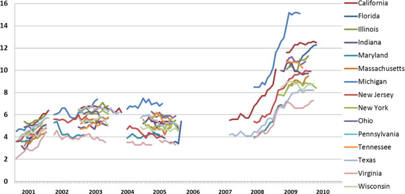
State Unemployment Rate (%) During Interview

Note: sample includes the 15 baseline states in FF

2.3. Control Variables

In models without maternal fixed-effects, we included a number of basic socioeconomic and demographic characteristics of the mother that were measured at baseline. These measures include dummy variables for mother’s age (<20, 20–23, 24–27, 28–32, 33+), race/ethnicity (white, black, Hispanic, and other race/ethnicity), education (less than high school, high school, some college, and college or more), immigrant status, marital/relationship status (married, cohabiting, and single), income (we use four categories of income-to-needs ratio¹⁸: poor is less than 1; near poor is income between 1 and less than 2; middle income is between 2 and less than 4; and high income is 4 or more), and child’s age (in months).

3. Methods

We estimate the effect of the UR on mother’s health using two logistic models, one that pools data from years 5 and 9 and controls for a rich set of covariates and year and state fixed-effects, and a second one that accounts for time-invariant mother fixed-effects. The following equation describes the first model:

$$Y_{\mathrm{i},\mathrm{t}}={\mathrm{\beta }}_0+{\mathrm{\beta }}_{1}U{R}_{\mathrm{i},\mathrm{t}}+{\mathrm{\beta }}_2{\mathbf{X}}_{\mathrm{i},\mathrm{t}-1}+{\alpha }_{\mathrm{s}}+{\alpha }_{\mathrm{t}}+{\epsilon }_{\mathrm{i},\mathrm{t}}$$ (1)

where Y_i,t denotes mother i’s health outcome measured at time t, UR is the average unemployment rate in baseline state s over the last year t from the date of interview, X is a matrix of mother characteristics measured at baseline (described above), and α_s and α_t are vectors of dummies for baseline state and year, respectively. The baseline state dummies control for any time-invariant state level factors that are correlated with both state economic conditions and women’s health. The year dummies will absorb year specific factors that could affect both the economy and mother’s health; ɛ is the disturbance term. All models are clustered at the baseline state level to account for within-state correlation in the observations. The coefficient of interest is β₁.

The second logistic model controls for mother-specific fixed-effects and is estimated using equation 2. The only covariate included in this model is α_t, the interview year dummy.

$$Y_{\mathrm{i},\mathrm{t}}={\mathrm{\beta }}_{\mathrm{i}}+{\mathrm{\beta }}_{1}U{R}_{\mathrm{i},\mathrm{t}}+{\alpha }_{\mathrm{t}}+{\epsilon }_{\mathrm{i},\mathrm{t}}$$ (2)

This model exploits the longitudinal nature of FF by including a mother-specific fixed effect, β_i, to control for observed and unobserved time-invariant characteristics of the mother, which may be correlated with both residing in a state with high UR and experiencing health problems. For instance, if a mother belongs to a demographic group that is likely to be particularly impacted by unemployment, she may also be more likely to suffer from health problems.

We estimate separate logistic fixed-effects models by subgroups. We stratify the sample by white, blacks, and Hispanics; marrieds versus unmarried women; and mothers with a high school degree or less versus those with more than a high school degree. We do these separate analyses because we expect to find heterogeneous impacts across groups, and in particular we hypothesize that the most disadvantaged women (minorities, unmarried, and the least educated) will fare worse during the Great Recession than more advantaged women, because they are less likely to be able to insure themselves against contingencies.

4. Results

4.1. Effects of the UR

Table 3 presents results from the pooled logistic and logistic fixed-effects models of the impacts of state unemployment rate on health and health behaviors. We only report the coefficient of interest, β₁, and when this coefficient is statistically significant at least at the 95 percent level of confidence, we show it in bold type. Under each individual estimate we report the percent change in the outcome that is associated with a one percentage point increase in the unemployment rate and we refer to these values to express the magnitude of the effects.

Table 3.

The Effect of the UR on Mother’s Health in FF

	Health status Excellent or Very Good	Health problem limits work	Obesity	Any health insurance	Smokes	>=4 Drinks on 1 Occasion	Drug use	Depressed
State UR
LOGIT	0.933	0.989	1.024	0.987	1.09	1.091	1.029	0.998
	[−1.755]	[−0.284]	[1.407]	[−0.334]	[1.810]	[1.852]	[0.471]	[−0.033]
% change in health outcome due to a 1pp increase in UR1	−2.9%	−0.9%	1.3%	−0.3%	5.6%	8.0%	2.9%	−0.2%
LOGIT-FE	0.848	1.073	1.087	0.993	1.256	1.140	1.400	0.941
	[−2.602]	[0.661]	[0.712]	[−0.111]	[2.231]	[1.521]	[2.499]	[−0.791]
% change	−4.3%	7.3%	2.4%	−0.1%	5.1%	6.9%	15.2%	−3.4%
City UR
LOGIT	0.916	1.058	1.025	0.956	1.088	1.062	1.128	0.994
	[−1.951]	[1.365]	[1.237]	[−0.971]	[1.790]	[1.339]	[1.576]	[−0.107]
% change	−3.8%	6.1%	1.6%	−0.9%	5.4%	4.1%	12.3%	−0.2%
LOGIT-FE	0.880	1.154	1.038	1.002	1.295	1.151	1.394	0.938
	[−2.112]	[1.451]	[0.332]	[0.030]	[2.650]	[1.640]	[2.738]	[−0.851]
% change	−4.2%	7.3%	1.9%	0.1%	4.5%	5.4%	9.8%	−4.4%
N	7,080	7,070	6,178	7,064	7,079	7,070	7,058	7,067
N changers	953	364	511	758	359	491	322	591

Note:

Each coefficient comes from a separate regression.

Logit models control for mother characteristics (age, race/ethnicity, education, income-to-needs ratio, and marital status), and baseline state (city) and year fixed-effects; errors are clustered at the baseline state (city) level (see equation 1). Logit-FE models control for year fixed-effects (see equation 2).

¹Predicted percent change in health outcome associated with a percentage point increase in the unemployment rate in year 9.

T-statistics are shown in brackets; bold font indicates that the result is statistically significant at the 95% level of confidence.

The logistic estimates (equation 1) shown in the first row, with one exception (depression), suggest that health gets worse as unemployment increases, but none of the coefficients are significantly different from zero at the 0.95 level of confidence. Self-reported health status and binge drinking are significant at the 0.90 level. While not shown in the regressions due to space limitations, a few covariates are significantly associated with health outcomes in the pooled logistic models. Women with high levels of education report better health outcomes than those with less than a high school degree. Single and cohabiting women have significantly worse health and health behaviors than those who are married. An increase in the income-to-needs ratio measured at baseline is significantly associated with an increase in health status as well as with an increase in substance use.

The second row of Table 3 shows models that control for individual fixed-effects. These estimates are remarkably similar in size to those obtained from the logistic models, but are more precisely estimated. The estimates confirm that as the economy worsens, women’s physical health declines and health compromising behaviors increase. During the recession, a one percentage point increase in the unemployment rate was associated with a decrease in the probability of experiencing “excellent” or “very good” physical health by 4.3 percent, and an increase in smoking or using drugs by 5.1 and 15.2 percent, respectively. These effects are larger than those of Davalos and French (2011) who focus on the 2001 recession (recession in which the UR went from 4.5. to 5.5%), and found that a 1 percentage point increase in the UR reduced overall physical health by 0.9%. It is possible that the larger effects are due to the much more massive scale of the recession.

No effects are observed on the probability of having health insurance. This result is consistent with Cawley, Moriya, and Simon (2011), who also find no effect on the probability of health insurance for both the working age population and for the sample of women with children.¹⁹ Table 3 also shows that the unemployment rate had no effect on obesity.²⁰ Previous studies have found mixed evidence on obesity (Charles and DeCicca, 2008; Ruhm, 2000, 2005), however, these studies have not examined the impacts of the UR on women. Moreover, no effects were observed on the probability of being depressed.²¹ Previous research has measured mental health with individual measures of self-rated feelings of sadness, hopelessness, or worthlessness, or with more extreme measures such as suicides. The CIDI-SF uses information about a list of different symptoms and their specific durations, and is used to determine a probable diagnosis of the psychiatric condition known as a major depressive episode. The fact that we do not observe an effect on this depression screener for the whole sample should not be seen as inconsistent with previous studies. For instance, a recent paper showed that while the 2008 stock market crash, which led to huge losses in wealth for many households, caused immediate declines in subjective measures of mental health, it did not increase validated measures of depressive symptoms or indicators of depression (McInerney et al., 2013). Moreover, this finding could reflect the fact that the effects of unemployment on mental health are not equally distributed across groups defined by gender, marital status, and education, a hypothesis we pursue further below.

The bottom panel of Table 3 shows estimates of the UR at the city level. Using the LAUS data, we construct a measure of the average unemployment rate in the mother’s original baseline city. We employ the city unemployment rate because it may be a more accurate representation of a woman’s own labor market opportunities. Results are highly consistent with those obtained using the state level UR. For example, a 1 percentage point increase in the city unemployment rate is associated with a 4.2% decrease in probability of having “excellent” or “very good” health (vs. a 4.3% decline when we use the state UR), a 4.5% increase in smoking (vs. 5.1%), and a 9.8% rise in drug use (vs. 15.1%). For this reason and because: i) the state unemployment rate may be more salient to a woman when she is forming her perception of economic conditions; ii) measurement error, selective migration, and selective attrition may be more likely to be problematic when focusing on local area (city) unemployment rates; and iii) most studies have employed the state unemployment rate to measure effects on health, in what follows we focus the discussion on results that use the state UR rather than the city UR.

4.2. Heterogeneous Effects

Table 3 presents the overall effects of the Great Recession. In what follows we examine differences by race/ethnicity, marital status, and education groups. We present only the logistic-fixed-effects models since these provide the more reliable estimates and under the coefficients of the unemployment rate, we show the corresponding percent changes in the outcome associated with a one percentage point increase in the UR. We provide a brief discussion of these results after presenting the findings.

Table 4 shows the effects of the UR for the whole sample of mothers, and by racial/ethnicity groups (white, black, and Hispanic), by marital status (married and unmarried), and by education levels (mothers with a high school degree or less, and those with more than a high school degree). The estimates reveal significant differences in the effects of UR on women’s health across subpopulations. In general more disadvantaged mothers – minorities, unmarried, and the less educated – were likely to suffer negative health impacts while more advantaged women actually experienced health improvements in certain dimensions.

Table 4.

Logit-FE Estimates of Effects of State UR by Groups Using FF

	Health status Excellent or Very Good	Health problem limits work	Obesity	Any health insurance	Smokes	>=4 Drinks on 1 Occasion	Drug use	Depressed
All	0.848	1.073	1.087	0.993	1.256	1.14	1.4	0.941
	[−2.602]	[0.661]	[0.712]	[−0.111]	[2.231]	[1.521]	[2.499]	[−0.791]
% change1	−4.3%	7.3%	2.4%	−0.1%	5.1%	6.9%	15.2%	−3.4%
White	0.909	0.939	0.508	1.034	1.512	1.594	1.23	0.663
	[−0.691]	[−0.252]	[−2.091]	[0.221]	[1.571]	[2.535]	[0.759]	[−2.402]
% change	−1.4%	−2.2%	−4.5%	1.2%	5.1%	4.7%	1.1%	−11.1%
Black	0.687	1.31	1.358	0.848	1.227	1.148	1.703	0.865
	[−3.009]	[1.532]	[1.312]	[−1.165]	[1.121]	[0.672]	[2.456]	[−1.002]
% change	−9.1%	11.9%	2.7%	−1.9%	3.6%	11.5%	10.1%	−8.0%
Hispanic	0.933	1.157	1.151	1.061	1.06	1.073	1.902	1.301
	[−0.781]	[0.792]	[0.850]	[0.651]	[0.341]	[0.564]	[1.602]	[1.982]
% change	−2.0%	9.0%	4.6%	2.2%	6.1%	0.8%	12.8%	18.2%
Married	1.054	0.663	0.761	1.064	0.903	1.079	1.656	0.596
	[0.342]	[−1.245]	[−0.993]	[0.334]	[−0.321]	[0.331]	[1.340]	[−2.371]
% change	0.1%	−7.0%	−1.4%	1.7%	−0.1%	5.3%	13.3%	−8.4%
Unmarried	0.811	1.146	1.197	0.964	1.31	1.128	1.292	1.018
	[−2.940]	[1.191]	[1.331]	[−0.520]	[2.462]	[1.291]	[1.732]	[0.211]
% change	−5.7%	9.9%	3.2%	−0.7%	5.6%	6.2%	11.8%	0.2%
More than HS	0.858	0.566	1.16	0.872	1.655	1.116	1.4	0.771
	[−1.301]	[−2.274]	[0.451]	[−1.147]	[2.119]	[0.742]	[1.291]	[−1.950]
% change	−4.0%	−6.6%	1.0%	−2.1%	11.8%	3.7%	12.2%	−3.8%
HS or less	0.856	1.364	1.127	1.047	1.144	1.162	1.413	1.062
	[−1.971]	[2.353]	[0.916]	[0.589]	[1.164]	[1.391]	[2.144]	[0.601]
% change	−4.5%	19.1%	4.9%	1.1%	2.9%	8.5%	14.8%	2.7%
N	7,080	7,070	6,178	7,064	7,079	7,070	7,058	7,067

Note:

Each coefficient comes from a separate regression.

Logit-FE models control for year fixed-effects (see equation 2).

¹Predicted percent change in health outcome associated with a percentage point increase in the unemployment rate in year 9.

T-statistics are shown in brackets; bold font indicates that the result is statistically significant at the 95% level of confidence.

Results by race/ethnicity indicate two patters that are: i) minorities faced more pronounced declines in their physical and mental health compared to whites and ii), whites experienced, at least in some respects, improvements in their health. As the unemployment rate increased, white women were less likely to be obese (the probability declined by 4.5%) and to report feelings of depression (the probability decreased by 11.1%). Whites were also 4.7% more likely to binge drink as the economy deteriorated.

The estimates for African-Americans (shown in the third row of Table 4) indicate that for each percentage point that the UR increased the probability of having “excellent” or “very good” health fell by 9.1% and that for using drugs rose by 10.1%. Hispanics also show a marginal increase in drug use and a significant deterioration in mental health (the probability of being depressed increased by 18.2%). This last result contradicts that found in Tekin et al., (2013), in which the Hispanic populations showed an improvement in mental health when state employment rate declined.

We now examine differences by marital status. We exploit the fact that the Fragile Families dataset oversamples births to unwed parents, and as a result, it is possible to study differences by mother’s relationship status (married versus unmarried), which is usually difficult to examine in other surveys. The findings indicate that unmarried mothers were hard hit by the Great Recession whereas it may have actually improved the mental health of married mothers. logistic fixed-effects estimates show that a percentage point rise in the UR was associated with a decrease in the probability of being depressed among married women (by 8.4%), whereas unmarried women were 5.7% less likely to have “excellent” or “very good” health and were more likely to adopt health compromising behaviors (the probability of smoking rose by a significant 5.6%.

Finally, results by education indicate that more educated women suffered less during the Great Recession as they were less likely to have problems that limited their work-related activities (the probability fell by 6.6% per one percentage point increase in unemployment) and were less likely to be depressed (a 3.8% reduction in this probability, although only significant at the 90% level of confidence). However, more educated women were also more likely to smoke (experiencing an 11.8% rise in their probability). Mothers with a high school degree or less on the other hand, faced a significant decline in their physical health as they were more likely to report “good”, “fair”, or “poor” health (4.5%) and more likely to have had problems that limited their work (the probability increased by 19.1%). In terms of health behaviors, less educated women faced a significant increase in drug use (14.8%).

The most surprising aspect of the results discussed above is that white, highly educated, and married women appear to suffer less from depression when the unemployment rate rises. A possible explanation is that groups with relatively low unemployment or risk of spousal unemployment feel themselves to be relatively better off in bad times. Of course these more advantaged women also drank and smoke more with high unemployment. It is possible that this finding reflects within group heterogeneity. For example, it could be that within the group of more educated mothers, a small minority of women increased their smoking and drinking enough to affect the group mean.

We compare the results shown in Table 4 to those in previous literature and we confirm that even differences across subgroups were larger during the Great Recession. For example, while we found that a 1 percentage point increase in the state UR reduced the probability of having “excellent” or “very good” health by 9.5% for African Americans, Davalos and French (2011) estimate a 1.2% reduction. Moreover, among more educated individuals our results show a non-significant 3.6% decline in physical health, while they find a 0.9% decrease.

5. Extensions

5.1. Heterogeneity in the timing of the Great Recession

In this section we ask whether the impacts of the Great Recession can be identified in the subsample of mothers who were interviewed for the last wave of the data after 2008, the year in which the Great Recession had already hit the economy. This group was definitely exposed to the crisis. This subsample includes 2,003 women (1,866 were interviewed in 2009 and 137 in 2010, representing 57% of the sample in year 9), of which 489 were married at their child’s birth. We estimate models 1 and 2 for this group of mothers and we find substantially similar effects of the UR on their health and health behaviors, although the effects are less precisely estimated than in the whole sample of women. Appendix Table 1 shows these results.

5.2. Heterogeneity in the sample of states

We now explore whether the impacts of the UR could be driven by certain states, for example, larger states such as California or Texas that together they represent 30% of the sample, or states that experienced the effects of the crisis more strongly such as Michigan or Ohio (i.e., the average unemployment rate for these two states, in the period of interest, is 7.5% while for the full sample is 5.9%). We found no evidence of this. Estimating our baseline regressions in different subsamples provides estimates that were consistent in size and direction to the effects shown in Table 3, but with relatively weaker power. These results are shown in Appendix Table 2.

5.3. Using discrete versus continuous health outcomes

Since logistic fixed-effects models are only identified by mothers who change their health status across waves, cases in which a mother experiences little change in her latent health condition (and for whom the change is not enough to generate a move from one “status” to another), are discarded. In this section we ask whether our results are robust to including these cases. We do this by investigating whether a mother’s body mass index– a more sensitive measure than obesity that captures both small and large changes in weight – could be affected by the unemployment rate. BMI increased substantially in the four years between the waves, from 27.1 to 29.2 (an increase of approx. 8%) while obesity increased from 27.9% to 37.1% (an increase of approx. 33%).²² Results are shown in Appendix Table 3 and they indicate that, although the UR is positively associated with changes in mother’s BMI, the coefficient is not statistically significant. This finding is consistent with the result we found on mother’s obesity – a positive but non-significant effect of the UR.

5.4. Other measures of economic fluctuations: Employment-to-Population Ratio

Unemployed workers who grow discouraged in their job search and do not actively participate in the labor market are not officially counted as unemployed. Hence, reductions in the unemployment rate may sometimes overstate improvements in the labor market. Alternatively, the unemployment rate may remain high even as employment is rising if discouraged workers come back to the labor market. Thus, in order to more adequately capture fluctuations in the labor market, we also investigate how the state employment-to-population ratio (ER) has affected women’s health. The ER is defined as the number of employed workers as a proportion of the total population aged 18–64 in a given state. We constructed an annual average ER measure using employment data from the LAUS that come from the Current Population Survey, and we appended it to FF data based on a mother’s baseline state of residence and her date of interview (see footnote 16).

Appendix Table 4 shows logistic fixed-effects estimates of the effects of the state employment-to-population ratio on health outcomes. We find consistent but weaker estimates compared to those obtained when using the state unemployment rate. That is, as the economy expands, women’s physical health tends to improve and substance use declines. We also find heterogeneous impacts across demographic groups, indicating that the positive effects of economic recovery (an increase in ER) are mostly experienced by minority, unmarried, and less educated mothers as they are more likely to have improvements in their physical and mental health as well as a decrease in the odds of using of drugs.

5.5. Association between the effects of UR and self-reported physical and mental health

A question that arises from using self-reported health measures is whether the effects of the UR on self-reported physical health could be driven by differences in perceived health that result from changes in mental health. In supplemental analyses (not shown here), we explored the sensitivity of the estimated effects of UR on physical health to including measures of a mother’s mental health as a control variable in the main specification (model 2). The estimates indicate that controlling for a mother’s depression in our main specification, does not significantly change the estimated coefficient on UR for other outcomes.

5.6. Selective migration

Less than 10% of sample mothers have migrated from the state in which they were first sampled at childbirth by year 9, so it seems unlikely that selective migration is driving our results. Moreover, when we ask how the unemployment rate affects the probability that a mother migrated to a different state, we find little overall effect. In order to investigate this issue, we constructed a dummy variable equal to one if a mother changed her state of residence from year 5 to year 9 and zero otherwise, and we regressed this indicator on the UR she experienced in year 5 controlling for her observable baseline characteristics, as well as on dummies for the baseline state and year fixed-effects. We did not find a significant overall relationship between unemployment in year 5 and having migrated between year 5 and year 9. We do, however, find some evidence of heterogeneity in the migration response to unemployment: mothers with some college education, immigrants, and those in better health at baseline are less likely to have migrated in response to changes in unemployment.

This result suggests that using unemployment in the baseline state introduces some measurement error, and that this measurement error is not entirely random. Random measurement error in the unemployment rate would tend to attenuate its estimated effect on ill health. If measured unemployment is systematically too large for the unhealthiest people (because they have moved to places with lower unemployment), then this will tend to overstate the effect of unemployment on ill health.

In order to investigate this possible bias, we estimate an alternative set of models using the unemployment rate in the actual state of residence in both waves. So for instance, if a mother who was originally (at baseline) sampled in Florida, moves to New York, between year 5 and year 9, then her UR measure will be the UR in Florida in year 5 and the UR in New York in year 9. In these models, there is no systematic measurement error in unemployment. However, since whether or not the mother moves between waves is a choice, these estimates may be biased instead by endogeneity. For example, if less healthy women are more likely to move, and if they move to lower unemployment states, then we would tend to under-estimate the relationship between unemployment and poor health in these models.

Appendix Table 6 shows logistic fixed-effects estimates of these alternative models using the unemployment in the mother’s actual state of residence in both waves. The estimates are very similar to those presented above, which suggests that our estimates are not greatly affected by selective migration.²³

5.7 Selective attrition

Another potential source of selection bias in this study is the presence of selective attrition from year 5 to year 9. Selective attrition may bias our estimates of UR on health outcomes if for instance, mothers who are interviewed in year 5 and not in year 9, are missing from the data perhaps due to experiencing material hardship in year 9 (e.g., telephone service disconnected), which could be correlated with an increase in the probability of experiencing poor health.

The attrition rate from year 5 to year 9 of FF is 19%.²⁴ To analyze whether the effect of UR on the probability of attrition was different for different groups, we perform a simple test in which we construct a dummy variable equal to one if a mother attrited from year 5 to year 9²⁵, and we regress this indicator on the UR she experienced in year 5, her observable characteristics interacted by the UR in year 5, and all other covariates as described in equation 1.²⁶ In the presence of selective attrition, the coefficients on the interaction between the UR and a woman’s characteristics should be statistically significant. We also examine selective attrition in terms of health outcomes (physical and mental health and health behaviors) by replicating the previous analysis on selective attrition based on women’s observable characteristics, but this time we interact a woman’s health outcomes in year 5 with the UR in year 5.

Appendix Tables 7 and 8 show estimates of selective attrition in terms of women’s observable characteristics and in terms of women’s health outcomes. We find little evidence of selective attrition in terms of mother characteristics. In fact, the only group that is less likely to attrite in year 9 are women with a college degree who faced high UR in year 5. In terms of health status in year 5 we also find little evidence of selective attrition. We do see, however, that women who suffer from obesity in year 5 are significantly more likely to attrite in year 9 after experiencing high unemployment. These findings suggest that selective attrition is not a big issue in our analysis. To the extent that there is selective attrition, women in better health (i.e., more educated, less likely to be obese, and less likely to consume drugs) are more likely to be interviewed in year 9, which may lead to an underestimate of the effect of the UR on women’s health.

6. Conclusions

This study contributes to the ongoing discussion of the relationship between economic fluctuations and people’s health, by providing new evidence of the effects of the Great Recession on a growing group of vulnerable families, unmarried women with children. Our results imply that increases in unemployment over the Great Recession period of 2007–2009, reduced the probability of having “excellent” or “very good” health and increased the probability of smoking and of using drugs. The effects are larger than those reported in the previous literature, for example, Davalos and French (2011) found that a one percentage point increase in the unemployment rate increased the probability of fair or poor health by 0.9% whereas we estimate an increase of 4.3%. These larger estimates are consistent with the fact that the Great Recession represented a massive and unprecedented economic shock for millions of families and so may have had larger effects than smaller previous recessions. We show that if we estimate models of the state UR on health outcomes without controlling for individual fixed-effects, the coefficients are very similar in magnitude to those obtained when we do account for these time-invariant characteristics, although they are less precisely estimated. Thus, in order to be able to identify more precise estimates of the UR, it is helpful to be able to follow individuals over time.

Previous studies have come to very different conclusions about the impacts of economic downturns on health. Most of this research, however, predates the Great Recession, and only a few studies have focused on the recent crisis. Most importantly, no study has yet focused on the groups who were most likely to be impacted by high unemployment rate (i.e., disadvantaged families) and this is particularly relevant considering the growing body of research showing that inequality starts in early life and that children of more disadvantaged mothers are more likely to be disadvantaged themselves.

We show that the Great Recession had heterogeneous effects on the health of women. While increases in unemployment worsened physical and mental health, and increased smoking and drug use among minorities, unmarried mothers, and less educated mothers more advantaged women may have actually experienced better mental health and some improvements in their physical health. For example, we found that whites were less likely to be obese and more educated women were less likely to have health problems during the Recession. However, the picture was mixed as they were also more likely to smoke and binge drink as the UR increased. These results are consistent with recent findings suggesting that the employment effects of the crisis were disproportionately concentrated in some subpopulations.

We faced several limitations. First, our sample is not generalizable to the population as a whole since FF is an urban birth cohort study; however, since the evidence in this area is limited, especially on women or disadvantaged groups, using FF contributes to the discussion. Second, all the measures that we have analyzed are self-reported and they have not been medically verified. Third, although we suggested potential pathways through which the recession could have affected women’s health, we did not directly test them.

Research that further explores the effect of economic conditions on the health outcomes of more disadvantaged groups should explore potential mechanisms driving these impacts. Many studies have argued that unemployment could impact people’s health through changes in health behavior or increasing stress due to income and wealth declines; however, whether the relative importance of these pathways differs across social groups and in particular for those experiencing a high economic burden remains an open question. Another useful extension of our work would be to investigate the impacts of the Recession on children’s health. The declines in mothers’ health, particularly among fragile families, could suggest important short and long-term effects on young children that could contribute to inequality for years to come.

Appendix Table 1.

The Effect of the UR on Mother’s Health for the Full sample and for the Sample Interviewed After 2008

	Health status Excellent or Very Good	Health problem limits work	Obesity	Any health insurance	Smokes	>=4 Drinks on 1 Occasion	Drug use	Depressed
Full sample
LOGIT	0.933	0.989	1.024	0.987	1.09	1.091	1.029	0.998
	[−1.755]	[−0.284]	[1.407]	[−0.334]	[1.810]	[1.852]	[0.471]	[−0.033]
LOGIT-FE	0.848	1.073	1.087	0.993	1.256	1.140	1.400	0.941
	[−2.602]	[0.661]	[0.712]	[−0.111]	[2.231]	[1.521]	[2.499]	[−0.791]
N	7,080	7,070	6,178	7,064	7,079	7,070	7,058	7,067
N changers	953	364	511	758	359	491	322	591
Sample interviewed AFTER 2008
LOGIT	0.929	0.99	1.018	0.966	1.089	1.046	1.048	0.978
	[−1.66]	[−0.182]	[0.712]	[−0.701]	[1.382]	[0.912]	[0.621]	[−0.283]
LOGIT-FE	0.842	1.013	1.017	1.025	1.214	1.188	1.252	0.935
	[−2.610]	[0.123]	[0.142]	[0.371]	[1.841]	[1.921]	[1.574]	[−0.832]
N	3,540	3,539	3,100	3,534	3,540	3,537	3,536	3,532
N changers	531	202	279	415	209	302	161	320

Note:

Each coefficient comes from a separate regression.

Logit models control for mother characteristics (age, race/ethnicity, education, income-to-needs ratio, and marital status), and baseline state and year fixed-effects; errors are clustered at the baseline state level (see equation 1). Logit-FE models control for year fixed-effects (see equation 2).

The sample interviewed after 2008 includes years 2009 and 2010.

T-statistics are shown in brackets; bold font indicates that the result is statistically significant at the 95% level of confidence.

Appendix Table 2.

The Effect of the UR on Mother’s Health for the Full sample and for Different Samples of States

	Health status Excellent or Very Good	Health problem limits work	Obesity	Any health insurance	Smokes	>=4 Drinks on 1 Occasion	Drug use	Depressed
Full sample
LOGIT	0.933	0.989	1.024	0.987	1.09	1.091	1.029	0.998
	[−1.755]	[−0.284]	[1.407]	[−0.334]	[1.810]	[1.852]	[0.471]	[−0.033]
LOGIT-FE	0.848	1.073	1.087	0.993	1.256	1.140	1.400	0.941
	[−2.602]	[0.661]	[0.712]	[−0.111]	[2.231]	[1.521]	[2.499]	[−0.791]
N	7,080	7,070	6,178	7,064	7,079	7,070	7,058	7,067
N changers	953	364	511	758	359	491	322	591
Excluding states with the highest population: CA and TX
LOGIT	0.906	1.002	1.017	0.955	1.120	0.99	1.018	0.911
	[−1.172]	[0.029]	[0.392]	[−0.731]	[1.372]	[−0.089]	[0.141]	[−1.001]
LOGIT-FE	0.768	0.987	1.093	0.971	1.275	1.198	1.459	0.859
	[−2.631]	[−0.087]	[0.512]	[−0.284]	[1.610]	[1.299]	[2.089]	[−1.288]
N	5,003	4,997	4,370	4,994	5,003	4,994	4,981	4,984
N changers	667	281	369	484	257	328	238	411
Excluding states with the highest avg. UR: MI and OH
LOGIT	0.906	0.988	1.029	0.986	1.095	1.119	1.015	1.038
	[−2.588]	[−0.299]	[1.413]	[−0.339]	[1.664]	[2.569]	[0.199]	[0.656]
LOGIT-FE	0.832	1.043	1.023	1.01	1.189	1.163	1.198	0.962
	[−2.819]	[0.369]	[0.189]	[0.149]	[1.639]	[1.709]	[1.277]	[−0.483]
N	6,375	6,367	5,567	6,360	6,375	6,365	6,346	6,363
N changers	859	315	447	696	324	441	279	523

Note:

Each coefficient comes from a separate regression.

Logit models control for mother characteristics (age, race/ethnicity, education, income-to-needs ratio, and marital status), and baseline state and year fixed-effects; errors are clustered at the baseline state level (see equation 1). Logit-FE models control for year fixed-effects (see equation 2).

T-statistics are shown in brackets; bold font indicates that the result is statistically significant at the 95% level of confidence.

Appendix Table 3.

The Effect of the State UR on Mother’s Weight

	Obesity		BMI
	Logit	OLS	OLS
State UR
Without individual FE	1.024	0.005	0.033
	[1.407]	[1.086]	[0.252]
With individual FE	1.087	0.009	0.056
	[0.712]	[1.164]	[0.727]
City UR
Without individual FE	1.025	0.006	0.042
	[1.237]	[1.261]	[0.341]
With individual FE	1.038	0.008	0.050
	[0.332]	[1.042]	[0.651]
N	6,178	6,178	6,178
N changers	511	511	2,541

Note:

Each coefficient comes from a separate regression.

Logit/OLS models control for mother characteristics (age, race/ethnicity, education, income-to-needs ratio, and marital status), and state (city) and year fixed-effects; errors are clustered at the baseline state (city) level (see equation 1). Logit-FE/Linear models with individual fixed-effects control for year fixed-effects (see equation 2).

T-statistics are shown in brackets; bold font indicates that the result is statistically significant at the 95% level of confidence.

Appendix Table 4.

Logit-FE Estimates of Effects of State ER Using FF

	Health status Excellent or Very Good	Health problem limits work	Obesity	Any health insurance	Smokes	>=4 Drinks on 1 Occasion	Drug use	Depressed
All	1.043	0.995	0.924	1.023	0.956	0.919	0.902	1.015
	[1.164]	[−0.09]	[−1.191]	[0.530]	[−0.774]	[−1.365]	[−1.576]	[0.341]
White	0.812	1.342	0.927	1.030	0.961	0.800	0.920	1.430
	[−1.700]	[1.708]	[−0.331]	[0.238]	[−0.265]	[−1.862]	[−0.531]	[2.611]
Black	1.006	0.967	0.975	1.081	0.983	1.022	0.873	1.021
	[0.142]	[−0.492]	[−0.312]	[1.396]	[−0.228]	[0.261]	[−1.676]	[0.352]
Hispanic	1.043	0.995	0.821	0.835	1.044	0.878	1.009	0.706
	[1.155]	[−0.094]	[−1.142]	[−1.844]	[0.249]	[−1.075]	[0.031]	[−2.764]
Married	0.932	1.045	0.783	0.877	1.075	0.843	–	1.278
	[−0.857]	[0.337]	[−1.292]	[−1.183]	[−0.421]	[−1.261]		[2.004]
Unmarried	1.070	0.990	0.940	1.062	0.930	0.961	0.874	0.981
	[1.643]	[−0.165]	[−0.863]	[1.281]	[−1.132]	[−0.660]	[−1.772]	[−0.381]
More than HS	0.963	1.284	1.006	0.999	0.995	0.891	0.966	1.291
	[−0.588]	[2.279]	[0.043]	[−0.013]	[−0.04]	[−1.190]	[0.281]	[2.742]
HS or less	1.080	0.899	0.895	1.031	0.941	0.953	0.871	0.934
	[1.714]	[−1.599]	[−1.439]	[0.621]	[−0.904]	[−0.718]	[0.070]	[−1.241]
N	7,080	7,070	6,178	7,064	7,079	7,070	7,058	7,067

Note:

Each coefficient comes from a separate regression.

Logit-FE models include year fixed-effects (see equation 2).

T-statistics are shown in brackets; bold font indicates that the result is statistically significant at the 95% level of confidence.

Appendix Table 5.

Logit-FE Estimates of Effects of UR controlling for a Mother’s Current State of Residence

	Health status Excellent or Very Good	Health problem limits work	Obesity	Any health insurance	Smokes	>=4 Drinks on 1 Occasion	Drug use	Depressed
WITHOUT current state of residence controls	0.848	1.073	1.087	0.993	1.256	1.140	1.400	0.941
	[−2.602]	[0.661]	[0.712]	[−0.111]	[2.231]	[1.521]	[2.499]	[−0.791]
WITH current state of residence controls	0.839	1.086	1.112	1.022	1.320	1.135	1.427	0.967
	[−2.770]	[0.781]	[0.884]	[0.33]	[2.672]	[1.483]	[2.603]	[−0.43]
N	7,080	7,070	6,178	7,064	7,079	7,070	7,058	7,067
N changers	953	364	511	758	359	491	322	591

Note:

Each coefficient comes from a separate regression.

All models (Logit-FE models) include year fixed-effects (see equation 2); in addition to year fixed-effects, models in the 3^rd row (“WITH current state of residence controls”) include current state fixed-effects.

T-statistics are shown in brackets; bold font indicates that the result is statistically significant at the 95% level of confidence.

Appendix Table 6.

Logit-FE Estimates of Effects of Current State of Residence UR in Using FF

	Health status Excellent or Very Good	Health problem limits work	Obesity	Any health insurance	Smokes	>=4 Drinks on 1 Occasion	Drug use	Depressed
All	0.853	1.091	1.073	0.992	1.220	1.108	1.355	1.019
	[−2.644]	[0.827]	[0.632]	[−0.125]	[2.046]	[1.251]	[2.509]	[0.258]
White	0.931	1.086	0.824	1.008	1.459	1.216	1.232	0.767
	[−0.442]	[0.328]	[−0.722]	[0.052]	[1.616]	[1.152]	[0.899]	[−1.593]
Black	0.706	1.321	1.175	0.933	1.149	1.276	1.480	0.955
	[−3.138]	[1.644]	[0.772]	[−0.558]	[0.832]	[1.338]	[2.134]	[−0.372]
Hispanic	0.925	1.067	1.072	1.046	1.076	1.058	1.942	1.339
	[−0.915]	[0.359]	[0.434]	[0.495]	[0.423]	[0.455]	[1.669]	[2.170]
Married	1.080	0.588	0.782	0.983	1.019	0.951	1.734	0.715
	[0.547]	[−1.622]	[−1.030]	[−0.097]	[0.060]	[−0.220]	[1.630]	[−1.700]
Unmarried	0.807	1.205	1.186	0.968	1.278	1.120	1.225	1.095
	[−3.146]	[1.609]	[1.299]	[−0.477]	[2.327]	[1.279]	[1.508]	[1.106]
More than HS	0.882	0.599	1.347	0.924	1.359	1.104	1.441	0.881
	[−1.151]	[−2.091]	[1.009]	[−0.738]	[1.461]	[0.677]	[1.563]	[−1.016]
HS or less	0.850	1.319	1.088	1.026	1.155	1.120	1.341	1.122
	[−2.222]	[2.160]	[0.673]	[0.334]	[1.297]	[1.100]	[1.991]	[1.195]
N	7,080	7,070	6,178	7,064	7,079	7,070	7,058	7,067

Note:

Each coefficient comes from a separate regression.

Logit-FE models include year fixed-effects (see equation 2).

T-statistics are shown in brackets; bold font indicates that the result is statistically significant at the 95% level of confidence.

Appendix Table 7.

The Propensity to Attrite in Year 9 Explained by the UR in Year 5 and Women’s Characteristics

	(1)	(2)
UR	1.711	5.291
	[2.061]	[1.001]
UR * Mother’s Age <20		1.001
		[0.006]
UR * Mother’s Age 20–23		0.979
		[−0.208]
UR * Mother’s Age 24–27		0.991
		[−0.118]
UR * Mother’s Age 28–32		1.001
		[0.021]
UR * Mother is Black		0.821
		[−1.187]
UR * Mother is Hispanic		0.774
		[−1.129]
UR * Mother is other race/ethn		0.787
		[−1.693]
UR * Mother is immigrant		1.062
		[0.338]
UR * Mother is single		0.814
		[−1.015]
UR * Mother cohabitates		0.894
		[−0.616]
UR * Mother’s Educ HS		0.905
		[−0.992]
UR * Mother’s Educ Some College		0.819
		[−3.733]
UR * Mother’s Educ College		0.759
		[−1.131]
UR * Mother’s income-to-needs ratio <100%		1.014
		[0.150]
UR * Mother’s inc.-to-needs ratio: 100–199%		1.099
		[0.718]
UR * Mother’s inc.-to-needs ratio: 200–399%		1.111
		[0.662]
UR * Child’s Age in months		0.988
		[−0.510]
N	3,797	3,797

Note:

Each column is a separate regression. Sample includes year 9 data as a cross section. The state UR is measured in year 5. In addition to the listed covariates, both regressions include main effects for mother’s age, race/ethnicity, education, income-to-needs ratio, and marital status as well as baseline state and year fixed-effects; errors are clustered at the baseline state level.

T-statistics are shown in brackets; bold font indicates that the result is statistically significant at the 95% level of confidence.

Appendix Table 8.

The Propensity to Attrite in Year 9 Explained by UR and Mother’s Health in Year 5

	(1)	(2)
UR	1.727	1.747
	[1.754]	[1.765]
UR * Health is Excellent or V. good		0.989
		[−0.122]
UR * Health problem limits work		0.749
		[−1.605]
UR * Obesity		1.321
		[4.201]
UR * Any health insurance		0.882
		[−1.920]
UR * Smokes		1.088
		[1.036]
UR * 4>= Drinks in 1 Occasion		0.916
		[−0.740]
UR * Uses drugs		1.207
		[1.777]
UR * Depressed		1.016
		[0.114]
N	3,472	3,472

Note:

Each column is a separate regression. The state UR and all health variables (health status, health problem that limits work, obesity, etc.) are measured in year 5. In addition to the listed covariates, both regressions include main effects for mother’s age, race/ethnicity, education, income-to-needs ratio, and marital status as well as baseline state and year fixed-effects; errors are clustered at the baseline state level.

T-statistics are shown in brackets; bold font indicates that the result is statistically significant at the 95% level of confidence.

References

- Aalto-Setälä T, Haarasilta L, Marttunen M, Tuulio-Henriksson A, Poikolainen K, Aro H, Lönnqvist J. Major Depressive Episode among Young Adults: CIDI-SF versus Scan Consensus Diagnosis. Psychological Medicine. 2002;32:1309–1314. doi: 10.1017/s0033291702005810. [DOI] [PubMed] [Google Scholar]
- Acs G, Nelson S. The Kids are Alright? Children’s Well-Being and the Rise of Cohabitation. Washington D.C.: The Urban Institute; 2002. [Google Scholar]
- Almond D, Currie J. Human Capital Development before Age Five. In: Card D, Ashenfelter O, editors. Handbook of Labor Economics. part B. Vol. 4. New York: American Elsevier Publishing Co; 2011. pp. 1315–1486. chapter 15. [Google Scholar]
- American Psychiatric Association. Diagnostic and Statistical Manual of Mental Disorders. 4th. Washington D.C.: American Psychiatric Association; 1994. [Google Scholar]
- Artazcoz L, Benach J, Borrell C, Cortès I. Unemployment and Mental Health: Understanding the Interactions among Gender, Family Roles, and Social Class. American Journal of Public Health. 2004;94(1):82–88. doi: 10.2105/ajph.94.1.82. [DOI] [PMC free article] [PubMed] [Google Scholar]
- Ásgeirsdóttir TL, Corman H, Noonan K, Ólafsdóttir Þ, Reichman NE. NBER. 2012. Are Recessions Good for Your Health Behaviors? Impacts of The economic Crisis in Iceland; p. 18233. (Working Paper). [Google Scholar]
- Becker G. A Treatise on the Family. Cambridge: Harvard University Press; 1981. [Google Scholar]
- Browning M, Heinesen E. Effect of Job Loss Due to Plant Closure on Mortality and Hospitalization. Journal of Health Economics. 2012;31(4):599–616. doi: 10.1016/j.jhealeco.2012.03.001. [DOI] [PubMed] [Google Scholar]
- Bureau of Labor Statistics. News Release: The Employment Situation June, 2013. 2013 Jul; http://www.bls.gov/news.release/pdf/empsit.pdf.
- Case A, Fertig A, Paxson C. The Lasting Impact of Childhood Health and Circumstance. Journal of Health Economics. 2005;24(2):365–389. doi: 10.1016/j.jhealeco.2004.09.008. [DOI] [PubMed] [Google Scholar]
- Cawley J, Moriya AS, Simon KI. NBER. 2011. The Impact of the Macro-economy on Health Insurance Coverage: Evidence from the Great Recession; p. 17600. (Working Paper). [Google Scholar]
- Charles KK, DeCicca P. Local labor Market Fluctuations and Health: Is There a Connection and for Whom? Journal of Health Economics. 2008;27(6):1532–1550. doi: 10.1016/j.jhealeco.2008.06.004. [DOI] [PubMed] [Google Scholar]
- Center for Budget Policy and Priorities. Chart Book: The Legacy of the Great Recession. Special Series: Economic Recovery Watch. 2013 Jul; http://www.cbpp.org/cms/index.cfm?fa=view&id=3252.
- Center for Disease Control and Prevention. Summary Health Statistics for U.S. Adults. (series 10).National Health Interview Survey, 2011- Vital and Health Statistics. 2012 Dec;(256) http://www.cdc.gov/nchs/data/series/sr_10/sr10_256.pdf. [PubMed]
- Center for Disease Control and Prevention. Mental Health among Women of Reproductive Age. Division of Reproductive Health. 2013 http://www.cdc.gov/reproductivehealth/Depression/PDFs/Mental_Health_Women_Repo_Age.pdf.
- Currie J. Healthy, Wealthy, and Wise? Socioeconomic Status, Poor Health in Childhood, and Human Capital Development. Journal of Economic Literature. 2009;47(1):87–122. [Google Scholar]
- Currie J, Madrian B. Health, Health Insurance and the Labor Market. In: Card D, Ashenfelter O, editors. The Handbook of Labor Economics. 3c. Amsterdam: North Holland; 1999. pp. 3309–3407. [Google Scholar]
- Currie J, Stabile M. Socioeconomic Status and Child Health: Why Is the Relationship Stronger for Older Children? American Economic Review. 2003;93(5):1813–1823. doi: 10.1257/000282803322655563. [DOI] [PubMed] [Google Scholar]
- Davalos ME, French MT. This Recession Is Wearing Me Out! Health-Related Quality of Life and Economic Downturns. Journal of Mental Health and Economic Policy. 2011;14(2):61–72. [PubMed] [Google Scholar]
- Davalos ME, Fang H, French MT. Easing the Pain of an Economic Downturn: Macroeconomic Conditions and Excessive Alcohol Consumption. Health Economics. 2012;21(11):1318–1335. doi: 10.1002/hec.1788. [DOI] [PMC free article] [PubMed] [Google Scholar]
- Dee TS. Alcohol Abuse and Economic Conditions: Evidence from Repeated Cross-Sections of Individual-Level Data. Health Economics. 2001;10(3):257–270. doi: 10.1002/hec.588. [DOI] [PubMed] [Google Scholar]
- Deb P, Gallo WT, Ayyagari P, Fletcher J, Sindelar J. The Effect of Job Loss on Overweight and Drinking. Journal of Health Economics. 2011;30(2):317–327. doi: 10.1016/j.jhealeco.2010.12.009. [DOI] [PMC free article] [PubMed] [Google Scholar]
- Dehejia R, Lleras-Muney A. Booms, Busts, and Babies’ Health. Quarterly Journal of Economics. 2004;119(3):1091–1130. [Google Scholar]
- DiMatteo MR, Giordani PJ, Lepper HS, Croghan TW. Patient Adherence and Medical Treatment Outcomes: A Meta-Analysis. Med Care. 2002;40(9):794–811. doi: 10.1097/00005650-200209000-00009. [DOI] [PubMed] [Google Scholar]
- Eliason M, Storrie D. Does Job Loss Shorten Life? Journal of Human Resources. 2009a;44(2):277–302. [Google Scholar]
- Eliason M, Storrie D. Job Loss is Bad for Your Health: Swedish Evidence on Cause-Specific Hospitalization Following Involuntary Job Loss. Social Science and Medicine. 2009b;68(8):1396–1406. doi: 10.1016/j.socscimed.2009.01.021. [DOI] [PubMed] [Google Scholar]
- Fischer JA, Sousa-Poza A. Does Job Satisfaction Improve the Health of Workers? New Evidence Using Panel Data and Objective Measures of Health. Health Economics. 2009;18(1):71–89. doi: 10.1002/hec.1341. [DOI] [PubMed] [Google Scholar]
- Gerdtham UG, Ruhm C. Deaths Rise in Good Economic Times: Evidence from the OECD. Economics & Human Biology. 2006;4(3):298–316. doi: 10.1016/j.ehb.2006.04.001. [DOI] [PubMed] [Google Scholar]
- Geronimus AT. The Weathering Hypothesis and the Health of African-American Women and Infants: Evidence and Speculations. Ethn Dis. 1992;2(3):207–221. [PubMed] [Google Scholar]
- Grossman M. The Demand for Health: A Theoretical and Empirical Investigation. New York: National Bureau of Economic Research; 1972. [Google Scholar]
- Grusky D, Western B, Wimer C. In: The Great Recession. Grusky D, Western B, Wimer C, editors. New York: Russell Sage Foundation; 2011. [Google Scholar]
- Hoynes HW, Miller D, Schaller J. Who Suffers During Recessions? Journal of Economic Perspectives. 2012;26(3):27–48. [Google Scholar]
- Huff-Stevens A, Miller DL, Page ME, Filipski M. NBER. 2011. The Best of Times, the Worst of Times: Understanding Pro-cyclical Mortality; p. 17657. (Working Paper). [DOI] [PMC free article] [PubMed] [Google Scholar]
- Katz SJ, Hofer TP. Socioeconomic Disparities in Preventive Care Persist Despite Universal Coverage: Breast and Cervical Cancer Screening in Ontario and the United States. JAMA. 1994;272(7):530–534. [PubMed] [Google Scholar]
- Kessler R, Mroczek D. Final Version of our Non-specific Psychological Distress Scale. Ann Arbor, MI: Survey Research Center of the Institute for Social Research, University of Michigan; 1994. [Google Scholar]
- Kessler R, Andrews G, Mroczek D, Ustun B, Wittchen HU. The World Health Organization Composite International Diagnostic Interview Short-Form (CIDI-SF) International Journal of Methods in Psychiatric Research. 1998;7(4):171–185. [Google Scholar]
- Kim MH, Kim C, Park JK, Kawachi I. Is Precarious Employment Damaging to Self-Rated Health? Social Science & Medicine. 2008;67(12):1982–94. doi: 10.1016/j.socscimed.2008.09.051. [DOI] [PubMed] [Google Scholar]
- Kliesen KL. The 2001 Recession: How Was It Different and What Developments May Have Caused It? Federal Reserve Bank of St Louis, Economic Research. 2003 Sep-Oct;85(5):23–38. 2003. http://research.stlouisfed.org/publications/review/03/09/Kliesen.pdf. [Google Scholar]
- Kochhar R. Pew Research Social and Demographic Trends Project. Pew Research Center; Washington DC: 2011. Two Years of Economic Recovery: Women Lose Jobs, Men Find Them. http://www.pewsocialtrends.org/2011/07/06/two-years-of-economic-recovery-women-lose-jobs-men-find-them/ [Google Scholar]
- Kochhar R, Richard F, Taylor T. Pew Research Social and Demographic Trends Project. Pew Research Center; Washington DC: 2011. Wealth Gaps Rise to Record Highs Between Whites, Blacks, and Hispanics. [Google Scholar]
- Lam D. Marriage Markets and Assortative Mating with Household Public Goods: Theoretical Results and Empirical Implications. Journal of Human Resources. 1988;23(4):462–487. [Google Scholar]
- Mani A, Mullainathan S, Shafir E, Zhao J. Poverty Impedes Cognitive function. Science. 2013;341:976–980. doi: 10.1126/science.1238041. [DOI] [PubMed] [Google Scholar]
- McClure CB, Valdimarsdóttir UA, Hauksdóttir A, Kawachi I. Economic Crisis and Smoking Behaviour: Prospective Cohort Study in Iceland. BMJ. 2013;2(5):1–7. doi: 10.1136/bmjopen-2012-001386. [DOI] [PMC free article] [PubMed] [Google Scholar]
- McInerney M, Mellor JM, Nicholas LH. Recession Depression: Mental Health Effects of the 2008 Stock Market Crash. Journal of Health Economics. 2013;32(6):1090–1104. doi: 10.1016/j.jhealeco.2013.09.002. [DOI] [PMC free article] [PubMed] [Google Scholar]
- Miilunpalo S, Vuori I, Oja P, Pasanen M, Urponen H. Self-rated Health Status as a Health Measure: The Predictive Value of Self-reported Health status on the Use of Physician Services and on Mortality in the Working-age Population. J Clin Epidemiol. 1997;50(5):517–28. doi: 10.1016/s0895-4356(97)00045-0. [DOI] [PubMed] [Google Scholar]
- Murphy GC, Athanasou JA. Unemployment and General Health: A Review and Evaluation. Journal of Occupational and Organisational Psychology. 1999;72:83–99. [Google Scholar]
- Neumayer E. Recessions Lower (some) Mortality Rates: Evidence from Germany. Social Science & Medicine. 2004;58(6):1037–1047. doi: 10.1016/s0277-9536(03)00276-4. [DOI] [PubMed] [Google Scholar]
- Pfeffer TF, Danziger S, Schoeni RF. Wealth Disparities Before and After the Great Recession. The ANNALS of the American Academy of Political and Social Science. 2013;650:98–123. doi: 10.1177/0002716213497452. [DOI] [PMC free article] [PubMed] [Google Scholar]
- Reichman N, Teitler J, Garfinkel I, McLanahan S. Fragile Families: Sample and Design. Children and Youth Services Review. 2001;23(4/5):303–326. [Google Scholar]
- Ross CE, Van Willigen M. Gender, Parenthood, and Anger. Journal of Marriage and Family. 1996;58(3):572–584. [Google Scholar]
- Ruhm C. The Extent and Consequences of High School Employment. Journal of Labor Research. 1995;16(3):293–304. [Google Scholar]
- Ruhm C. Are Recessions Good for Your Health? Quarterly Journal of Economics. 2000;115(2):617–650. [Google Scholar]
- Ruhm C. Good Times Make You Sick. Journal of Health Economics. 2003;22(4):637–658. doi: 10.1016/S0167-6296(03)00041-9. [DOI] [PubMed] [Google Scholar]
- Ruhm C. Healthy Living in Hard Times. Journal of Health Economics. 2005;24(2):341–363. doi: 10.1016/j.jhealeco.2004.09.007. [DOI] [PubMed] [Google Scholar]
- Ruhm C, Black WE. Does Drinking Really Decrease in Bad Times? Journal of Health Economics. 2002;21(4):659–678. doi: 10.1016/s0167-6296(02)00033-4. [DOI] [PubMed] [Google Scholar]
- Sierminska E, Takhtamanova Y. Job Flows, Demographics, and the Great Recession. In: Immervoll P, Tatsiramos K, editors. Who Loses in the Downturn? Economic Crisis, Employment, and Income Distribution. Vol. 32. Emerald Group Publishing Limited; 2011. pp. 115–154. (Books Series: Research in Labor Economics). [Google Scholar]
- Sullivan D, von Wachter T. Job Displacement and Mortality: An Analysis using Administrative Data. Quarterly Journal of Economics. 2009;124(3):1265–1306. [Google Scholar]
- Tekin E, McClellan C, Minyard KJ. Health and Health behaviors During the Worst of Times: Evidence from the Great Recession. (Working Paper).NBER. 2013:19234. [Google Scholar]
- Theodossiou I. The Effects of Low-Pay and Unemployment on Psychological Well-Being: A Logistic Regression Approach. Journal of Health Economics. 1997;17(1):85–104. doi: 10.1016/s0167-6296(97)00018-0. [DOI] [PubMed] [Google Scholar]
- Turner JB. Economic Context and the Health Effects of Unemployment. Journal of Health and Social Behavior. 1995;36(3):213–229. [PubMed] [Google Scholar]
- Verick S. Who Is Hit Hardest during a Financial Crisis? The Vulnerability of Young Men and Women to Unemployment in an Economic Downturn. In: Islam I, Verick S, editors. From the Great Recession to Labour Market Recovery: Issues, Evidence and Policy Options. Basingstoke, Hampshire, UK: 2010. [Google Scholar]
- Xu X, Kaestner R. The Business Cycle and Health Behaviors. (Working Paper).NBER. 2010:15737. [Google Scholar]
Associated Data
This section collects any data citations, data availability statements, or supplementary materials included in this article.