Robust w-Estimators for Cryo-EM Class Means

Abstract

A critical step in cryogenic electron microscopy (cryo-EM) image analysis is to calculate the average of all images aligned to a projection direction. This average, called the “class mean”, improves the signal-to-noise ratio in single particle reconstruction (SPR). The averaging step is often compromised because of outlier images of ice, contaminants, and particle fragments. Outlier detection and rejection in the majority of current cryo-EM methods is done using cross-correlation with a manually determined threshold. Empirical assessment shows that the performance of these methods is very sensitive to the threshold. This paper proposes an alternative: a “w-estimator” of the average image, which is robust to outliers and which does not use a threshold. Various properties of the estimator, such as consistency and influence function are investigated. An extension of the estimator to images with different contrast transfer functions (CTFs) is also provided. Experiments with simulated and real cryo-EM images show that the proposed estimator performs quite well in the presence of outliers.

I. Introduction

Cryogenic electron microscopy (cryo-EM) is a relatively new imaging technique that aims to reconstruct the three-dimensional (3D) structure of biological macromolecules (e.g. protein molecules), called particles, from their two-dimensional (2D) projection images [2]. Cryo-EM does not require crystallization and the particles are maintained in their native hydrated state. These advantages, however, come at a cost: cryo-EM images are extremely noisy with signal-to-noise ratios (SNR) commonly below 0dB. The SNR is improved by averaging images that are believed to be from the same projection direction. The resulting average images are called class means.

In practice, many of the images that participate in the averaging turn out to be outliers. They arise from structures that are unrelated to the molecule (e.g., ice, contaminants) [3]. The presence of outliers at the averaging step compromises the fidelity of the reconstruction. Detecting such outlier images is a key problem in cryo-EM reconstruction [4].

Current outlier detection strategies in cryo-EM are mostly based on cross-correlating the images with one or more templates [5], [6]. Images with cross-correlation below a threshold are regarded as outliers. This approach is found in popular cryo-EM packages such as EMAN, SPIDER, Bsoft and SIGNATURE [7]–[10]. This classical approach has a serious drawback: its performance is sensitive to the threshold. The useful range of the threshold is narrow, difficult to find, and dependent on the image SNR. The false negative rate and the false positive rate increase rapidly as the threshold deviates from the optimal range [11]. Quite often the threshold has to be manually adjusted to the SNR of the image [7], [12], [13]. Manual adjustment is also problematic because outliers are often not visible to naked eye due to the low SNR.

In this paper, we propose an alternative approach that does not rely on thresholding. Drawing on classical robust estimation theory, we present a “w-estimator” for class means that is robust to outliers. The estimator is based on an outlier model specific to cryo-EM. Theoretical analysis shows that the influence function of the estimator is bounded for typical cryo-EM outliers. The reader should be aware that the analysis of the influence function is rather complex. One part of the analysis is in closed form, while one part is numerical. The numerical part is generic in the sense that it can be applied to any class mean, and is not restricted to a specific example. We also show that the estimator is Fisher-consistent.

A few methods in cryo-EM literature use w-estimator-like techniques, e.g., FREALIGN calculates the 3D reconstruction by a weighted sum of all images [14]. A similarity measure in the form of weighted frequency components is proposed to align cryo-EM images [15]. To our knowledge, these estimators are not explicitly derived in a w-estimator robust estimation theory framework. Their outlier model is not explicit, and theoretical properties such as consistency and robustness are not addressed. The parameters used in these algorithms are also set in an ad-hoc manner.

Common-lines based outlier detection methods correlate images with particle images from all projection directions on the common-lines [16]. Although such a method incorporates more images than the classical approach, it has similar drawbacks resulting from using thresholds for outlier rejection.

Approaches not based on thresholds are also possible. By classifying cryo-EM images into heterogeneous classes (e.g. using RELION [17]) and analyzing the reconstructed classes, classes that are visually inconsistent with the known structures of the molecule components are rejected as outliers [18], [19].

Extensive simulations are provided to compare the performances of the w-estimator and conventional outlier detection. Additionally, experiments with real cryo-EM data are also reported. They show that the w-estimator can suppress outliers in real-world cases.

Cryo-EM images are affected by the microscope contrast transfer function (CTF). To provide some insensitivity to the CTF, the particle is often imaged at different CTFs. We extend the w-estimator to this case, so that the class mean can be calculated from images acquired at different CTFs. Fisher-consistency and boundedness of the influence function for outliers also hold for this estimator.

The rest of the paper is organized as follows. Section II contains background information on cryo-EM. This section is included for readers who may be unfamiliar with cryo-EM and is also meant for fixing terminology and for stating the two problems we address. Section III contains the proposed estimator for the single CTF case and provides theoretical analysis of the estimator. Section IV extends the estimator to multiple CTFs. Section V shows the results of using the proposed w-estimators with simulated and real cryo-EM data. Section VI concludes the paper. Proofs of all claims are available in the Appendix.

II. The Cryo-EM Class Mean Problem

A. Cryo-EM and Reconstruction

In cryo-EM, projection images, called micrographs containing copies of the same particle embedded in vitreous ice are obtained. Sub-images of individual particles, referred to as particle images, are extracted from the micrograph using a template. Imperfections in the micrograph are caused by incompletely formed or disassembled particles due to sample preparation and contaminants. These “non-particles” are often mistakenly selected as particle images.

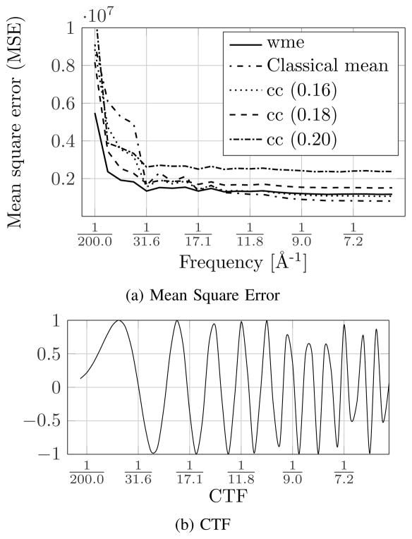
The formation of a cryo-EM image can be modeled as a tomographic projection of the particle from a random direction, convolved with a filter, followed by additive noise [2]. The kernel of filter is called the contrast transfer function (CTF). CTF arises from the interaction of the electron beam, the molecule, and the ice. Theoretical analysis suggests that CTF has a Fourier transform that is real, circularly symmetric, and taking positive and negative values (Fig. 9b). The CTF (the zeros of the CTF) can be changed using the defocus setting of the microscope.

Fig. 9.

Mean square error (MSE) of the w-estimator (wme), classical mean and cross-correlation (cc) with different thresholds for outlier rejection. 0.18 is the optimal threshold for cc. 45% outliers and SNR of −16dB. (a) shows the MSEs at different frequencies. (b) is the CTF of the images.

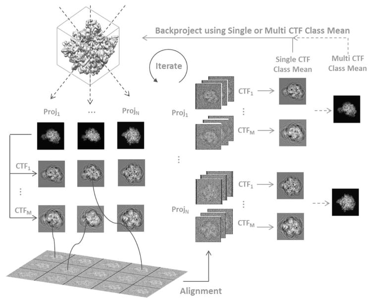
Particle images are used in an iterative procedure to reconstruct the 3D structure of the particle. Fig. 1 illustrates the reconstruction process using class means. There are reconstruction methods such as FREALIGN [14], that do not use class means for reconstruction (nevertheless, even for these methods the calculation of a class mean can be used for outlier detection, as this paper shows). Starting from an initial estimate of the structure, projections are obtained from many fixed directions and CTFs are applied to each projection. After allowing for in-plane rotation and translation, every particle image is associated with the most similar CTF-filtered projection, and the aligned images are averaged to give a class mean. Correlation or its variants are often used as similarity measure for alignment [20], [21]. The class means are backprojected to obtain a new estimate of the structure for the next iteration. An alternative reconstruction strategy is also possible: For every projection direction, the class means at different CTFs can be combined into a CTF-corrected class mean which is then backprojected to give the reconstruction.

Fig. 1.

Outline of reconstruction procedure.

Ideally, only particle images which come from a projection direction are aligned to that direction. In reality, some non-particle images plus some particle images from neighboring projection directions are also aligned (misaligned images). We refer to these images as outliers and the proposed method deals with these outlier images.

B. The Two Class Mean Estimation Problems

We can now state the two problems that we address in this paper:

1. Single CTF Class Mean: Given a set of images aligned to a single CTF at a projection direction, estimate the class mean robustly in the presence of outliers.

2. Multi CTF Class Mean: Given a set of images aligned to more than one CTF at a projection direction, estimate the CTF-corrected class mean robustly in the presence of outliers.

C. The Outlier Model

To proceed, we need a mathematical model for outliers. Recall that outliers are images of non-particles and misaligned particles and that outliers are detected according to their correlation coefficients with a reference during both particle extraction and alignment. Under this condition, the signal in the outlier has a low, but non-zero correlation coefficient with the matching template. The outlier model used below is based on this observation.

We also assume that the image noise is white. Although cryo-EM images do not follow this assumption exactly, pre-whitening filters are often designed and used [22].

III. Class Mean Estimation for Single CTF

A. Image Model

Suppose that x ∈ ℝ^p is a noisy image of p pixels obtained at a CTF, and aligned to a projection direction:

$$\mathbf{x}={\mathit{\theta }}_x+\mathbf{n},$$ (1)

where n is zero-mean Gaussian white noise with covariance matrix σ²I, and θ_x ∈ ℝ^p is the deterministic but unknown signal in the image. The expression for θ_x depends on whether the image is an inlier or an outlier:

Inlier

When the image x is an inlier

$${\mathit{\theta }}_x=s\mathit{\theta },$$ (2)

where θ(||θ|| > 0) is the non-noisy projection of the particle. θ incorporates the effect of CTF (and possibly the pre-whitening filter). The amplitude factor s is assumed to have a uniform probability density π(s|a, b) in an interval (a, b) which is symmetric about 1. This models real-world change in signal amplitude [23]. The probability density function (pdf) of x is obtained by marginalizing s:

$$f(\mathbf{x}\mid \mathit{\theta })={\int }_a^{b}g(\mathbf{x}\mid s\mathit{\theta })\pi (s\mid a,b)\mathrm{d}s$$ (3)

where g(x|sθ) is the pdf of a multivariate normal distribution with mean sθ and covariance matrix σ²I. The corresponding probability distribution of x is F(x|θ), which we simply denote as F(x) or F.

Outlier

Following the discussion in section II-C, the model for the signal θ_x in an outlier image is

1. θ_x has a low correlation coefficient with θ, where θ is the projection of the particle as defined in (2).

2. θ_x has a finite component along θ.

B. The Robust Estimator of Class-Mean

The problem is to estimate θ from a collection of images x_i ∈ ℝ^p, i = 1, ···, N, some of which may be outliers. This estimate is the class mean. We propose a w-estimator [24] of θ as the fixed point T of the weighted average of images:

$$\mathbf{T}=\frac{{\sum }_{i=1}^N{\mathbf{x}}_{i}w({\mathbf{x}}_i,\mathbf{T})}{{\sum }_{i=1}^{N}w({\mathbf{x}}_i,\mathbf{T})},$$ (4)

where w(x, T) ≥ 0 depends on the similarity between image x_i and T. The weight function, defined below, is chosen such that outliers are given lower weights than the inliers, limiting the outlier’s influence on the estimate T. T is usually determined by starting from an initial estimate T⁽⁰⁾ (e.g., the median of all images), and iterating

$${\mathbf{T}}^{(j+1)}=\frac{{\sum }_{i=1}^N{\mathbf{x}}_{i}w({\mathbf{x}}_i,{\mathbf{T}}^{(j)})}{{\sum }_{i=1}^{N}w({\mathbf{x}}_i,{\mathbf{T}}^{(j)})}$$ (5)

until T^(j) converges.

The specific weight function we use is:

$$w(\mathbf{x},\mathbf{T})=\frac{\mid <\mathbf{x},\mathbf{T}>\mid }{\Vert \mathbf{x}\Vert \Vert \mathbf{T}\Vert }exp\left\{-\beta {\Vert \mathbf{x}-\frac{<\mathbf{x},\mathbf{T}>}{{\Vert \mathbf{T}\Vert }^2}\mathbf{T}\Vert }^2\right\}$$ (6)

where <,> is the inner product and β is a constant whose value is discussed later. Some comments on (6):

1. The weight function has two terms: the first term | < x, T > |/(||x||||T||) is the absolute value of the correlation coefficient of image x and T. The second, exponential term is a function of the component of x orthogonal to T. The first term is responsible for limiting the effects of outliers. The second term bounds the influence function of the estimator (Section III-D).

2. (6) is undefined when ||x|| = 0, but this happens with probability zero and does not affect the rest of the argument. In practice, cryo-EM images are so noisy that ||x|| ≫ 0.

3. The convergence of (5) is difficult to establish. However, in all real cryo-EM cases that we have investigated, (5) converges reliably to a non-zero T.

The weight function (6) is different from classical weight functions of w-estimators, which have the form w(x_i − T). Consequently, we cannot borrow classical results about consistency, influence function, etc. for our estimator.

C. Fisher-Consistency of the Estimator

A w-estimator is Fisher-consistent if the fixed point T of (4) equals θ asymptotically. With a slight abuse of notation we explicitly denote the dependence of T on F by T(F), so that

$$\mathbf{T}(F)=\frac{\int \mathbf{x}w(\mathbf{x},\mathbf{T}(F))\mathrm{d}F(\mathbf{x})}{\int w(\mathbf{x},\mathbf{T}(F))\mathrm{d}F(\mathbf{x})}.$$ (7)

T(F) is Fisher-consistent if T(F) = θ when x are inliers. Because θ is a vector in ℝ^p, it has a direction and a norm. We establish the consistency of T(F) by considering its direction and norm separately. We first investigate the consistency of the estimator in direction and then the consistency of the norm through numerical evaluation, where the parameters such as the dimension, the SNRs of the images are assigned values typical in cryo-EM.

Because (6) only uses inner products and norms, the weight function is independent of the coordinate system. Using any orthonormal coordinate system in ℝ^p gives the same weight, and hence the same estimate T(F) in (7). We use a coordinate system in which the direction of T(F) is the first coordinate axis, i.e., T(F) = [T, 0, ···, 0]^T (T ≠ 0).

The consistency of the estimator in direction requires showing T(F) = αθ where α > 0. This is established by using Claim 1 below, which is proved in the Appendix:

Claim 1

For x ~ N(θ, σ²I) where x ∈ ℝ^p, if h(x) : ℝ^p → ℝ is spherically symmetric, h(x) > 0 almost everywhere and h(x) ≤ M < ∞, then E_x[xh(x)] = αθ with α > 0.

Using Claim 1, it is straightforward to establish:

Claim 2

Let T(F) be defined as (7) with the weight function in (6) and F is the distribution of the pdf in (3). If T(F) ≠ 0, then T(F) = αθ with α > 0.

Proof

Consider two cases:

1. p = 1. When both x and T are scalars, w(x, T) = 1. Thus T = ∫ xdF(x) = E_x[x] = θ.

2. p > 1. Under the aforementioned coordinate system, T = [T, 0]^T and x = [x₁, x_1̃]^T where 0 is the zero vector of dimension p − 1 and 1̃ indexes the second to the p^th components. Equation (7) can then be written as

   $$\begin{array}{l}\mathbf{T}(F)=\int \mathbf{x}\frac{w(\mathbf{x},\mathbf{T}(F))}{\int w(\mathbf{x},\mathbf{T}(F))\mathrm{d}F(\mathbf{x})}\mathrm{d}F(\mathbf{x})\\ =\int \mathbf{x}\frac{(\mid x_1\mid /\Vert \mathbf{x}\Vert )e^{-\beta {\Vert x_{\stackrel{\sim }{1}}\Vert }^2}}{\int (\mid x_1\mid /\Vert \mathbf{x}\Vert )e^{-\beta {\Vert x_{\stackrel{\sim }{1}}\Vert }^2}\mathrm{d}F(\mathbf{x})}f(\mathbf{x})\mathrm{d}\mathbf{x}.\end{array}$$ (8)
   Let $h(\mathbf{x})\triangleq \frac{(\mid x_1\mid /\Vert \mathbf{x}\Vert )e^{-\beta {\Vert x_{\stackrel{\sim }{1}}\Vert }^2}}{\int (\mid x_1\mid /\Vert \mathbf{x}\Vert )e^{-\beta {\Vert x_{\stackrel{\sim }{1}}\Vert }^2}\mathrm{d}F(\mathbf{x})}$, Then equation (8) simplifies to

   $$\begin{array}{l}\int \mathbf{x}h(\mathbf{x})f(\mathbf{x})\mathrm{d}\mathbf{x}=\int \mathbf{x}h(x){\int }_a^b\frac{1}{b-a}g(\mathbf{x}\mid s\mathit{\theta })\mathrm{d}s\mathrm{d}\mathbf{x}\\ ={\int }_a^b\frac{1}{b-a}\int \mathbf{x}h(x)g(\mathbf{x}\mid s\mathit{\theta })\mathrm{d}\mathbf{x}\mathrm{d}s=E_s\left[E_{\mathbf{x}\mid s}[\mathbf{x}h(\mathbf{x})]\right].\end{array}$$ (9)
   Note that for a given x₁, h(x) is a spherically symmetric function of x_1̃ and h(x) > 0 except x₁ = 0. Also, because its numerator (|x₁|/||x||)e^{−β||x_1̃||2} ≤ 1 and its denominator ∫ (|x₁|/||x||)e^{−β||x_1̃||2} dF(x) = Q ≠ 0, h(x) ≤ 1/Q < ∞. Applying claim 1, E_x|s[xh(x)] = α[sθ] with α > 0. Thus, (9) can be written as

   $$E_s\left[E_{\mathbf{x}\mid s}[\mathbf{x}h(\mathbf{x})]\right]=E_s[\alpha [s\mathit{\theta }]]=\alpha E_s[s]\mathit{\theta }\triangleq {\alpha }^{\ast }\mathit{\theta },$$

   where α^* > 0 because α > 0 and s > 0.

T(F) is consistent in norm if ||T(F)|| = ||θ||. From Claim 2, θ and T(F) have the same direction. Using the same coordinate system as Claim 2, we have θ = [θ, 0, ···, 0]^T (assume θ > 0), T(F) = [T, 0, ···, 0]^T and x = [x₁, x₂, ···, x_p]^T. Evaluating (7) gives ∫ x₁w(x, T(F))dF(x) = T ∫ xw(x, T(F))dF(x) and ∫ x_iw(x, T(F))dF(x) = 0, i > 1. Thus

$$\Vert \mathbf{T}(F)\Vert =\mid T\mid =\frac{\int x_{1}w(\mathbf{x},\mathbf{T}(F))\mathrm{d}F(\mathbf{x})}{\int w(\mathbf{x},\mathbf{T}(F))\mathrm{d}F(\mathbf{x})}.$$ (10)

The numerator of (10) is

$$\begin{array}{l}\int x_{1}w(\mathbf{x},\mathbf{T}(F))\mathrm{d}F(\mathbf{x})=\int x_{1}w(\mathbf{x},\mathbf{T}(F))f(\mathbf{x})\mathrm{d}\mathbf{x}\\ =\int [\int x_1\frac{\mid x_1\mid }{\Vert \mathbf{x}\Vert }f(x_1)\mathrm{d}{x}_1]e^{-\beta {\sum }_2^p{x}_i^2}\prod _2^p[f(x_i)\mathrm{d}{x}_i].\end{array}$$ (11)

After using ${\overline{x}}_i=\frac{x_i}{\sigma },\overline{\theta }=\frac{\theta }{\sigma }$, β̄ = βσ², where σ is image noise standard deviation, (11) can be expressed as

$$\sigma \int [\int {\overline{x}}_1\frac{\mid {\overline{x}}_1\mid }{\Vert \overline{\mathbf{x}}\Vert }f({\overline{x}}_1)\mathrm{d}{\overline{x}}_1]e^{-(\overline{\beta }+\frac{1}{2}){\sum }_2^p{\overline{x}}_i^2}\prod _2^p\frac{1}{\sqrt{2\pi }}\mathrm{d}{\overline{x}}_i.$$ (12)

(12) can be simplified by writing x̄₂, ···, x̄_p in spherical coordinates so that x̄₂ = r cos ϕ₁, ···, x̄_p = r sin ϕ₁ ··· sin ϕ_p−2, dx̄₂ ··· dx̄_p = r^p−2 sin^p−3 ϕ₁ ··· sin ϕ_p−3drdϕ₁ ··· dϕ_p−2 and setting ${\sum }_2^p{\overline{x}}_i^2=r^2$. Then (12) simplifies to σQ₁(p)C(p), where

$$\begin{array}{l}C(p)\triangleq {(\frac{1}{\sqrt{2\pi }})}^{p-1}\int {sin}^{p-3}{\varphi }_1\cdots sin{\varphi }_{p-3}\prod _1^{p-2}\mathrm{d}{\varphi }_i,\text{and}\\ Q_1(p)\triangleq {\int }_0^{\infty }\int {\overline{x}}_1\frac{\mid {\overline{x}}_1\mid }{\sqrt{{\overline{x}}_1^2+r^2}}f({\overline{x}}_1)e^{-(\overline{\beta }+\frac{1}{2})r^2}{r}^{p-2}\mathrm{d}{\overline{x}}_1\mathrm{d}r.\end{array}$$

Similarly, the denominator of (10) can be written as Q₂(p)C(p), where

$$Q_2(p)\triangleq {\int }_0^{\infty }\int \frac{\mid {\overline{x}}_1\mid }{\sqrt{{\overline{x}}_1^2+r^2}}f({\overline{x}}_1)e^{-(\overline{\beta }+\frac{1}{2})r^2}{r}^{p-2}\mathrm{d}{\overline{x}}_1\mathrm{d}r.$$

Thus ||T(F)|| = σQ₁(p)/Q₂(p), so that

$$\frac{\Vert \mathbf{T}(F)\Vert }{\Vert \mathit{\theta }\Vert }=\frac{Q_1(p)}{Q_2(p)}\times \frac{1}{\Vert \overline{\mathit{\theta }}\Vert }$$ (13)

where, the term ||θ̄|| = ||θ||/σ is related to the SNRs of the images by SNR = 10 log₁₀(||θ̄||²/p).

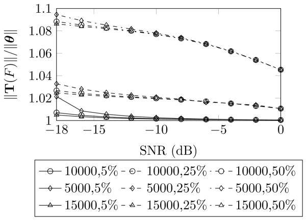
We can investigate ||T(F)||/||θ|| for different SNRs using (13). Q₁ and Q₂ can be evaluated numerically for typical values of p and of contrast variation a and b in cryo-EM (a and b determine F, see (3)). We consider p = 5000, 10000, 15000 which loosely correspond to images of size 64×64, 100×100 and 128 × 128. We also consider three ranges of contrast variation: 5% (a = 0.95 and b = 1.05), 25% (a = 0.75 and b = 1.25), and 50% (a = 0.5 and b = 1.5). For each combination of image size p and contrast variation, we numerically evaluated Q₁(p) and Q₂(p), and hence ||T(F)||/||θ|| using (13) for SNRs between −18dB to 0dB. The results are plotted in Fig. 2. The figure shows that the difference between ||T(F)|| and ||θ|| is less than 10% for all values of p and is negligible when amplitude variation is 25% or smaller. Thus, as a close approximation we may regard ||T(F)|| and hence T(F) as consistent.

Fig. 2.

Consistency of ||T(F)||. Image size p = 5000, 10000, 15000 and contrast variation of 5%, 25% and 50% are considered.

D. The Influence Function

We investigate the influence function of the estimator for outliers. The influence function of T(F) is defined as [25]:

$$IF(\mathbf{x};\mathbf{T},F)=\underset{\epsilon \to 0}{lim}\frac{\mathbf{T}(F_{\epsilon })-\mathbf{T}(F)}{\epsilon }=\frac{\partial }{\partial \epsilon }{[\mathbf{T}(F_{\epsilon })]}_{\epsilon =0}$$ (14)

where F_ε = (1 − ε)F + εΔ_x is a contaminated distribution by a point mass at x. Replacing F in (7) by F_ε, we have

$$[\int w(\mathbf{y},\mathbf{T}(F_{\epsilon }))\mathrm{d}{F}_{\epsilon }]\mathbf{T}(F_{\epsilon })=\int \mathbf{y}w(\mathbf{y},\mathbf{T}(F_{\epsilon }))\mathrm{d}{F}_{\epsilon }.$$ (15)

Taking the derivative of both sides of (15) with respect to ε and evaluating at 0 gives

$$\begin{array}{l}w(\mathbf{x},\mathbf{T}(F))\mathbf{T}(F)-\int w(\mathbf{y},\mathbf{T}(F))\mathrm{d}F+\left[\int [w(\mathbf{y},\mathbf{T}(F))+\mathbf{T}(F)\frac{\partial }{\partial \mathbf{t}}{[w(\mathbf{y},\mathbf{t})]}_{\mathbf{T}(F)}]\mathrm{d}F\right]\frac{\partial }{\partial \epsilon }{[\mathbf{T}(F_{\epsilon })]}_{\epsilon =0}\\ =\mathbf{x}w(\mathbf{x},\mathbf{T}(F))-\int \mathbf{y}w(\mathbf{y},\mathbf{T}(F))\mathrm{d}F+\left[\int \mathbf{y}\frac{\partial }{\partial \mathbf{t}}{[w(\mathbf{y},\mathbf{t})]}_{\mathbf{T}(F)}\mathrm{d}F\right]\frac{\partial }{\partial \epsilon }{[\mathbf{T}(F_{\epsilon })]}_{\epsilon =0}.\end{array}$$

Dividing both sides by ∫ w(y, T(F))dF and applying consistency T(F) = θ gives

$$[I-H(\mathit{\theta })]\frac{\partial }{\partial \epsilon }{[\mathbf{T}(F_{\epsilon })]}_{\epsilon =0}=\frac{w(\mathbf{y},\mathit{\theta })(\mathbf{x}-\mathit{\theta })}{\int w(\mathbf{y},\mathit{\theta })\mathrm{d}F},$$

where $H(\mathit{\theta })\triangleq \frac{\int (\mathbf{y}-\mathit{\theta })\frac{\partial }{\partial \mathbf{t}}{[w(\mathbf{y},\mathbf{t})]}_{\mathit{\theta }}}{\int w(\mathbf{y},\mathit{\theta })\mathrm{d}F}$

and H(θ) is a matrix of size p × p (p is the image size). If I − H(θ) is invertible, the influence function is

$$IF(\mathbf{x};\mathbf{T},F)=\frac{\partial }{\partial \epsilon }{[\mathbf{T}(F_{\epsilon })]}_{\epsilon =0}={[\mathbf{I}-H(\mathit{\theta })]}^{-1}\frac{w(\mathbf{x},\mathit{\theta })(\mathbf{x}-\mathit{\theta })}{\int w(\mathbf{y},\mathit{\theta })\mathrm{d}F}.$$

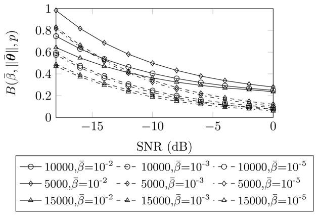
The condition that I − H(θ) is invertible is critical for the existence of the influence function. A simple sufficient condition for I − H(θ) to be invertible is ||H(θ)||_op < 1 where ||·||_op denotes the operator norm. In the Appendix, we show that ||H(θ)||_op ≤ B(β̄, ||θ̄||, p), where β̄ = βσ² with β being the parameter in (6) and σ the standard deviation of image noise. Fig. 3 is a plot of B(β̄, ||θ̄||, p) for the same values of p and SNRs as used in Fig. 2. We consider three values of β̄: 10⁻², 10⁻³, 10⁻⁵ and 50% contrast variation (a = 0.5 and b = 1.5). B is shown as a monotonically decreasing function of SNR. Further, B < 1 for all values of p when β̄ is less than 10⁻³. We use β̄= 10⁻⁵ for all our experiments. Note that this value of β̄ does not need tuning; it may be considered as a fixed constant.

Fig. 3.

Numerical evaluation of B(β̄, ||θ̄||, p). B is evaluated for SNR=−18dB to 0dB (converted from ||θ̄||) and p = 5000, 10000, 15000 and for β̄ = 10⁻², 10⁻³, 10⁻⁵ and 50% contrast variation (a = 0.5 and b = 1.5).

Having established that I − H(θ) is invertible, we can evaluate the influence function for cryo-EM outliers. Recall that an outlier x in cryo-EM has a low correlation coefficient with θ and a finite component along θ. Let the outlier x have a component x₁ ≠ 0 along θ and a component x₂ orthogonal to θ, and the absolute value of the correlation coefficient ϕ = ||x₁||/||x||. We consider the value of the influence function as ϕ → 0:

$$\begin{array}{l}\Vert IF(\mathbf{x};\mathbf{T},F)\Vert =\Vert {[I-H(\mathit{\theta })]}^{-1}\frac{w(\mathbf{x},\mathit{\theta })(\mathbf{x}-\mathit{\theta })}{\int w(\mathbf{y},\mathit{\theta })\mathrm{d}F(\mathbf{y})}\Vert \\ \le \frac{{\Vert {[I-H(\mathit{\theta })]}^{-1}\Vert }_{op}}{\int w(\mathbf{y},\mathit{\theta })\mathrm{d}F(\mathbf{y})}\Vert w(\mathbf{x},\mathit{\theta })(\mathbf{x}-\mathit{\theta })\Vert \\ =K(\mathit{\theta })\Vert w(\mathbf{x},\mathit{\theta })(\mathbf{x}-\mathit{\theta })\Vert ,\end{array}$$ (16)

where K(θ) ≜ ||[I − H(θ)]⁻¹||_op/∫w(y, θ)dF (y). Then

$$\begin{array}{l}\underset{\varphi \to 0}{lim}\Vert w(\mathbf{x},\mathit{\theta })(\mathbf{x}-\mathit{\theta })\Vert =\underset{\varphi \to 0}{lim}\varphi e^{-\beta \frac{(1-{\varphi }^2){\Vert x_1\Vert }^2}{{\varphi }^2}}\sqrt{{\Vert x_1-\mathit{\theta }\Vert }^2+{\Vert x_1\Vert }^2(1-{\varphi }^2)/({\varphi }^2)}\\ =\underset{\varphi \to 0}{lim}{e}^{-\beta \frac{{\Vert x_1\Vert }^2}{{\varphi }^2}}\sqrt{{\varphi }^2{\Vert x_1-\mathit{\theta }\Vert }^2+{\Vert x_1\Vert }^2(1-{\varphi }^2)}=0.\end{array}$$

Further, K(θ) is finite since both ∫w(y, θ)dF (y) and ||[I − H(θ)]⁻¹||_op are finite. Thus, from (16),

$$\underset{\varphi \to 0}{lim}\Vert IF(\mathbf{x};\mathbf{T},F)\Vert \le \underset{\varphi \to 0}{lim}K(\mathit{\theta })\Vert w(\mathbf{x},\mathit{\theta })(\mathbf{x}-\mathit{\theta })\Vert =0.$$

Since the influence function goes to zero when the outliers have zero correlation coefficients with the correct projection and the influence function is continuous, it is also bounded for outliers whose correlation coefficients are small.

IV. Class Mean Estimation for Multiple CTFs

We now turn to the problem of estimating a CTF-corrected class mean from aligned images having different CTFs.

A. Image Model

We assume that each of the N images x_i, i = 1, ···, N has one of L CTFs, c_j, j = 1, ···, L. Let N_j denote the number of images in the j^th CTF group. It will be convenient to use a double index for images, where x_j,k, k = 1, ···, N_j refers to the k^th image in the j^th CTF group.

Assuming Gaussian white noise, the image x_j,k ∈ ℝ^p is

$${\mathbf{x}}_{j,k}=c_j\ast {\mathit{\mu }}_{j,k}+\mathbf{n},$$ (17)

where μ_j,k is the CTF-free non-noisy signal and * denotes the convolution operation.

Inlier

When the image x_j,k is an inlier,

$${\mathit{\mu }}_{j,k}=s\mathit{\mu }$$ (18)

where μ ∈ ℝ^p is the CTF-free non-noisy projection. As before, s models contrast variation and has a uniform density π(s|a, b) where a and b are symmetric about 1. Marginalizing s results in the pdf of inliers x_j,k:

$$f({\mathbf{x}}_{j,k}\mid \mathit{\mu })={\int }_a^{b}g({\mathbf{x}}_{j,k}\mid c_j\ast s\mathit{\mu })\pi (s\mid a,b)\mathrm{d}s$$ (19)

Outlier

Similar to the single-CTF case, for an outlier image:

1. μ_j,k has a low correlation coefficient with μ, and

2. μ_j,k has a finite component along μ.

The goal is to robustly estimate μ from the images.

B. The Robust CTF-corrected Class Mean Estimator

We formulate this estimator in the discrete Fourier transform space where the convolution c_j * μ becomes the point-wise multiplication C_j(s)M (s) where the capital letters denote the 2D discrete Fourier transforms of c_j and μ, and s denotes a point in the 2D discrete Fourier space. C_j(s)M (s) can be written as a matrix operation C_jM, by 1) constructing a diagonal matrix called C_j whose diagonal elements are the components of C_j(s), and 2) scanning M into a column vector.

Our robust CTF-corrected class mean estimate is a weighted version of the estimate in [26] defined as

$$\mathbf{T}={\left[\sum _{j=1}^L{C}_j^T{C}_j{N}_j\right]}^{-1}\left[\sum _{j=1}^L{C}_j^T\sum _{k=1}^{N_j}{\mathbf{X}}_{j,k}\right],$$ (20)

where N_j is the number of images in the j^th CTF group and X_j,k is the discrete Fourier transform of image x_j,k. Note that N_j could take value 1, which simply states that each image has its own CTF. We extend (20) to a robust estimator of the CTF-corrected class mean:

$$\mathbf{T}={\left[\sum _{j=1}^L{C}_j^T{C}_j\sum _{k=1}^{N_j}w({\mathbf{X}}_{j,k},C_j\mathbf{T})\right]}^{-1}\left[\sum _{j=1}^L{C}_j^T\sum _{k=1}^{N_j}w({\mathbf{X}}_{j,k},C_j\mathbf{T}){\mathbf{X}}_{j,k}\right]$$ (21)

by incorporating the weight function w(X, T) defined in (6).

Similarly, the estimate can be determined by an iterative algorithm.

C. Fisher-Consistency of the Estimator

The Fisher-consistency of T in (21) can be easily shown by applying consistency of the single CTF case to each CTF group. We write T as a statistical functional of F :

$$\mathbf{T}(F)={\left[\sum _{j=1}^L{C}_j^T{C}_j\int w({\mathbf{X}}_j,C_j\mathbf{T}(F))\mathrm{d}{F}_j({\mathbf{X}}_j)\right]}^{-1}·\left[\sum _{j=1}^L{C}_j^T\int w({\mathbf{X}}_j,C_j\mathbf{T}(F)){\mathbf{X}}_j\mathrm{d}{F}_j({\mathbf{X}}_j)\right],$$ (22)

where X_j denotes the image in the j^th CTF group and F_j is the distribution of X_j. T(F) is Fisher-consistent if T(F) = M where M is the Fourier transform of μ.

From the consistency of the single CTF case,

$$\begin{array}{l}{C}_{j}M=\frac{\int w({\mathbf{X}}_j,C_{j}M){\mathbf{X}}_j\mathrm{d}{F}_j({\mathbf{X}}_j)}{\int w({\mathbf{X}}_j,C_{j}M)\mathrm{d}{F}_j({\mathbf{X}}_j)},\text{which}\text{gives}\\ C_{j}M\int w({\mathbf{X}}_j,C_{j}M)\mathrm{d}{F}_j=\int w({\mathbf{X}}_j,C_{j}M){\mathbf{X}}_j\mathrm{d}{F}_j.\end{array}$$

Multiplying both sides by $C_j^T$ and summing over all js,

$$\sum _{j=1}^L\left[C_j^T{C}_j\int w({\mathbf{X}}_j,C_{j}M)\mathrm{d}{F}_j\right]M=\sum _{j=1}^L{C}_j^T\int w({\mathbf{X}}_j,C_{j}M){\mathbf{X}}_j\mathrm{d}{F}_j.$$

Rearranging the terms,

$$\begin{array}{l}M={\left[\sum _{j=1}^L{C}_j^T{C}_j\int w({\mathbf{X}}_j,C_{j}M)\mathrm{d}{F}_j\right]}^{-1}\\ ·\left[\sum _{j=1}^L{C}_j^T\int w({\mathbf{X}}_j,C_{j}M){\mathbf{X}}_j\mathrm{d}{F}_j\right].\end{array}$$ (23)

Comparing (23) and (22) shows that T(F) = M.

D. The Influence Function

In this section we derive the influence function of the estimator and show that it is bounded for outliers. We evaluate the influence function for an outlier X as its correlation coefficient with the CTF-affected projection Θ goes to zero while the component of X along Θ remains finite (Θ = CM where C is the CTF of the outlier image X).

The influence function of T in (22) at a distribution F is calculated by $IF(\mathbf{X};\mathbf{T},F)=\frac{\partial }{\partial \epsilon }{[\mathbf{T}(F_{\epsilon })]}_{\epsilon =0}$, where F_ε is a contaminated distribution by putting a ε mass at one of the distributions F_j, j = 1, ···, L of CTF group. Let the k^th CTF group be this contaminated CTF group and denote the contaminated distribution F_{k_ε} = (1 − ε)F_k + εΔ_X. The influence function can then be derived by replacing F by F_ε in (22), taking derivative of (22) with respect to ε and evaluating at 0 and applying the consistency T(F) = M, which gives

$$[I-Z(M)]\frac{\partial }{\partial \epsilon }{[\mathbf{T}(F_{\epsilon })]}_{\epsilon =0}={\left[\sum _j{C}_j^T{C}_j\int w({\mathbf{Y}}_j,C_{j}M)\mathrm{d}{F}_j\right]}^{-1}·C_k^{T}w(\mathbf{X},C_{k}M)(\mathbf{X}-C_{k}M),$$

where $Z(M)\triangleq {\left[{\displaystyle \sum _j}{C}_j^T{C}_j\int w({\mathbf{Y}}_j,C_{j}M)\mathrm{d}{F}_j\right]}^{-1}·\left[{\displaystyle \sum _j}{C}_j^T\int ({\mathbf{Y}}_j-C_{j}M)\frac{\partial }{\partial \mathbf{t}}{[w({\mathbf{Y}}_j,\mathbf{t})]}_{C_{j}M}\mathrm{d}{F}_j{C}_j\right]$.

If I − Z(M) is invertible, then the influence function is

$$IF(\mathbf{x};\mathbf{T},F)={\left[(\sum _j{C}_j^T{C}_j\int w({\mathbf{Y}}_i,C_{j}M)\mathrm{d}{F}_j)(I-Z(M))\right]}^{-1}·C_k^{T}w(\mathbf{X},C_{k}M)(\mathbf{X}-C_{k}M).$$

I − Z(M) has to be invertible for the existence of the influence function. Using the results of the single CTF case, we prove in the appendix the following sufficient condition: B(β̄, ||Θ̄||, p) < 1,∀1 ≤ j ≤ L, where B(β̄, ||Θ̄||, p) is derived in the single CTF case and β̄ = βσ², Θ̄ = Θ/σ. Such a condition can be satisfied by choosing proper β̄. We have shown in Section III-D that for relevant ||Θ̄|| and p, β̄ = 10⁻⁵ satisfies the condition.

We next evaluate the influence function for outliers X. Let X = [X₁, X₂]^T where X₁ and X₂ are along and orthogonal to Θ_k = C_kM. Similarly, we consider the influence function as ϕ ≜ ||X₁||/||X|| goes to zero while ||X₁|| is finite. First,

$$\begin{array}{l}\Vert IF(\mathbf{X};\mathbf{T},F)\Vert \le K(M)\Vert C_k^{T}w(\mathbf{X},C_{k}M)(\mathbf{X}-C_{k}M)\Vert ,\\ K(M)\triangleq {\Vert {\left[({\sum }_j{C}_j^T{C}_j\int w({\mathbf{Y}}_i,C_{j}M)\mathrm{d}{F}_j)(I-Z(M))\right]}^{-1}\Vert }_{op}.\end{array}$$

Since K(M) is also finite, lim_ϕ→0 ||IF (X; T, F)||

$$\le \underset{\varphi \to 0}{lim}K(M)\Vert w(\mathbf{X},C_{k}M)(\mathbf{X}-C_{k}M)\Vert =0.$$

Thus the estimator for the CTF-corrected class-mean also has a zero influence function for outliers.

V. Experimental Results

We present the results of our estimator applied to simulated and real cryo-EM images.

A. Simulated Data

Simulated cryo-EM images were generated from the atomic structure of the 50S ribosomal subunit from the Protein Data Bank (PDB ID: 1JJ2) using a hydration model [27], and was sampled at a pixel size of 3Å. The 2D particle images (inliers) were obtained from the 3D structure according to the image model in (17) and (18) by: 1) projecting the structure and applying a CTF; 2) applying the amplitude factor from a uniform distribution between 0.5 and1.5; and 3) adding Gaussian white noise.

To model the outliers in cryo-EM, we followed a strategy reported in [28] and generated a uniform mixture of images from five classes: misclassified images, projection of a sphere, a plane and a cylinder, and pure noise image. Misclassified images are projections from other directions than the inliers with the difference of the projection directions larger than 65 degrees. Fig. 4 shows typical images from these five classes of outliers. CTF, amplitude variation and Gaussian white noise were also applied to these projections in the same way as for the inliers.

Fig. 4.

Simulated outliers. Examples of non-noisy outliers (top row) and their CTF-affected and noisy version (bottom row), including (from left to right) a misaligned particle, projection of a sphere, a plane, a cylinder and image of pure noise.

For the single CTF case, a CTF with defocus 1.3μm was used. For multiple CTF case, five CTFs with defocus values 1.0μm, 1.8μm, 2.0μm, 2.8μm and 3.5μm were used.

B. Cryo-EM Data

Real cryo-EM images were the 50S ribosomal subunit images from the National Resource for Automated Molecular Microscopy. Images were classified into five CTF groups (defocus of 1.2μm, 1.6μm, 1.9μm, 2.2μm and 2.5μm) and aligned by the software package SPIDER [8].

C. Performance Measures

We measured the ability of the proposed w-estimator (referred to as wme) to reject outliers and compared it with the classical cross-correlation with thresholds (referred to as cc). We use two figures of merit: the precision rate (P) and the recall rate (R). For an outlier detection method that makes hard decision about whether an observation is an outlier or not, P and R are calculated by:

$$P=\frac{TP}{TP+FP}R=\frac{TP}{TP+FN},$$ (24)

where TP, FP, TN and FN are the number of true positives (correctly classified inliers), false positives (outliers misclassified as inliers), true negatives (correctly classified outliers) and false negatives (inliers misclassified as outliers) [29]. The precision rate measures the fraction of images which participate in the averaging step that are inliers. The recall rate measures the fraction of inliers included in averaging with respect to all available inliers. Since the w-estimator does not make hard decision about outliers but rather assigns weights to the outliers, we calculate two equivalent metrics to P and R:

$$\widehat{P}=\frac{{\sum }_{j\in S}{w}_j}{{\sum }_j{w}_j}\widehat{R}=\frac{{\sum }_{j\in S}min(1,\frac{w_j}{{\sum }_i{w}_i}{N}_{in})}{N_{in}}$$ (25)

where w_j are the image weights, S contains indices of inliers and N_in is the cardinality of S. P̂ measures the contribution of inliers to the averaging and is thus equivalent to P in (24). The numerator of R̂ calculates the equivalent number of TP by examining the contribution of each inlier that participates in the averaging. Since TP + FN = N_in, R̂ is equivalent to R in (24).

A second criterion that we used for performance comparison is the standard deviations of the precision and recall rates, which characterize the consistency of the performance.

Finally, to assess the accuracy of the resulting class means, we calculated the mean square error between the class means and the non-noisy projection in different frequency rings.

D. Results for single CTF Class Means

1) Simulations

Before presenting the results for the precision and recall rates, we first demonstrate that the w-estimator works as designed, i.e. at convergence it down-weighs the contribution of the outliers to the class mean. We took a total of 30 images, 12 of which are outliers (40% outliers). In cryo-EM, the number of images per direction goes up to the order of 100. We chose to report results with vastly fewer images because this is the more challenging case (a significant amount of noise remains in the estimated class mean). Noise was added to create an SNR of −16dB.

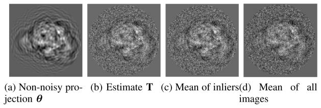
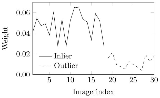
Fig. 5 shows the non-noisy projection, the w-estimate, the mean of inliers and the mean of all images. The w-estimate is close to the mean of inliers. Fig. 6 shows the converged weights of images. Note that the weights of the outliers are on average lower than 20% of the weights of the inliers, showing that the effect of outliers on the estimate is greatly diminished.

Fig. 5.

Results for simulated data in the single CTF case. (a) shows the non-noisy projection θ. (b), (c) and (d) are the w-estimate T, the mean of inliers and the mean of all images.

Fig. 6.

Weights of the images at convergence for simulated data in the single-CTF case. 30 images with 40% of outliers with SNR of −16dB.

To continue, we compared the performance of wme with that of cc using precision and recall rates. We evaluated the performances for different SNRs and different outlier percentages.

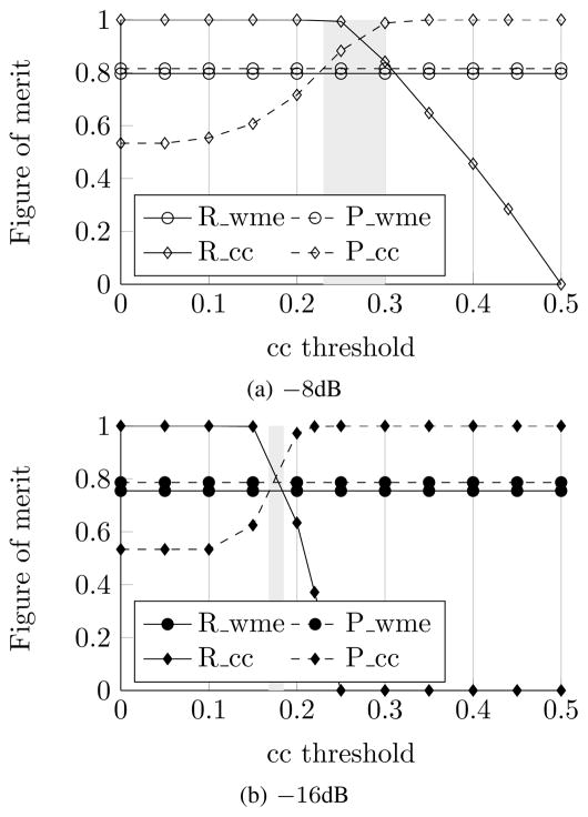
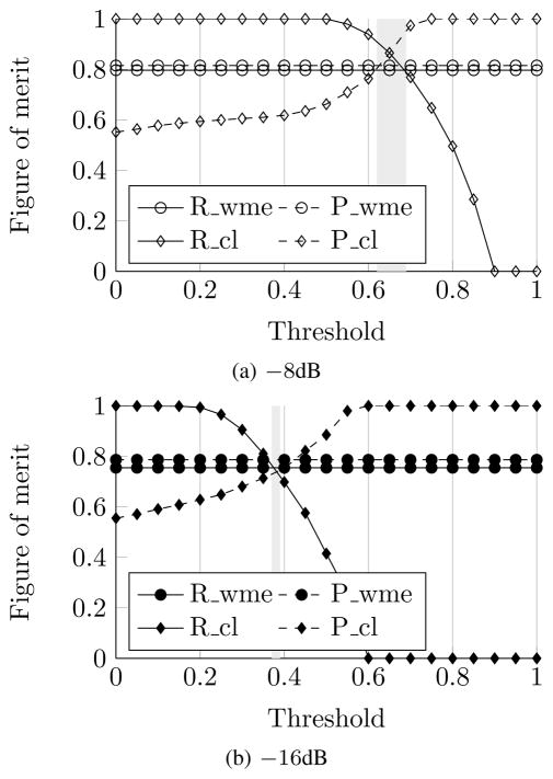
First, we evaluated wme and cc on images that represent the typical highest and lowest SNRs observed in cryo-EM: −8dB and −16dB. A total of 30 images of each SNR were generated, both with 45% of outliers. This was repeated 100 times. Fig. 7 a–b shows the mean values of the precision (P) and recall (R) rates for wme and cc for SNR −8dB and −16dB respectively. P and R for cc depend on threshold, which is indicated on the x-axis with varying thresholds. The wme does not require a threshold and its rates are shown as horizontal lines. Two observations can be made from Fig. 7: 1) for both noise levels, there is a very small range of thresholds (denoted as shaded area) in which the cc performance is comparable to the wme performance. The performance of cc degrades rapidly when the threshold falls out of this range, with either P or R falling off from its high value. 2) The aforementioned ranges for the two SNRs are very different from each other. This clearly shows that the threshold has to be adjusted for images of different SNRs. In contrast, wme naturally adapts to different SNRs without requiring any manual adjustment. The standard deviations of P and R for wme and cc are shown in Table I where cc was evaluated with the optimal threshold (e.g., 0.18 is used for images of −16dB since Fig. 7b shows that it generates the best performance). The wme demonstrates consistently smaller standard deviations than cc, further supporting the claim that it reliably reduces the influence of outliers even when the SNR changes.

Fig. 7.

Performance of cross-correlation with thresholds (cc) and the proposed w-estimator (wme) at two signal-to-noise ratios (SNR): (a) −8dB and (b) −16dB. 45% outliers are present in both cases. P and R are the precision and recall rates.

TABLE I.

Standard deviation of precision and recall rates of cross-correlation with thresholds (cc) and the w-estimator (wme) in the single CTF case.

	−8 dB		−16 dB
	cc1	wme	cc2	wme
Precision	0.07	0.03	0.09	0.04
Recall	0.04	0.02	0.08	0.03

¹at threshold of 0.27

²at threshold of 0.18

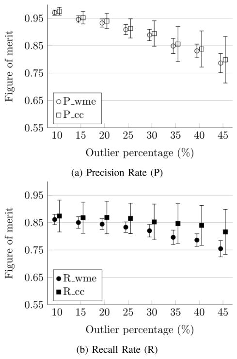
Second, we compared the performances of wme and cc for data with different outlier percentages. The precision and recall rates are calculated for data containing 10% to 45% outliers with SNR −16dB. The thresholds used in evaluating the performance of cc are the values that generate the best performance. Fig. 8 shows the mean and standard deviation of the rates for wme and cc, calculated from 100 experiments for each outlier percentage. The wme is shown to have comparable rates to those of cc while the standard deviations of the rates for wme are consistently lower for all outlier percentages, demonstrating the reliability of wme performance.

Fig. 8.

Performance of cross-correlation with thresholds (cc) and the proposed w-estimator (wme) to varying outlier percentages. Optimal thresholds are used for cc. (a) and (b) show the result of precision rate (P) and recall rate (R) respectively. 10% to 45% outliers and SNR of −16dB.

To further compare the quality of the class means and to understand the effects of outliers, we calculated the mean squared error (MSE) between the class means and the non-noisy projection in frequency rings. Similar to calculating Fourier ring correlation (FRC) [30], the MSE between the Fourier-transformed class means and non-noisy projection was computed for concentric rings of increasing radius centered at (0, 0) frequency. Fig. 9a shows the MSE of wme, the classical mean (no outlier removal) and cc with different thresholds (0.18 is the optimal threshold). We used a total of 30 images with SNR −16dB and 45% outliers and results were calculated from 100 repeated experiments. Several observations can be made: 1) The MSE at around 1/200Å⁻¹ are comparably high for all methods since CTF causes loss of low frequency information. 2) The classical mean and cc with thresholds 0.16 and 0.18 all have higher MSE between 1/200Å⁻¹ and 1/31.6Å⁻¹ which is the range of frequencies within the first peak of the corresponding CTF (Fig. 9b). This range of frequencies is where the outliers have the most influence. 3) For cc, small deviation from the optimal threshold causes the MSE to increase, showing that the performance of cc is very sensitive to thresholds. 4) The low MSE of the wme estimate in lower frequency regions shows that it outperforms cc and the classical mean. (The MSE of the classical mean and cc with threshold 0.16 are slightly lower than wme in higher frequency regions, because they average more images and only noise is present in these regions.)

We also compared the performance of wme with the common-lines (cl) based approach in [16]. Two sets of 900 class means from uniform projections of the north hemisphere of the simulated 50S ribosome subunit were generated, with SNRs equivalent to averaging 30 images with SNRs of −8dB and −16dB. Along one projection direction, 30 images (SNRs of −8dB or −16dB) with 45% outliers were created. Their common-line projection correlation coefficient with all of the class means from the remaining 899 directions were calculated and used for outlier rejection. Fig. 10 shows the mean precision and recall rates from 100 repeated experiments. The results show that the performance of correlating the common-lines is also sensitive to the choice of thresholds, and wme has performance comparable to the best common-lines performance where the “optimal” threshold (gray area) is used.

Fig. 10.

Performance of common-line based approach (cl) and the proposed w-estimator (wme) at two signal-to-noise ratios (SNR): (a) −8dB and (b) −16dB. A total of 900 common-lines and 45% outliers. P and R are the precision and recall rates.

2) Real Cryo-EM Images

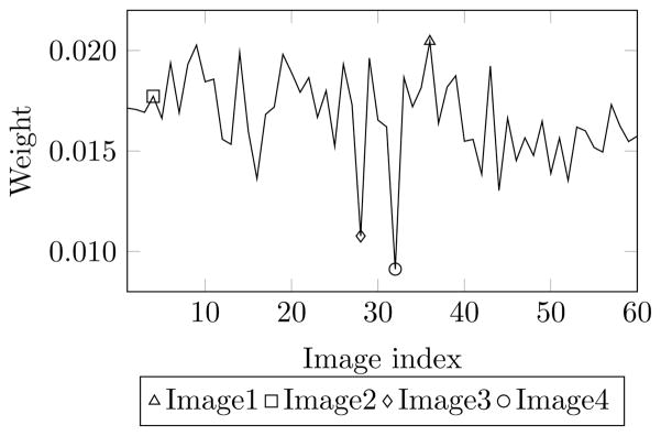
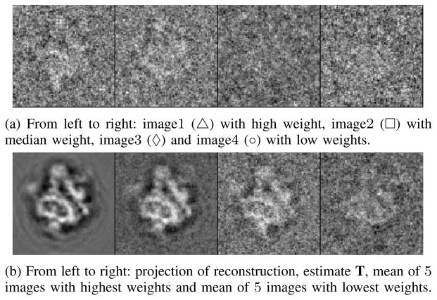
We next show the results on real cryo-EM data. Sixty images of 50S Ribosome subunit aligned to a projection direction from CTF5 group (highest defocus) were used. Fig. 11 shows the converged weights of wme. Notice that two images have significantly lower weights. To further assess the quality of these images, we chose to examine four images (denotes as Image1-4 in Fig. 11): Image1 with a high weight, Image2 with median weight, and Image3 and Image4 with lower weights. Fig. 12a displays these four images. The projection of the reconstruction obtained by the algorithm in [31] serves as a reference for the non-noisy projection of the particle and is shown in Fig. 12b. Comparing the images in Fig. 12a with the reference in Fig. 12b strongly suggests that the two images with lower weights do not appear to contain the signal of the projected structure. To further confirm this, we took 5 images with the highest and lowest converged weights and calculate the mean images from them. The resulting mean images, displayed in Fig. 12b, show that the images with lowest weights contain signal different from the projected structure and the rest of the images. Fig. 12b also shows the estimate of the class-mean from our estimator.

Fig. 11.

Weights of images at convergence for cryo-EM images. Four images are labeled: image1 (△) with high weight, image2 (□) with median weight, image3 (◇) and image4 (○) with low weights.

Fig. 12.

Results for cryo-EM images in the single CTF case.

To summarize, experiments with the single CTF case have shown that: 1) the performance of cross-correlation is sensitive to the threshold and has to be adjusted for images of different SNRs. 2) the w-estimator performs as well as the cross-correlation (with optimal threshold) without the need of adjustment for varying SNRs and outlier percentages. 3) w-estimator is able to down-weight outliers in real cryo-EM case.

E. Results for Multiple CTF Class Means

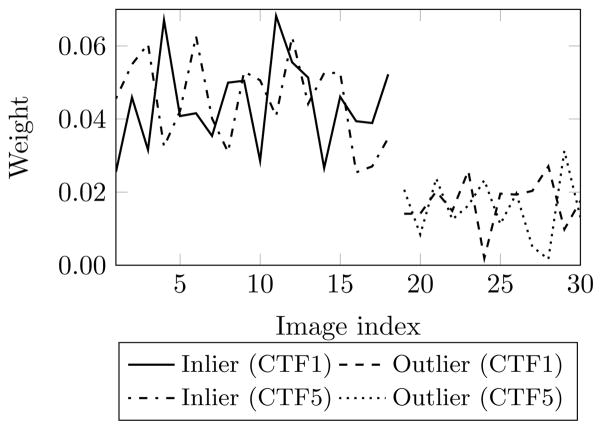
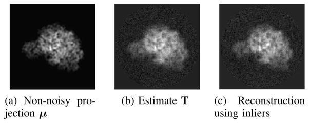
We first show that the proposed w-estimator is capable of handling outliers in more than one CTF groups. 30 images with 40% outliers were generated for each of the five CTF groups. The standard deviation of the image noise is σ = 85 (Because different CTFs lead to different signal energy, the images do not have the same SNRs. This σ corresponds to an average SNR of −15dB.). Fig. 13 shows the converged weights of images for the CTF groups with the smallest (CTF1) and largest (CTF5) defocus values. The weights of other CTF groups have similar behaviors and were omitted in the plot for ease of visualization. For the same reason, the weights shown in Fig. 13 are normalized such that the weights of all images within each CTF group sum up to 1. For all CTF groups, the weights of the outliers are lower than 20% of the weights of the inliers. Fig. 14 shows the CTF-free non-noisy projection, the estimate from the w-estimator and the estimate from a hypothetical “ideal” method that uses equal weights for inliers and zero weights for outliers. The w-estimate is similar to the class mean produced by the ideal method.

Fig. 13.

Weights of images at convergence for simulated images in the multiple CTF case. Results of CTF1 (lowest defocus) and CTF5 (highest defocus) are shown. Each CTF group has 40% outliers and average SNR of −15dB. Weights are normalized within each CTF group.

Fig. 14.

Results for simulated data in the multiple CTF case. (a) shows the non-noisy CTF-free projection μ. (b) is the w-estimate T calculated from the images and (c) is the ideal estimate calculated from the inliers.

Next, we compare the performance of cross-correlation with thresholds (cc) and the w-estimator (wme) for the multiple CTF case. We have already shown from the single CTF case that the performance of cc is sensitive to threshold for varying SNRs. For the multiple CTF case, cc is performed independently for each CTF group. Fig. 15 shows the precision and recall rates of wme and cc. Results of two CTF groups with defocus values of 1.0μm and 3.5μm are shown. The shaded area in the two plots indicate the range of thresholds within which the performance of cc is comparable to wme. These ranges are narrow for both CTF groups and the two ranges have very limited overlapping region. This is evidence that the same threshold cannot be used for all CTF groups. In contrast, wme achieves satisfactory performance for different CTF groups without adjustments.

Fig. 15.

Performance of cross-correlation with thresholds (cc) and the w-estimator (wme) for multiple-CTF case. cc is performed independently for each CTF groups. Precision (P) and Recall (R) rates of two CTFs with defocus values of: (a) 1.0μm and (b) 3.5μm are shown. 40% outliers.

We next show that wme for the multiple CTF case also adapts to varying SNRs and outlier percentages. We calculated the precision and recall rates of wme and cc for data with combinations of two SNRs (−7dB and −15dB) and two outlier percentages (10% and 40%). The rates and their standard deviations are reported in Table II. We included the results of wme for both single CTF (wme(s), i.e. applying wme independently for each CTF group) and multiple CTF (wme(m)). For both wme(s) and wme(m), their rates are comparable to cc but with much lower standard deviations. The performance of wme(m) is on average better than wme(s), wme(m) uses images from more than one CTF.

TABLE II.

Precision rate and recall rate and their standard deviations of the w-estimator for single (wme(s)) and multi CTF (wme(m)) cases and cross-correlation with thresholds (cc) in the multiple CTF case.

10% outlier	−7dB			−15dB
	cc	wme(s)	wme(m)	cc	wme(s)	wme(m)
Precision	0.98(0.02)	0.97(0.01)	0.97(0.01)	0.96(0.03)	0.96(0.01)	0.96(0.01)
Recall	0.91(0.05)	0.89(0.01)	0.89(0.01)	0.88(0.06)	0.86(0.02)	0.87(0.02)
40% outlier	−7dB			−15dB
	cc	wme(s)	wme(m)	cc	wme(s)	wme(m)
Precision	0.86(0.07)	0.84(0.03)	0.84(0.02)	0.78(0.07)	0.80(0.03)	0.81(0.03)
Recall	0.82(0.06)	0.83(0.02)	0.83(0.02)	0.80(0.08)	0.78(0.03)	0.78(0.03)

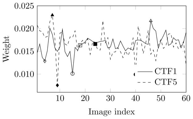
Finally, we show results of real cryo-EM images with five CTF groups, each having 60 images. Fig. 16 shows the converged weights for CTF1 (smallest defocus) and CTF5 (largest defocus) groups. For both groups, four images were chosen: an image with a high weight, an image with a median weight and two images with lower weights. Top and bottom rows of Fig. 17a shows images in CTF1 and CTF5. The projection of the reconstruction is given in Fig. 17b. The images with low weights of CTF5 do not appear to contain the same particle signal as the images with higher weights; the images with low weights of CTF1 appear to contain minimal signals.

Fig. 16.

Weights of images at convergence for cryo-EM images. Results of CTF1 (lowest defocus) and CTF5 (highest defocus) are shown. Weights are normalized within each CTF group. Four images are labeled for each CTF group: image1 (△/▲) with high weight, image2 (□/■) with median weight, image3 (◇/◆) and image4 (○/●) with low weights.

Fig. 17.

Results for cryo-EM images in the multiple CTF case. (a) shows the images from two CTF groups that are labeled in Fig. 16. From left to right: image1 (△/▲) with high weight, image2 (□/■) with median weight, image3 (◇/◆) and image4 (○/●) with low weights. (b) is the projection of the reconstruction.

VI. Conclusion and Discussion

We presented a new approach to estimate class means in the presence of outliers in cryo-EM. The new estimator is applied to the images after they are aligned according to their projection directions and CTFs. Instead of attempting to reject outlier images with a threshold, this approach aims to calculate the class means by a weighted average of images where the weight function limits the influence of outliers. The estimator is robust against outliers; its influence function is bounded and goes to zero asymptotically.

Classical methods for outlier detection require a manually adjusted threshold, such as a threshold for the correlation coefficient. Simulations show that performance of such methods is very sensitive to the choice of threshold. Optimal thresholds are also difficult to find in practice. The main advantage of our approach is that it eliminates thresholds and automatically adapts to the SNR and the outlier percentage of the data.

We also extended the proposed estimator to multiple CTFs. This estimator is capable of estimating the CTF-corrected class mean while limiting the effects of outliers. Experiments with simulated data demonstrate its ability to deal with outliers in more than one CTF group.

We applied the estimator to experimental cryo-EM data of 50S ribosomal subunit. For both single and multiple CTF cases, the estimator assigns lower weights to possible outlier images and limits their influence of on the class means.

The proposed estimator calculates robust 2D class means when outliers are present, by using the weighting scheme of the w-estimators. Such a strategy can be adopted for robust 3D reconstruction by incorporating weights in the reconstruction calculation. Although weighted reconstruction were proposed in [17] and [14], they either do not address the outliers or require heuristics in choosing the parameter values. By posing reconstruction as a robust estimation problem and designing an estimator with desired properties, images from all projection directions can be used for a robust 3D reconstruction.

The robust estimation framework proposed in this work is also useful for other image processing problems. One possible application is robustifying the non-local means (NLM) algorithm [32] for image denoising. The performance of NLM can be improved by using weight functions similar to one proposed here.

Biographies

Chenxi Huang Chenxi Huang is a Ph.D. student in the Department of Biomedical Engineering at Yale University. She received her B.E. of Information Engineering from Shanghai Jiaotong University and M.S. of Electrical Engineering from Yale University. Her research interests are mathematical and computational approaches to biomedical data analysis.

Hemant D. Tagare Hemant D. Tagare is a Professor in the Department of Diagnostic Radiology, the Department of Biomedical Engineering, and the Department of Electrical Engineering at Yale University. He received his Ph.D. from Rice University. His research interests are in bio-medical signal and image analysis. He is a senior member of IEEE.

Appendix A Proof of Claim 1

First, using Cauchy-Schwarz inequality, $E_{\mathbf{x}}[\Vert \mathbf{x}h(\mathbf{x})\Vert ]=\int \Vert \mathbf{x}\Vert h(\mathbf{x})f(\mathbf{x})\mathrm{d}\mathbf{x}\le \sqrt{\int {\Vert \mathbf{x}\Vert }^{2}f(\mathbf{x})\mathrm{d}\mathbf{x}}\sqrt{\int h{(\mathbf{x})}^{2}f(\mathbf{x})\mathrm{d}\mathbf{x}}$. Since ∫ h(x)²f(x)d ≤ M² (h(x) ≤ M and ∫ f(x)dx = 1) and ∫ ||x||²f(x)dx = Q² < ∞, E_x[||xh(x)||] ≤ QM < ∞. Thus ||E_x[xh(x)]|| ≤ E_x[||xh(x)||] < ∞. Consider two cases:

1. p = 1. h(x) is an even function, i.e., h(−x) = h(x). Then $E_x[xh(x)]={\int }_{-\infty }^{\infty }xh(x)f(x)\mathrm{d}x={\int }_0^{\infty }xh(x)[f(x)-f(-x)]\mathrm{d}x$. Also, if x > 0, f(x) > f(−x) hence E_x[xh(x)] > 0 when θ > 0 and f(x) < f(−x) hence E_x[xh(x)] < 0 when θ < 0. Thus, E_x[xh(x)] = αθ where α > 0.

2. p > 1. Let x = [x₁, x_1̃], where x_1̃ denotes the vector containing the second to the p^th components. Let θ = [θ, 0]. Then x₁ ~ N(θ, σ²) and x_1̃ ~ N(0, σ²I). Thus E_x1̃|x1[x_1̃h(x)] = 0. Then E_x[x_1̃h(x)] = E_x1[E_x1̃|x1[x_1̃h(x)]] = 0 and E_x[xh(x)] = E_x[x₁h(x)] = E_x1[E_x1̃|x1[x₁h(x)]] = E_x1[x₁E_x1̃|x1[h(x)]] = E_x1[x₁β(x₁)] where β(x₁) ≜ E_x1̃|x1[h(x)]. β(x₁) > 0 except x₁ = 0, and β(x₁) is an even function of x₁. From case 1), E_x1[x₁β(x₁)] = αθ, α > 0. Therefore, E_x[xh(x)] = αθ where α > 0.

Appendix B Upper bound of ||H(θ)||_op

Define a coordinate system where θ = [θ, 0, ···, 0]^T and y = [y₁, ···, y_p]^T. We have f(y) = f(y₁|θ)f(y₂) ··· f(y_p) where $f(y_1\mid \theta )={\int }_a^{b}1/(b-a)g(y_1\mid s\theta )\mathrm{d}s$ and f(y_i) = g(y_i|0), i = 2, ···, p. g(y|γ) is the pdf of N(γ, σ²).

Let $U(\mathit{\theta })=\int (\mathbf{y}-\mathit{\theta })\frac{\partial }{\partial \mathbf{t}}[w(\mathbf{y},\mathbf{t})]{\mid }_{\mathit{\theta }}\mathrm{d}F$ and V(θ) = ∫ w(y, T(F))dF. U(θ) is a diagonal matrix with components

$$a_{jj}=\int y_i[sgn(y_1)\frac{y_j{e}^{-\beta {\sum }_2^p{y}_i^2}}{\Vert \mathbf{y}\Vert \Vert \mathit{\theta }\Vert }(1+2\beta y_1^2)]\mathrm{d}F.$$

Furthermore, a_jj are identical except a₁₁ = 0. An upper bound of a_jj can be derived as follows:

Let $\overline{\mathbf{y}}=\frac{\mathbf{y}}{\sigma },\overline{\mathit{\theta }}=\frac{\mathit{\theta }}{\sigma }$, β̄ = βσ² and f^*(ȳ₁) = f(ȳ₁) − f(−ȳ₁).

$$\begin{array}{l}{a}_{jj}=\int {\int }_0^{\infty }{e}^{-\overline{\beta }{\sum }_2^p{\overline{y}}_i^2}\frac{{{\overline{y}}_j}^2(1+2\overline{\beta }{\overline{y}}_1^2)}{\Vert \overline{\mathbf{y}}\Vert \Vert \overline{\mathit{\theta }}\Vert }{f}^{\ast }({\overline{y}}_1)\mathrm{d}{\overline{y}}_1\prod _2^{p}f({\overline{y}}_i)\mathrm{d}{\overline{y}}_i\\ \le \int {\int }_0^{\infty }{e}^{-\overline{\beta }{\sum }_2^p{\overline{y}}_i^2}\frac{\mid {\overline{y}}_j\mid (1+2\overline{\beta }{\overline{y}}_1\mid {\overline{y}}_j\mid )}{\Vert \overline{\mathit{\theta }}\Vert }{f}^{\ast }({\overline{y}}_1)\mathrm{d}{\overline{y}}_1\prod _2^{p}f({\overline{y}}_i)\mathrm{d}{\overline{y}}_i\\ =Q_1(\overline{\beta },\Vert \overline{\mathit{\theta }}\Vert )\prod _{i\ne 1,j}{e}^{-\overline{\beta }{\sum }_{i\ne 1,j}^p{\overline{y}}_i^2}f({\overline{y}}_i)\mathrm{d}{\overline{y}}_i,\end{array}$$ (26)

$$Q_1(\overline{\beta },\Vert \overline{\mathit{\theta }}\Vert )\triangleq \int {\int }_0^{\infty }{e}^{-\overline{\beta }{\overline{y}}_j^2}\frac{\mid {\overline{y}}_j\mid (1+2\overline{\beta }{\overline{y}}_1\mid {\overline{y}}_j\mid )}{\Vert \overline{\mathit{\theta }}\Vert }{f}^{\ast }({\overline{y}}_1)f({\overline{y}}_j)\mathrm{d}{\overline{y}}_1\mathrm{d}{\overline{y}}_j.$$

Evaluating (26) in spherical coordinates and let $C(p)\triangleq {(\frac{1}{\sqrt{2\pi }})}^{p-2}\int sin{\varphi }_1\cdots sin{\varphi }_{p-3}\mathrm{d}{\varphi }_1\cdots \mathrm{d}{\varphi }_{p-3}$,

$$\begin{array}{l}{\Vert U(\mathit{\theta })\Vert }_{op}\le C(p)Q_1(\overline{\beta },\Vert \overline{\mathit{\theta }}\Vert ){\int }_0^{\infty }{e}^{-(\overline{\beta }+\frac{1}{2})r^2}{r}^{p-3}\mathrm{d}r\\ =C(p)Q_1(\overline{\beta },\Vert \overline{\mathit{\theta }}\Vert )\frac{\mathrm{\Gamma }(\frac{p-2}{2})}{2{(\overline{\beta }+\frac{1}{2})}^{\frac{p-2}{2}}}.\end{array}$$

Similarly, a lower bound of V(θ) can be derived as:

$$\begin{array}{l}V(\mathit{\theta })=\int [\int \int e^{-\overline{\beta }{\overline{y}}_j}\frac{\mid {\overline{y}}_1\mid }{\Vert \overline{\mathbf{y}}\Vert }f({\overline{y}}_1)f({\overline{y}}_j)\mathrm{d}{\overline{y}}_1\mathrm{d}{\overline{y}}_j]·\prod _{i\ne 1,j}{e}^{-\overline{\beta }{\sum }_{i\ne 1,j}^p{\overline{y}}_i^2}f({\overline{y}}_i)\mathrm{d}{\overline{y}}_i\\ =C(p){\int }_0^{\infty }[\int \int \frac{e^{-\overline{\beta }{\overline{y}}_j}\mid {\overline{y}}_1\mid f({\overline{y}}_1)f({\overline{y}}_j)}{\sqrt{{\overline{y}}_1^2+{\overline{y}}_j^2+r^2}}\mathrm{d}{\overline{y}}_1\mathrm{d}{\overline{y}}_j]e^{-(\overline{\beta }+\frac{1}{2})r^2}{r}^{p-3}\mathrm{d}r\\ \ge C(p)\int \int \frac{e^{-\overline{\beta }{\overline{y}}_j}\mid {\overline{y}}_1\mid f({\overline{y}}_1)f({\overline{y}}_j)}{\sqrt{{\overline{y}}_1^2+{\overline{y}}_j^2+r_{\mathit{max}}^2}}\mathrm{d}{\overline{y}}_1\mathrm{d}{\overline{y}}_j{\int }_0^{r_{\mathit{max}}}{e}^{-(\overline{\beta }+\frac{1}{2})r^2}{r}^{p-3}\mathrm{d}r\\ =C(p)Q_2(\overline{\beta },\Vert \overline{\mathit{\theta }}\Vert ,r_{\mathit{max}})\frac{\gamma (\frac{p-2}{2},(\overline{\beta }+\frac{1}{2})r_{\mathit{max}}^2)}{2{(\overline{\beta }+\frac{1}{2})}^{\frac{p-2}{2}}},\text{where}\\ Q_2(\overline{\beta },\Vert \overline{\mathit{\theta }}\Vert ,r_{\mathit{max}})\triangleq \int \int \frac{e^{-\overline{\beta }{\overline{y}}_j}\mid {\overline{y}}_1\mid f({\overline{y}}_1)f({\overline{y}}_j)}{\sqrt{{\overline{y}}_1^2+{\overline{y}}_j^2+r_{\mathit{max}}^2}}\mathrm{d}{\overline{y}}_1\mathrm{d}{\overline{y}}_j.\end{array}$$

Define $Q_3(\overline{\beta },\Vert \overline{\mathit{\theta }}\Vert ,p)=\underset{r_{\mathit{max}}}{\text{argmax}}[Q_2(\overline{\beta },\Vert \overline{\mathit{\theta }}\Vert ,r_{\mathit{max}})\gamma (\frac{p-2}{2},(\overline{\beta }+\frac{1}{2})r_{\mathit{max}}^2)],V(\mathit{\theta })\ge C(p)\frac{Q_3(\overline{\beta },\Vert \overline{\mathit{\theta }}\Vert ,p)}{2{(\overline{\beta }+\frac{1}{2})}^{\frac{p-2}{2}}}$. Thus, ${\Vert H(\mathit{\theta })\Vert }_{op}=\frac{{\Vert U(\mathit{\theta })\Vert }_{op}}{V(\mathit{\theta })}\le \frac{Q_1(\overline{\beta },\Vert \overline{\mathit{\theta }}\Vert )\mathrm{\Gamma }(\frac{p-2}{2})}{Q_3(\overline{\beta },\Vert \overline{\mathit{\theta }}\Vert ,p)}\triangleq B(\overline{\beta },\Vert \overline{\mathit{\theta }}\Vert ,p)$.

Appendix C Invertibility of I − Z(M)

If $B(\overline{\beta },\Vert \overline{{\mathbf{\Theta }}_j}\Vert ,p)<1$, ∀1 ≤ j ≤ L, then ${\Vert H({\mathbf{\Theta }}_j)\Vert }_{op}\le B(\overline{\beta },\Vert \overline{{\mathbf{\Theta }}_j}\Vert ,p)<1$, where Θ_j = C_jM, which gives

$${\Vert \int ({\mathbf{Y}}_j-C_{j}M)\frac{\partial }{\partial \mathbf{t}}{[w({\mathbf{Y}}_i,\mathbf{t})]}_{C_{j}M}\mathrm{d}{F}_j\Vert }_{op}<\left|\int w({\mathbf{Y}}_j,C_{j}M)\mathrm{d}{F}_j\right|.$$

Further, we have shown $\int ({\mathbf{Y}}_j-C_{j}M)\frac{\partial }{\partial \mathbf{t}}{[w({\mathbf{Y}}_j,\mathbf{t})]}_{C_{j}M}\mathrm{d}{F}_j$ is a diagonal matrix with identical diagonal elements except the first one being zero. Denote this diagonal matrix as diag{0, a_j,, ···, a_j}. Let b_j ≜ ∫ w(Y_j, C_jM)dF_j. Thus |a_j| < |b_j|. C_j are diagonal matrices with elements being the components of the CTF. Let C_j(i) denote its i^th component.

$$\begin{array}{l}A\triangleq \sum _j{C}_j^T\int ({\mathbf{Y}}_j-C_{j}M)\frac{\partial }{\partial \mathbf{t}}{[w({\mathbf{Y}}_j,\mathbf{t})]}_{C_{j}M}\mathrm{d}{F}_j{C}_j\\ =\text{diag}\{0,\sum _j{C}_j^2(2)a_j,\cdots ,\sum _j{C}_j^2(p)a_j\},\text{and}\\ B\triangleq \sum _j{C}_j^T{C}_j\int w({\mathbf{Y}}_j,C_{j}M)\mathrm{d}{F}_j\\ =\text{diag}\{\sum _j{C}_j^2(1)b_j,\cdots ,\sum _j{C}_j^2(p)b_j\}.\end{array}$$

Because Z(M) = B⁻¹A and |a_j| < |b_j| ∀i, ${\Vert Z(M)\Vert }_{op}={max}_i\{\mid {\sum }_j{C}_j^2(i)a_j/{\sum }_j{C}_j^2(i)b_j\mid \}<1$.

References

- 1.Huang C, Tagare H. Robust estimation for class averaging in Cryo- EM Single Particle Reconstruction. 2014 36th Annual International Conference of the IEEE Engineering in Medicine and Biology Society (EMBC); Aug. 2014; pp. 3329–3332. [DOI] [PubMed] [Google Scholar]
- 2.Frank J. Three-Dimensional Electron Microscopy of Macromolecular Assemblies. San Diego: Academic Press; Jan, 1996. [Google Scholar]
- 3.Ramani Lata K, Penczek P, Frank J. Automatic particle picking from electron micrographs. Ultramicroscopy. 1995 Jun;58(34):381–391. doi: 10.1016/0304-3991(95)00002-i. [Online]. Available: http://www.sciencedirect.com/science/article/pii/030439919500002I. [DOI] [PubMed] [Google Scholar]
- 4.Shaikh TR, Trujillo R, LeBarron JS, Baxter WT, Frank J. Particle-verification for single-particle, reference-based reconstruction using multivariate data analysis and classification. Journal of Structural Biology. 2008 Oct;164(1):41–48. doi: 10.1016/j.jsb.2008.06.006. [Online]. Available: http://www.sciencedirect.com/science/article/pii/S1047847708001457. [DOI] [PMC free article] [PubMed] [Google Scholar]
- 5.Nicholson WV, Glaeser RM. Review: Automatic Particle Detection in Electron Microscopy. Journal of Structural Biology. 2001 Feb;133(23):90–101. doi: 10.1006/jsbi.2001.4348. [Online]. Available: http://www.sciencedirect.com/science/article/pii/S1047847701943485. [DOI] [PubMed] [Google Scholar]
- 6.Wong HC, Chen J, Mouche F, Rouiller I, Bern M. Model-based particle picking for cryo-electron microscopy. Journal of Structural Biology. 2004 Jan;145(12):157–167. doi: 10.1016/j.jsb.2003.05.001. [Online]. Available: http://www.sciencedirect.com/science/article/pii/S104784770300296X. [DOI] [PubMed] [Google Scholar]
- 7.Ludtke SJ, Baldwin PR, Chiu W. EMAN: Semiautomated Software for High-Resolution Single-Particle Reconstructions. Journal of Structural Biology. 1999 Dec;128(1):82–97. doi: 10.1006/jsbi.1999.4174. [Online]. Available: http://www.sciencedirect.com/science/article/pii/S1047847799941746. [DOI] [PubMed] [Google Scholar]
- 8.Shaikh TR, Gao H, Baxter WT, Asturias FJ, Boisset N, Leith A, Frank J. SPIDER image processing for single-particle reconstruction of biological macromolecules from electron micrographs. Nature protocols. 2008;3(12):1941–1974. doi: 10.1038/nprot.2008.156. [Online]. Available: http://www.ncbi.nlm.nih.gov/pmc/articles/PMC2737740/ [DOI] [PMC free article] [PubMed] [Google Scholar]
- 9.Heymann JB, Belnap DM. Bsoft: Image processing and molecular modeling for electron microscopy. Journal of Structural Biology. 2007 Jan;157(1):3–18. doi: 10.1016/j.jsb.2006.06.006. [Online]. Available: http://www.sciencedirect.com/science/article/pii/S1047847706001997. [DOI] [PubMed] [Google Scholar]
- 10.Chen JZ, Grigorieff N. SIGNATURE: A single-particle selection system for molecular electron microscopy. Journal of Structural Biology. 2007 Jan;157(1):168–173. doi: 10.1016/j.jsb.2006.06.001. [Online]. Available: http://www.sciencedirect.com/science/article/pii/S1047847706001961. [DOI] [PubMed] [Google Scholar]
- 11.Vargas J, Abrishami V, Marabini R, de la Rosa-Trevn JM, Zaldivar A, Carazo JM, Sorzano COS. Particle quality assessment and sorting for automatic and semiautomatic particle-picking techniques. Journal of Structural Biology. 2013 Sep;183(3):342–353. doi: 10.1016/j.jsb.2013.07.015. [Online]. Available: http://www.sciencedirect.com/science/article/pii/S1047847713001950. [DOI] [PubMed] [Google Scholar]
- 12.Bern M. Model-Based Particle Picking for Cryo-Electron Microscopy. [DOI] [PubMed] [Google Scholar]
- 13.Roseman AM. FindEMa fast, efficient program for automatic selection of particles from electron micrographs. Journal of Structural Biology. 2004 Jan;145(12):91–99. doi: 10.1016/j.jsb.2003.11.007. [Online]. Available: http://www.sciencedirect.com/science/article/pii/S104784770300279X. [DOI] [PubMed] [Google Scholar]
- 14.Grigorieff N. FREALIGN: High-resolution refinement of single particle structures. Journal of Structural Biology. 2007 Jan;157(1):117–125. doi: 10.1016/j.jsb.2006.05.004. [Online]. Available: http://www.sciencedirect.com/science/article/pii/S1047847706001699. [DOI] [PubMed] [Google Scholar]
- 15.Stewart A, Grigorieff N. Noise bias in the refinement of structures derived from single particles. Ultramicroscopy. 2004 Dec;102(1):67–84. doi: 10.1016/j.ultramic.2004.08.008. [Online]. Available: http://www.ncbi.nlm.nih.gov/pubmed/15556702. [DOI] [PubMed] [Google Scholar]
- 16.Shatsky M, Hall RJ, Nogales E, Malik J, Brenner SE. Automated multi-model reconstruction from single-particle electron microscopy data. Journal of Structural Biology. 2010 Apr;170(1):98–108. doi: 10.1016/j.jsb.2010.01.007. [DOI] [PMC free article] [PubMed] [Google Scholar]
- 17.Scheres SHW. RELION: Implementation of a Bayesian approach to cryo-EM structure determination. Journal of Structural Biology. 2012 Dec;180(3):519–530. doi: 10.1016/j.jsb.2012.09.006. [Online]. Available: http://www.sciencedirect.com/science/article/pii/S1047847712002481. [DOI] [PMC free article] [PubMed] [Google Scholar]
- 18.Scheres SH. Maximum-likelihood methods in cryo-EM. Part II: application to experimental data. Methods in enzymology. 2010;482:295–320. doi: 10.1016/S0076-6879(10)82012-9. [Online]. Available: http://www.ncbi.nlm.nih.gov/pmc/articles/PMC3080752/ [DOI] [PMC free article] [PubMed] [Google Scholar]
- 19.Hashem Y, des Georges A, Dhote V, Langlois R, Liao HY, Grassucci RA, Pestova TV, Hellen CUT, Frank J. Hepatitis-C-virus-like internal ribosome entry sites displace eIF3 to gain access to the 40s subunit. Nature. 2013 Nov;503(7477):539–543. doi: 10.1038/nature12658. [Online]. Available: http://www.nature.com/nature/journal/v503/n7477/full/nature12658.html. [DOI] [PMC free article] [PubMed] [Google Scholar]
- 20.Saxton WO, Frank J. Motif detection in quantum noise-limited electron micrographs by cross-correlation. Ultramicroscopy. 1976;2:219–227. doi: 10.1016/s0304-3991(76)91385-1. [Online]. Available: http://www.sciencedirect.com/science/article/pii/S0304399176913851. [DOI] [PubMed] [Google Scholar]
- 21.Frank J, Verschoor A, Boublik M. Computer averaging of electron micrographs of 40s ribosomal subunits. Science (New York, NY) 1981 Dec;214(4527):1353–1355. doi: 10.1126/science.7313694. [DOI] [PubMed] [Google Scholar]
- 22.Zeng X, Stahlberg H, Grigorieff N. A maximum likelihood approach to two-dimensional crystals. Journal of Structural Biology. 2007 Dec;160(3):362–374. doi: 10.1016/j.jsb.2007.09.013. [Online]. Available: http://www.sciencedirect.com/science/article/pii/S1047847707002304. [DOI] [PMC free article] [PubMed] [Google Scholar]
- 23.Sigworth FJ. Classical detection theory and the cryo-EM particle selection problem. Journal of Structural Biology. 2004 Jan;145(12):111–122. doi: 10.1016/j.jsb.2003.10.025. [Online]. Available: http://www.sciencedirect.com/science/article/pii/S1047847703002405. [DOI] [PubMed] [Google Scholar]
- 24.Tukey JW. Exploratory data analysis. Reading, Mass: Addison-Wesley Pub. Co; 1977. [Google Scholar]
- 25.Hampel FR. Robust statistics: the approach based on influence functions. New York: Wiley; 1986. [Google Scholar]
- 26.Ludtke SJ, Jakana J, Song J-L, Chuang DT, Chiu W. A 11.5 single particle reconstruction of GroEL using EMAN1. Journal of Molecular Biology. 2001 Nov;314(2):253–262. doi: 10.1006/jmbi.2001.5133. [Online]. Available: http://www.sciencedirect.com/science/article/pii/S0022283601951332. [DOI] [PubMed] [Google Scholar]
- 27.Shang Z, Sigworth FJ. Hydration-layer models for cryo-EM image simulation. Journal of structural biology. 2012 Oct;180(1):10–16. doi: 10.1016/j.jsb.2012.04.021. [Online]. Available: http://www.ncbi.nlm.nih.gov/pmc/articles/PMC3577369/ [DOI] [PMC free article] [PubMed] [Google Scholar]
- 28.Norousi R, Wickles S, Leidig C, Becker T, Schmid VJ, Beckmann R, Tresch A. Automatic postpicking using MAPPOS improves particle image detection from cryo-EM micrographs. Journal of Structural Biology. 2013 May;182(2):59–66. doi: 10.1016/j.jsb.2013.02.008. [Online]. Available: http://www.sciencedirect.com/science/article/pii/S1047847713000452. [DOI] [PubMed] [Google Scholar]
- 29.Davis J, Goadrich M. The Relationship Between Precision-Recall and ROC Curves. Proceedings of the 23rd International Conference on Machine Learning, ser. ICML ’06; New York, NY, USA: ACM; 2006. pp. 233–240. [Online]. Available: http://doi.acm.org/10.1145/1143844.1143874. [Google Scholar]
- 30.Banterle N, Bui KH, Lemke EA, Beck M. Fourier ring correlation as a resolution criterion for super-resolution microscopy. Journal of Structural Biology. 2013 Sep;183(3):363–367. doi: 10.1016/j.jsb.2013.05.004. [Online]. Available: http://www.sciencedirect.com/science/article/pii/S1047847713001184. [DOI] [PubMed] [Google Scholar]
- 31.Kucukelbir A, Sigworth FJ, Tagare HD. A Bayesian adaptive basis algorithm for single particle reconstruction. Journal of Structural Biology. 2012 Jul;179(1):56–67. doi: 10.1016/j.jsb.2012.04.012. [Online]. Available: http://www.sciencedirect.com/science/article/pii/S1047847712001153. [DOI] [PMC free article] [PubMed] [Google Scholar]
- 32.Buades A, Coll B, Morel JM. A non-local algorithm for image denoising. IEEE Computer Society Conference on Computer Vision and Pattern Recognition, 2005 CVPR 2005; 2 Jun. 2005; pp. 60–65. [Google Scholar]