

Abstract
Multilevel and longitudinal studies are frequently subject to missing data. For example, biomarker studies for oral cancer may involve multiple assays for each participant. Assays may fail, resulting in missing data values that can be assumed to be missing completely at random. Catellier and Muller proposed a data analytic technique to account for data missing at random in multilevel and longitudinal studies. They suggested modifying the degrees of freedom for both the Hotelling-Lawley trace F statistic and its null case reference distribution. We propose parallel adjustments to approximate power for this multivariate test in studies with missing data. The power approximations use a modified non-central F statistic, which is a function of: 1) the expected number of complete cases, 2) the expected number of non-missing pairs of responses, or 3) the trimmed sample size, which is the planned sample size reduced by the anticipated proportion of missing data. The accuracy of the method is assessed by comparing the theoretical results to the Monte Carlo simulated power for the Catellier and Muller multivariate test. Over all experimental conditions, the closest approximation to the empirical power of the Catellier and Muller multivariate test is obtained by adjusting power calculations with the expected number of complete cases. The utility of the method is demonstrated with a multivariate power analysis for a hypothetical oral cancer biomarkers study. We describe how to implement the method using standard, commercially available software products and give example code.
Keywords: balanced linear mixed models, data missing completely at random, Hotelling-Lawley trace power approximation, multilevel and longitudinal studies
1. Introduction
1.1 Balanced linear mixed models for complete and missing data
Mixed models are used often in biomedical research to account for correlations between repeated measures of outcomes, even with missing data. Throughout, we use the term “repeated measures” in the most general sense as multiple measurements of any form taken on a single independent sampling unit. Repeated measurements can be taken across time (longitudinal) or space (spatial), within clusters (multilevel), using different scales (multivariate outcomes), or in designs with combinations of these factors. For convenience, we will call each measurement taken on an independent sampling unit a “unit of observation.” Each independent sampling unit may have several such units of observation.
In this work, we consider the problem of calculating power for experiments which may have outcome data missing completely at random. We limit the discussion to balanced linear mixed models as described by Muller and co-authors [1, 2]. We describe the model for the complete data first, and then explain how the missing data process may affect power calculations.
Muller et al. [1] make the following assumptions about balanced linear mixed models: 1) each independent sampling unit has the same number and choice of response variables, 2) each independent sampling unit has the same covariance structure, and 3) covariates have the same value for the entire independent sampling unit, no matter which unit of observation is considered. Note that we shall relax Assumption 1 shortly to allow for missing data. Assumption 3 corresponds to using a single value of each predictor for each independent sampling unit. This means that the models we consider cannot have time- or space-varying covariates in longitudinal or spatial studies, different treatment assignments within clusters for multilevel studies, or different predictors for various outcome variables in multivariate studies. To clarify the definition of balanced linear mixed models used in this work, we present examples below which include descriptions of study design, study goals, independent sampling units, units of observation and predictors.
An example of a longitudinal study with complete data for which a balanced linear mixed model is appropriate is a study of the shape of the weight gain curve of women during pregnancy. Each woman is measured nine times, on the first day of each month of gestation. Each woman is an independent sampling unit, and the unit of observation is the weight of the woman at each month. We assume that the covariance between the repeated measurements is the same for all women. The model coefficients represent the average weight at each time point, if only an intercept is used as a predictor. Assumption 3 means that the model could include pre-pregnant BMI, which has the same value for each of the nine weight measurements for one participant. If, however, the investigators wished to add a time-varying covariate such as total dietary fat intake measured for each month of gestation for each pregnant woman, a balanced linear mixed model would not be appropriate. The investigators would need a more complex modeling strategy.
An example of a single level, group-randomized trial with complete data for which a balanced linear mixed model is appropriate is a group-randomized trial comparing the effectiveness of two workplace alcohol reduction programs. Here, we assume that each workplace is randomized to one of the two programs, and that the workplace is the independent sampling unit. Each workplace has many workers. The unit of observation is the self-reported average amount of alcohol consumed by each worker in each workplace in the week following the program. The group-randomized trial can be modeled using a balanced linear mixed model if every group (or cluster) includes the same number of participants, if the covariance structure is the same in each workplace, and if the predictors in the model are the same for every worker in a single workplace. In the balanced linear mixed model describing such an experiment, the coefficients are estimates of the average amount of alcohol consumed for each alcohol reduction program. Since workplaces rather than workers are randomized to a program, the main predictor, treatment group, can be used in the balanced linear mixed model. If, however, the investigators wanted to adjust for previous participation in an alcohol reduction program, they would need to use a different modeling strategy since the participation variable has a potentially different value for each worker.
If the workplaces are clustered within neighborhoods, the design becomes a multi-level trial. As long as the same number of workplaces appear in each neighborhood, the correlation between and within workplaces is the same across neighborhoods, and the randomization is at the neighborhood level, the resulting trial can be modeled with a balanced linear mixed model.
The final example, the one for which we present a power analysis in Section 6 of this paper, is a study with multiple outcomes. The goal of the study is to assess the diagnostic value of three oral cancer screening biomarkers, measured on each participant. Here, the study participant is the independent sampling unit, and the unit of observation is the measurement of each biomarker. Each biomarker is sampled from individuals, some with diagnosed cancer of the oral cavity or pharynx (cases) and some with no previous oral cancer diagnoses (controls). The predictors in the model are indicator variables for cases and controls. The study investigator plans to compare biomarker levels between cases and controls and needs to account for the correlation between biomarkers and potentially missing data points. A balanced linear mixed model is appropriate for this study because the same number and type of measurements are taken on each participant, the disease is diagnosed on the level of the participant, and one can assume that the covariance structure of the biomarkers is the same for each participant. The coefficients of the model are the average levels of each biomarker for those with cancer, and those without cancer. When using a balanced linear mixed model, the investigator can include participant level information as predictors or covariates, such as the disease state. However, the investigator would need a different and more complex model if they would like to adjust for a variable measured on the biomarker level.
We have described balanced linear mixed models for experiments with complete data. However, in many longitudinal, spatial, multivariate and multilevel experiments, missing outcome data is common. In this manuscript, we describe power analysis for experiments which when planned, fulfill all the assumptions for a balanced linear mixed model, but when observed, may have missing outcome data. This relaxes assumption 1: the observed experiment may have a different number of units of observation for each independent sampling unit. For the example with women during pregnancy, this means that each woman may have a different number of weight measurements, a subset of the full nine months of weight measurements. For the workplace alcohol treatment experiment, it means that each workplace may have a different number of workers. For the biomarkers example, it means that each study participant may have one, two or three of the biomarker values planned.
We assume that the data is missing completely at random (MCAR) [3] with some constant probability, π. The MCAR assumption means that the chance that each unit of observation is missing is unrelated to observed or unobserved characteristics of the independent sampling unit, or the temporal or spatial details of the unit of observation. The MCAR assumption is appropriate when data are missing due to a random event, such as participants relocating or a failure of the instruments used to conduct the experiment. The assumption is not appropriate if data are missing due to some process that is correlated with the data values themselves. An example of violating the MCAR assumption occurs if an instrument only records values above a certain level or if participants drop out of a therapeutic drug study because the drug worsens symptoms more than placebo. We provide a more formal definition of the missing data process in the methods section.
1.2 Multivariate hypothesis testing for balanced linear mixed models
A standard data analysis approach for studies with multiple correlated outcomes is to use a mixed model Wald test with Kenward-Roger degrees of freedom [4]. The test may be used for studies with either complete or missing data. However, mixed model data analysis using the Wald test has two problems. Depending on the experiment, the models may have a low rate of convergence or an inflated Type I error rate. Convergence problems may occur because of the difficulty of estimating the multiple parameters needed for an unstructured covariance structure (Table I) [2, 5-7]. The observed Type I error rate may exceed the target Type I error rate if the analyst misspecifies the true covariance (Table II) [7]. Inflation occurs in simulation studies even with sample sizes of 100, as in the experiment considered by Gurka et al. [7], shown in Table II. More importantly, Gurka et al. [7] showed mathematically that the inflation can occur with infinitely large sample sizes.
Table I.
Convergence rates for mixed models.
| Study | % Converged |
|---|---|
| Catellier and Muller (2000) | 10 |
| Serrano (2008) | 37 |
| Gurka, Edwards, Muller (2011) | 61 |
| Fouladi and Shieh (2004) | 84 |
Table II.
Type I error for mixed model with correct and incorrect covariance models, α = 0.05, Nt = 100, p = 5, 20% missing data.
| Type I Error | ||
|---|---|---|
| Correlation Model | Correct | Incorrect |
| Autoregressive (AR) | 0.047 | 0.064 |
| Linear in Time | 0.048 | 0.088 |
| Linear in Time & AR | 0.044 | 0.117 |
For balanced linear mixed models with complete outcome data, Muller et al. recommend that researchers choose a multivariate hypothesis test instead of the Wald test. They argue that a multivariate test “always controls test size and has a good power approximation, in sharp contrast to mixed model tests” [1]. In studies with complete outcome data and a balanced design, the mixed model can be recast as a general linear multivariate model and the mixed model Wald test with Kenward-Roger degrees of freedom becomes equivalent to the multivariate Hotelling-Lawley trace test.
Calculation of the Hotelling-Lawley trace statistic requires complete data, limiting the utility of this multivariate approach. To address this gap, Catellier and Muller [2] provided a modification to the Hotelling-Lawley trace test reference distribution. The modification permits the use of the multivariate approach even for studies with missing outcome data, so long as the planned study analysis fits the assumptions for a balanced linear mixed model. The Catellier and Muller [2] approach controls the Type I error rate in many experimental scenarios, even in the presence of missing outcome data.
1.3 Multivariate power approximations for balanced linear mixed models
A multivariate data analysis requires an aligned multivariate power analysis [8]. Current data and power analysis techniques for balanced linear mixed models and multivariate hypothesis tests assume complete data [1]. For analysts facing the possibility of missing outcome data, and choosing to use a Catellier and Muller multivariate test, a new power method is needed. In this work, we propose new power approximations for the Catellier and Muller multivariate test. We compare members of a class of power approximations, and suggest a specific power approximation that yields power values with accuracy to the second decimal place for many common experimental designs with missing data.
In the current work, the new power approximations are described in eight sections. Section 2 contains general notation. Section 3 reviews known methods for data analysis of the balanced linear mixed model, both with complete data and missing data. Section 4 describes new power approximations for the Catellier and Muller test for the balanced linear mixed model with potentially missing data. In addition, code is provided for implementation of the method. Section 5 presents simulation results for the approximations. Section 6 demonstrates the utility of the method for planning an oral cancer biomarkers study. Section 7 discusses the implications of the work, and provides recommendations for implementing the method, including guidance on executing the method using commercial software. Section 8 describes future directions of the research.
2. General notation
Throughout, notation is similar to that used in Muller and Stewart [9]. Let A = {aij} be a matrix with dimensions (r × c) and transpose A′ = {aji}. Indicate row i of A as Ai and column j of A as aj. Let vec(A) = [A1 A2 ... An]′. The direct product of matrices A and B is A ⊗ B = {aijB}. Let In denote the identity matrix with dimensions (n × n). Write 1(r,c) and 0(r,c) to denote (r × c) matrices with all elements equal to 1 and 0, respectively. Denote the trace of A as tr(A). The rank of A is indicated by rank(A). For A square and full rank, denote A–1 as the unique and full-rank inverse. Write the expected value of the random variable X as E(X).
Let X ~ F(ν1, ν2, ω) indicate that the random variable X has a non-central F distribution with numerator degrees of freedom ν1, denominator degrees of freedom ν2, and non-centrality parameter ω. Write FF(x; ν1, ν2, ω) to indicate the probability that X ~ F(ν1, ν2, ω) falls in the interval [0, x). Similarly, write to indicate that FF(f; ν1, ν2, ω) = p for probability p ∈ [0,1] [9]. Similar notation is used for the central F distribution, the only difference being the absence of the non-centrality parameter.
3. Known methods for multivariate hypothesis testing for balanced linear mixed models
3.1 Multivariate hypothesis testing with complete data
Consider a complete balanced linear mixed model [1] with Nt independent sampling units [9, p. 101] and p repeated measures on each independent sampling unit. Let Y = {yij} be an (Nt × p) response matrix with p << Nt, X an (Nt × q) matrix of fixed effects of rank r ≤ q, B a (q × p) matrix of fixed effect coefficients, Σ a (p × p) full rank, finite, positive definite, symmetric matrix, and E an (Nt × p) error matrix. Let C be an (a × q) contrast matrix for comparisons made between independent sampling units, and U a (p × b) contrast matrix for comparisons made between the repeated measures within an independent sampling unit [8].
Under the assumption that , the complete balanced mixed model can be written as
| (1) |
The complete balanced mixed model in Equation 1 can be written as an equivalent general linear multivariate model, [9, p. 245], shown below:
| (2) |
For either model form, the Hotelling-Lawley trace test for the general linear hypothesis H0 : CBU = Θ = Θ0, can be tested using . Here νe = Nt – r, , , and Sh = (Θ – Θ0)′ [C(X′ X)– C′]–1 (θ – Θ0) [1]. Under the null hypothesis, the test statistic
| (3) |
has an approximate central F[ν1, ν2(νe)] distribution [10], with ν1 = ab and
| (4) |
3.2 Multivariate hypothesis testing with missing data
Catellier and Muller [2] suggested a data analytic technique for the general linear multivariate model with missing data only in Y. The approach maintains accurate Type I error rate in small samples.
To implement the approach, define missing data summary statistics Nmk, for k ∈ {1, 2, 9}, as follows. Here, the subscripts parallel Catellier and Muller [2, Table 1]. For D = {dij}, let dij = 1 if yij is non-missing and 0 otherwise. Let . The number of non-missing pairs of observations in columns j and j′ of Y is . Let , and Nm9 = N̄jj′. Notice that with complete data, Nm1, Nm2, and Nm9 all collapse to Nt.
With νmk = (Nmk – r), three possible test statistics for missing data are
| (5) |
which have approximate central F[ν1, ν2(νmk)] distributions [2], with ν1 = ab, and
| (6) |
Of the set of 11 statistics considered by Catellier and Muller, we focus only on Nm1, Nm2 and Nm9. The missing data summary statistic Nm1 provides a lower bound for the effective sample size. Catellier and Muller [2] recommended Nm2 to control test size in data analyses using the Hotelling-Lawley trace. Tu et al. [11] suggested using E(Nm9), the trimmed sample size, to calculate an upper bound for power.
4. New multivariate power approximations for balanced mixed models with complete or missing data
For complete data, Muller et al. [1, 8] proposed calculating power for the Hotelling-Lawley trace using a non-central F approximation. With ν1 and ν2(νe) as described in Section 3.1, Muller et al. [1] defined and the non-centrality parameter as ω(νe) = νeK(νe). Power was approximated as P(νe) = 1 – FF[fcrit(νe); ν1, ν2(νe), ω(νe)].
For power calculations, the missing data process must be explicitly defined. With π ∈ [0, 1), the population proportion of missing data, assume that dij are independently and identically distributed Bernoulli(π) random variables. Further assume that dij are independent of the values in Y. Note that the assumed missing data process gives rise to data that are missing completely at random [3].
If the process that creates missing data is random, and independent of the values of the data itself, one can imagine a series of possible realizations of D. Each realization of D corresponds to a Y matrix with a varying number of missing values, at varying locations. In turn, each Y matrix yields a different power for the experiment. Calculating the expected power yields the average power over all possible realizations of D.
Under the assumption that the power function is approximately linear in Nmk in a neighborhood of E(Nmk), approximate E[P(Nmk)] ≈ P[E(Nmk)], where the expectation is calculated over the distribution of D = {dij}.
It can be shown that
| (7) |
and
| (8) |
We provide the results of a regression model for E(Nm2) (Table V, Appendix A) as the calculation proved intractable. Notice that for complete data, E(Nm1), E(Nm2), and E(Nm9) reduce to Nt. A SAS/IML module to calculate E(Nm1), E(Nm2), and E(Nm9) is included in Appendix C. In addition, a version of the free, open-source code appears at www.SampleSizeShop.org.
Table V.
Regression coefficients for the regression of E(Nm2) on Nt/10, p, and π.
| i | Xi | p | ||
|---|---|---|---|---|
| 1 | Intercept | 62.7318676 | 1.39997758 | < 0.001 |
| 2 | Nt | −5.5156768 | 0.48554341 | < 0.001 |
| 3 | p | −1.6042196 | 0.19829228 | < 0.001 |
| 4 | 1 – π | −147.7255861 | 2.42449211 | < 0.001 |
| 5 | −0.1324363 | 0.03086649 | < 0.001 | |
| 6 | p 2 | 0.0640387 | 0.00512660 | < 0.001 |
| 7 | (1 – π)2 | 87.3472243 | 1.05263141 | < 0.001 |
| 8 | Ntp | −0.4981166 | 0.05868018 | < 0.001 |
| 9 | Nt(1 – π) | 14.8545994 | 0.56777048 | < 0.001 |
| 10 | p(1 – π) | 1.2421550 | 0.23187504 | < 0.001 |
| 11 | Ntp(1 – π) | 0.4137540 | 0.06862130 | < 0.001 |
| 12 | 0.0019218 | 0.00035756 | < 0.001 | |
| 13 | 0.1812043 | 0.04124270 | < 0.001 | |
| 14 | p2 (1 – π)2 | −0.0423721 | 0.00685029 | < 0.001 |
| 15 | −0.0013272 | 0.00047793 | 0.0055 |
Each Nmk yields a separate power approximation. Calculate the approximations as follows:
Step 1: For the null hypothesis Θ = Θ0, define values for α, X, C, U, B and Σ.
Step 2: For ν*mk = E(Nmk) – r, calculate .
Step 3: Calculate the non-centrality parameter, ω(ν*mk) = ν*mkK(ν*mk).
- Step 4: Calculate power as a function of the non-central F distribution as
(9)
5. Numerical evaluations
5.1 Methods
To evaluate the accuracy of the power adjustment, theoretical power was compared to simulated empirical power for a range of experimental designs. As in Catellier and Muller [2], the designs defined α = 0.05, π ∈ {0, 0.05, 0.10}, and hence expected percentage of missing data (100 · π) ∈ {0%, 5%, 10%}, p ∈ {3, 6}, Nt ∈ {12, 24, 48, 96, 192, 384}, C = [0(3, 1) I3] and U = Ip. The case with Nt = 12, and p = 6 was omitted due to being implausibly small. For predictors, X = Xe ⊗ 1(Nt/4, 1) with Xe a (4 × 4) matrix containing an intercept, and the linear, quadratic and cubic orthogonal trends over the repeated measures. The hypothesis of interest was the presence of a linear, quadratic, or cubic trend over the response variables for each group.
Choices for B and Σ were modeled after Catellier and Muller [2] and Barton and Cramer [12]. Other factors included the diagonal elements of Σ (either equal, or unequal), and the correlation between the dependent variables (low or high). Values for Σ appear in Appendix B. For concentrated non-centrality [13], B = Bc(p) = Δ[0(p, p) 1(p, 1)]′. For diffuse non-centrality [13], B = Bd(p) = Δ[0(p, 1) Σ1/2]′. In both cases, Δ was chosen to give power values ∈ {0.20, 0.50, 0.80, 0.90}, for complete data.
For each experimental design, theoretical power was calculated as in Equation 9 using three separate adjustments: E(Nm1), E(Nm2) and E(Nm9). Empirical power was simulated as in Catellier and Muller [2]. For each design, a dataset was generated with random missing values. The missing data summary statistics, Nm1, Nm2, and Nm9 were tallied. The EM algorithm [14] was used to impute missing data values and find estimates for B and Σ. An observed F statistic was calculated for the Hotelling-Lawley trace with the modifications described in Section 3.2. The statistic was then compared to the modified null case reference distribution, also described in Section 3.2. For each combination of experimental factors, empirical power was calculated as the proportion of times the null hypothesis was rejected over 10,000 realizations of the data.
Experimental designs with less than 10% convergence (1,000/10,000 trials) were excluded from the results. Convergence failure of the EM algorithm sometimes yields considerably fewer trials than planned. Designs that lead to convergence failure may also cause convergence of the EM algorithm on local maxima, resulting in incorrect estimates. In addition, most data analysts prefer analytic methods with high convergence rates.
The accuracy of the power approximations was measured using either the deviation, the median deviation, or the maximum absolute deviation. The deviation was calculated as the theoretical power minus the empirical power. The median (or maximum) deviation was calculated as the median (or maximum) across experimental conditions with p, π, and complete data power held constant. Deviations, median deviations, or absolute deviations closer to zero indicated greater accuracy.
Raw deviations, rather than absolute deviations were used in order to highlight the sign of the deviation. Similarly, the median, rather than the mean, was used since the median preserves information about signs.
5.2 Results
There were 26 experimental designs for which fewer than 10% of the 10,000 trials converged, approximately 3% percent of the 792 designs considered.
The effects of variance structure, sample size, and power on the deviations of the three power approximations are summarized in Table IV, Figure 1 and Figure 2, respectively. In general, the power approximation using Nm1 had the best accuracy, with accuracy improving as sample size increased. Accuracy was about the same, no matter the complete data power, or the variance structure. For any of the three power approximations, the accuracy improved as the number of repeated measures and the percentage of missing data decreased.
Table IV.
Deviations for complete data power of 90% and Nt = 48.
| Non-centrality | π | ρ | σ 2 | N m1 | N m2 | N m9 | |||
|---|---|---|---|---|---|---|---|---|---|
| p = 3 | p = 6 | p = 3 | p = 6 | p = 3 | p = 6 | ||||
| Concentrated | 5 | Low | = | 0.022 | −0.032 | 0.039 | 0.073 | 0.073 | 0.137 |
| Concentrated | 5 | Low | ≠ | 0.014 | −0.034 | 0.032 | 0.071 | 0.065 | 0.135 |
| Concentrated | 5 | High | ≠ | 0.010 | −0.020 | 0.027 | 0.085 | 0.061 | 0.149 |
| Concentrated | 10 | Low | = | 0.017 | −0.114 | 0.060 | 0.152 | 0.139 | 0.286 |
| Concentrated | 10 | Low | ≠ | 0.018 | −0.125 | 0.061 | 0.140 | 0.141 | 0.274 |
| Concentrated | 10 | High | ≠ | 0.019 | −0.118 | 0.062 | 0.148 | 0.141 | 0.282 |
| Diffuse | 5 | Low | = | −0.002 | −0.042 | 0.015 | 0.063 | 0.049 | 0.127 |
| Diffuse | 5 | Low | ≠ | 0.007 | −0.045 | 0.024 | 0.060 | 0.058 | 0.124 |
| Diffuse | 5 | High | ≠ | 0.006 | −0.050 | 0.023 | 0.055 | 0.057 | 0.119 |
| Diffuse | 10 | Low | = | 0.001 | −0.132 | 0.044 | 0.133 | 0.123 | 0.267 |
| Diffuse | 10 | Low | ≠ | −0.001 | −0.131 | 0.042 | 0.134 | 0.121 | 0.268 |
| Diffuse | 10 | High | ≠ | −0.001 | −0.150 | 0.042 | 0.115 | 0.121 | 0.249 |
Figure 1.
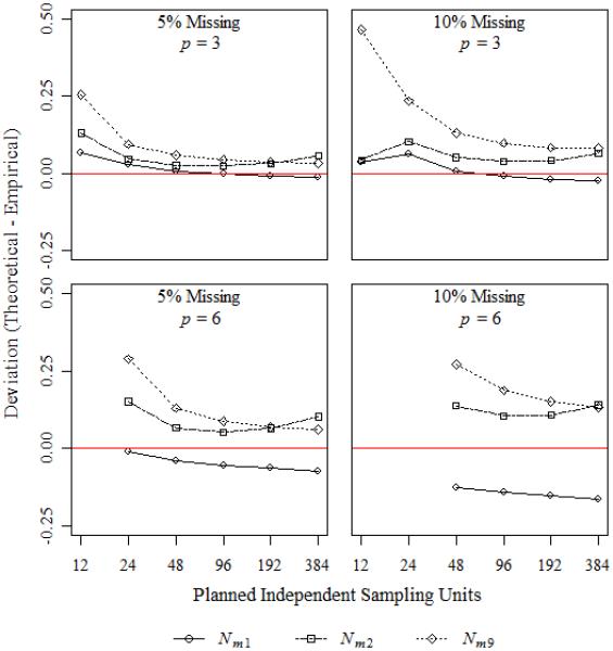
Median deviation for 90% complete data power.
Figure 2.
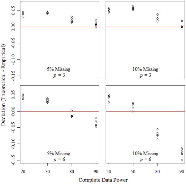
Deviations for power approximations using Nm1 and experimental designs with Nt= 48.
The accuracy of all three power approximations was largely unaffected by changes in variance structure and type of non-centrality (Table IV). However, the percentage of missing data and the number of repeated measures did affect accuracy for all three approximations. The power approximation using Nm1 retained accuracy for designs involving p = 3, no matter the percentage of missing data.
Figure 1 shows the effect of sample size on the accuracy of the three power approximations. The designs considered were all chosen so that the complete data power was 90%. For designs with p = 6, the EM algorithm converged for fewer than 10% of trials for most designs with Nt ≤ 24. Deviations were smaller for designs with fewer repeated measures and a smaller percentage of missing data. For power approximations using Nm1, deviations became smaller as sample size increased, with good performance by Nt = 48. The maximum absolute deviation for approximations using Nm1 and designs with p = 3 was 0.02, even with 10% missing data. By contrast, the power approximations using Nm2 and Nm9 overestimated the empirical power across all sample sizes. None of the power approximations performed well for p = 6, and 10% missing data.
In Figure 2, the complete data power was demonstrated to have little effect on the accuracy of the power approximation using Nm1. Here, the focus was on designs with Nt = 48. For most experimental scenarios, the power approximation using Nm1 was within approximately 0.05 of the empirical power irrespective of the complete data power. Accuracy was best for designs with fewer repeated measures and less missing data. With p = 6, and 10% missing data, the performance of the approximation was poor.
6. Demonstration
To demonstrate the utility of the method, we conduct a power analysis for a hypothetical oral cancer biomarkers study. Cancer of the head and neck has a 50% five-year survival rate and up to two times the mortality rate in black males [15]. The high mortality rate is believed to be due to late stage diagnosis and treatment [15-17]. To facilitate earlier identification of disease, Elashoff et al. [18] evaluated 10 salivary biomarkers for the detection of oral squamous cell carcinoma. The biomarkers showed increased expression in cases over normal controls.
Suppose a researcher would like to validate three of the salivary biomarkers studied by Elashoff et al. [18], IL-1B, IL-8, and SAT, in the Veterans Affairs population. The researcher plans an unmatched case/control study. There will be 75 participants with diagnosed oral squamous cell carcinoma, and 75 participants without carcinoma. A saliva sample will be taken from each participant and analyzed to determine the levels of each biomarker. The researcher wishes to test the null hypothesis that there is no difference between cases and controls in the mRNA expression levels for any biomarker.
Per the recommendations of Muller et al. [1], the researcher plans to use a general linear multivariate model (Equation 2) and the Hotelling-Lawley trace. The planned Y is a (150 × 3) matrix containing the mRNA expression levels for the three biomarkers and X = I2 ⊗ 1(150/2, 1). For power analysis, the researcher plans to use α = 0.05, C = [1 –1], U = I3, and a compound symmetric , with σ2 = 2.9 and ρ = 0.4. In addition, the researcher considers B = [μc μn]′, with control means , δ′ = [–1.3 –2.1 –1.4] and case means . The values for σ2, μc, μn, and δ are extrapolated from Table 3 in Elashoff et al. [18]. The parameter ρ is chosen arbitrarily. In a real power analysis, ρ would be based either on the literature or on the previous experience of the researcher. The constant K is used to vary the difference in group means. Note that, when K = 0, μc, = μn and there is no difference between the cases and controls on levels of the biomarkers. When K = 1, mean biomarker levels for each of the three biomarkers exactly match those of Cohort 4, in Table 3 of Elashoff et al. [18].
Table III.
Sandwich estimator Type I error rates for target α = 0.05, time by treatment test, p times, two groups, Nt independent sampling units.
| Nt | p | Type I Error |
|---|---|---|
| 10 | 4 | 0.15 |
| 10 | 8 | 0.37 |
| 40 | 4 | 0.07 |
| 40 | 8 | 0.08 |
| 40 | 32 | 0.30 |
The power analysis must account for potential missing data. Funds for the study are limited and failed assays will not be rerun, which could result in randomly missing data points. The researcher anticipates a 6% assay failure rate [19]. To account for the missing data, the researcher will use the modified F test recommended by Catellier and Muller [2].
The researcher calculates power for the study using E(Nm1), as suggested in Section 4. Power curves for 0%, 5%, and 10% missing data are shown in Figure 3. At the planned sample size, the study has 90% power for mean differences at least as great as those observed by Elashoff et al. [18] and up to 10% missing data.
Figure 3.
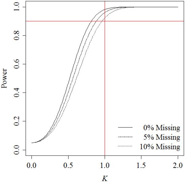
Power curves for a hypothetical oral cancer biomarkers study.
Example SAS/IML code for the oral cancer biomarker power analysis is given in Appendix D.
7. Discussion
Accurate sample size calculation is a vital component of responsible research. Overestimation of the sample size can expose study participants to unnecessary risk. Underestimation of the sample size can result in studies that cannot be replicated, and which exhaust resources that could have been used for conclusive scientific progress.
The approach presented in the current work gives a general method to approximate power for balanced linear mixed models using a multivariate test. The approach extends power methods for the balanced linear mixed model with complete data [1] to similar models with missing data. The manuscript focuses on an adjusted multivariate Hotelling-Lawley trace test [2] since that test provides accurate Type I error rate, even in small samples. It is important to develop a power method aligned with the planned data analytic approach [8].
The new power approximations can be implemented using the module and example provided in Appendices C and D, respectively. Copies of the free open-source module and example also appear at www.SampleSizeShop.org. The implementation has two steps. First, a custom SAS/IML [20] module computes the expected values of Nm1, Nm2 or Nm9, as desired. Next, the chosen expected value is passed into POWERLIB [21, Version 2.2]. POWERLIB then provides the chosen power approximation for the Hotelling-Lawley trace statistic.
The power approximations can also be computed using alternative, readily available software packages. The simple module to compute the expected values of Nm1, Nm2 or Nm9 can be ported easily to other programming languages, such as R [22] or MATLAB [23]. To compute the power, users may choose any power software that provides approximations for multivariate tests. Examples include PASS [24] or GLIMMPSE [25]. If the program does not allow use of fractional sample sizes, the user may need to round the expected values of Nm1, Nm2 or Nm9 to the nearest whole number.
We provide the following recommendations for researchers who choose to use the power approximations:
-
1)
For most experimental designs using the balanced linear mixed model, we recommend that researchers use the power approximation with Nm1 to approximate power. The approximations using Nm2 and Nm9 tend to overestimate the power. By contrast, the approximation using Nm1 is either very accurate, or provides a slight underestimation.
-
2)
In designs with large numbers of repeated measures and a high anticipated amount of missing data, all of the power approximations deviate substantially from the empirical power. Under these conditions, the choice of power approximation should balance the benefits of the research with the potential harms to study participants. In some cases, the study presents no great harm to participants. Thus, researchers may desire a liberal sample size calculation, one that will enroll more than enough participants. If so, the researchers should use the approximation with Nm1. If the study may expose participants to harm, study designers should be conservative in their approach and enroll as few participants as possible. If so, researchers should choose the approximations using Nm2 or Nm9.
-
3)
Researchers designing studies with small sample sizes and large numbers of repeated measures who expect more than 10% missing data should consider alternatives to the Catellier and Muller [2] data analysis. For many such designs, the Catellier and Muller [2] approach fails more than 9 out of 10 times. If the variance model is known, study investigators should use the Wald test with Kenward-Roger denominator degrees of freedom [4].
8. Future work
Development of approximations for power often require consideration of multiple realizations of some random factor. Random factors may include, for example, the pattern of missing data [the current work, 11, 26] or a random covariate [27-29]. In this manuscript, and in the papers on random covariates, a common approach is described to account for the random factors. The expectation of the power over all possible realizations of the random factor is approximated by the power function, evaluated at the expected value of the random factor. A similar approach should work for other problems with random factors, including random and random time- or spatially-varying covariates, or covariates that vary within groups or clusters. In addition, the approach could be applied to the Wald statistic for the mixed model with missing data.
In order to calculate the expected value of the random missing data patterns, Ringham et al. (in submission) assumed a specific probability process. In future work, additional missing data probability processes will be considered. One process of interest allows for correlation between dij and dij′. Another process of interest includes a conditional relationship between dij and di(j+1) so that, if yij is missing then yi(j+1) is also likely to be missing. This process produces monotone missing data with a high probability.
Acknowledgements
The research presented in this paper was supported by NIDCR 3R01DE020832-01A1S1, a minority supplement to NIDCR 3R01DE020832-01A1. The parent grant was awarded to the University of Florida, Keith Muller, Principal Investigator, with a subaward to the Colorado School of Public Health. Revisons to the original manuscript were supported by NCI 5R25CA087949-14, a training grant awarded to the University of California, Los Angeles, Roshan Bastani, Principal Investigator. The content of this paper is solely the responsibility of the authors, and does not necessarily represent the official views of the National Institute of Dental and Craniofacial Research, the National Cancer Institute nor the National Institutes of Health. This manuscript was submitted to the Department of Biostatistics and Informatics in the Colorado School of Public Health, University of Colorado Denver, in partial fulfillment of the requirements for the degree of Doctor of Philosophy in Biostatistics for B. M. Ringham.
Appendix A
Table V reproduces results from Ringham et al. (in submission). Using the results in the table, estimate E(Nm2) as:
Appendix B
The numerical evaluations in the current work used variances and correlations as in Barton and Cramer [12] and Catellier and Muller [2], reproduced below. Write σ2(p, v), v ∈ {Equal, Unequal} to specify the vector of variances used for p repeated measures and i type of variance. Similarly, let ρ(p, w), w ∈ {Low, High} indicate the correlation matrix used for p repeated measures and w type of correlation. Define
and
Appendix C
The following SAS/IML module computes the expected value of Nm1, Nm2, or Nm9 An example call is listed in the “Usage” line of the header comment.


Appendix D
The SAS/IML program below uses the power approximation with E(Nm1) to calculate power for the oral cancer biomarkers example in Section 6. Inputs for the power analysis are taken from Table 3 in Elashoff et al. [18]. The program uses the NMK module in Appendix C to compute E(Nm1). The expectation is passed into POWERLIB, which approximates power for the multivariate hypothesis tests using E(Nm1) as an adjusted sample size. Power in approximated for a range of effect sizes and percentages of missing data. Results are output as a power curve (Figure 3, Section 6).
Note that, should the user wish to approximate power with an alternate statistical package, the program could be truncated prior to the POWERLIB call. Results from the NMK module could be output to a dataset. The dataset could then be imported into a statistical package of the user's choice.


References
- 1.Muller KE, Edwards LJ, Simpson SL, Taylor DJ. Statistical tests with accurate size and power for balanced linear mixed models. Statistics in Medicine. 2007;26(19):3639–3660. doi: 10.1002/sim.2827. DOI: 10.1002/sim.2827. [DOI] [PubMed] [Google Scholar]
- 2.Catellier DJ, Muller KE. Tests for Gaussian repeated measures with missing data in small samples. Statistics in Medicine. 2000;19(8):1101–1114. doi: 10.1002/(sici)1097-0258(20000430)19:8<1101::aid-sim415>3.0.co;2-h. [DOI] [PubMed] [Google Scholar]
- 3.Little RJA, Rubin DB. Statistical Analysis with Missing Data. 2nd ed. Wiley-Interscience; Hoboken, New Jersey, USA: 2002. [Google Scholar]
- 4.Kenward MG, Roger JH. Small sample inference for fixed effects from restricted maximum likelihood. Biometrics. 1997;53(3):983–997. DOI: 10.2307/2533558. [PubMed] [Google Scholar]
- 5.Fouladi RT, Shieh Y-Y. A comparison of two general approaches to mixed model longitudinal analyses under small sample size conditions. Communications in Statistics-Simulation and Computation. 2004;33(3):807–824. DOI:10.1081/SAC-200033260. [Google Scholar]
- 6.Serrano D. Error of Estimation and Sample Size in the Linear Mixed Model. ProQuest, UMI Dissertation Publishing; Ann Arbor, Michigan, USA: 2008. [Google Scholar]
- 7.Gurka MJ, Edwards LJ, Muller KE. Avoiding bias in mixed model inference for fixed effects. Statistics in Medicine. 2011;30(22):2696–2707. doi: 10.1002/sim.4293. DOI: 10.1002/sim.4293. [DOI] [PMC free article] [PubMed] [Google Scholar]
- 8.Muller KE, Lavange LM, Ramey SL, Ramey CT. Power calculations for general linear multivariate models including repeated measures applications. Journal of the American Statistical Association. 1992;87(420):1209–1226. doi: 10.1080/01621459.1992.10476281. [DOI] [PMC free article] [PubMed] [Google Scholar]
- 9.Muller KE, Stewart PW. Linear Model Theory: Univariate, Multivariate, and Mixed Models. 1st ed. Wiley-Interscience; Hoboken, New Jersey, USA: 2006. [Google Scholar]
- 10.McKeon JJ. F Approximations to the distribution of Hotelling's T02. Biometrika. 1974;61(2):381–383. [Google Scholar]
- 11.Tu XM, Zhang J, Kowalski J, Shults J, Feng C, Sun W, Tang W. Power analyses for longitudinal study designs with missing data. Statistics in Medicine. 2007;26(15):2958–2981. doi: 10.1002/sim.2773. DOI: 10.1002/sim.2773. [DOI] [PubMed] [Google Scholar]
- 12.Barton CN, Cramer EC. Hypothesis testing in multivariate linear models with randomly missing data. Communications in Statistics - Simulation and Computation. 1989;18(3):875–895. DOI: 10.1080/03610918908812796. [Google Scholar]
- 13.Olson CL. Comparative robustness of six tests in multivariate analysis of variance. Journal of the American Statistical Association. 1974;(348):894–908. 69. DOI:10.1080/01621459.1974.10480224. [Google Scholar]
- 14.Dempster AP, Laird NM, Rubin DB. Maximum likelihood from incomplete data via the EM algorithm. Journal of the Royal Statistical Society, Series B. 1977;39(1):1–38. [Google Scholar]
- 15.Shiboski CH, Schmidt BL, Jordan RCK. Racial disparity in stage at diagnosis and survival among adults with oral cancer in the US. Community Dentistry and Oral Epidemiology. 2007;35(3):233–240. doi: 10.1111/j.0301-5661.2007.00334.x. DOI: 10.1111/j.0301-5661.2007.00334.x. [DOI] [PubMed] [Google Scholar]
- 16.Mashberg A, Samit AM. Early detection, diagnosis, and management of oral and oropharyngeal cancer. CA: A Cancer Journal for Clinicians. 1989;39(2):67–88. doi: 10.3322/canjclin.39.2.67. [DOI] [PubMed] [Google Scholar]
- 17.Peacock ZS, Pogrel MA, Schmidt BL. Exploring the reasons for delay in treatment of oral cancer. Journal of the American Dental Association. 2008;139(10):1346–1352. doi: 10.14219/jada.archive.2008.0046. [DOI] [PubMed] [Google Scholar]
- 18.Elashoff D, Zhou H, Reiss J, Wang J, Xiao H, Henson B, et al. Prevalidation of salivary biomarkers for oral cancer detection. Cancer Epidemiology, Biomarkers & Prevention. 2012;21(4):664–672. doi: 10.1158/1055-9965.EPI-11-1093. DOI:10.1158/1055-9965.EPI-11-1093. [DOI] [PMC free article] [PubMed] [Google Scholar]
- 19.Andreson R, Möls T, Remm M. Predicting failure rate of PCR in large genomes. Nucleic Acids Research. 2008;36(11):e66. doi: 10.1093/nar/gkn290. DOI: 10.1093/nar/gkn290. [DOI] [PMC free article] [PubMed] [Google Scholar]
- 20.SAS Institute Inc. SAS/IML® 9.22 User's Guide. SAS Institute Inc; Cary, North Carolina, USA: 2010. [Google Scholar]
- 21.Johnson JL, Muller KE, Slaughter JC, Gurka MJ, Gribbin MJ, Simpson SL. POWERLIB: SAS/IML software for computing power in multivariate linear models. Journal of Statistical Software. 2009;30(5):1–27. doi: 10.18637/jss.v030.i05. [DOI] [PMC free article] [PubMed] [Google Scholar]
- 22.R Development Core Team . R: A Language and Environment for Statistical Computing. R Foundation for Statistical Computing; Vienna, Austria: 2011. [Google Scholar]
- 23.MATLAB and Statistics Toolbox. The MathWorks, Inc; Natick, Massachusetts, USA: 2012. URL http://www.mathworks.com. [Google Scholar]
- 24.NCSS . LLC (NCSS Statistical Software) PASS; Kaysville, Utah, USA: 2001. URL http://www.ncss.com. [Google Scholar]
- 25.Kreidler SM, Muller KE, Grunwald GK, Ringham BM, Coker-Dukowitz ZT, Sakhadeo UR, Barón AE, Glueck DH. GLIMMPSE: Online power computation for linear models with and without a baseline covariate. Journal of Statistical Software. 2013;54(10):i10. doi: 10.18637/jss.v054.i10. URL http://www.glimmpse.org. DOI: 10.18637/jss.v054.i10. [DOI] [PMC free article] [PubMed] [Google Scholar]
- 26.Verbeke G, Lesaffre E. The effect of drop-out on the efficiency of longitudinal experiments. Journal of the Royal Statistical Society, Series C. 1999;48(3):363–375. DOI: 10.1111/1467-9876.00158. [Google Scholar]
- 27.Sampson AR. A tale of two regressions. Journal of the American Statistical Association. 1974;69(347):682–689. DOI:10.1080/01621459.1974.10480189. [Google Scholar]
- 28.Gatsonis C, Sampson AR. Multiple correlation: Exact power and sample size calculations. Psychological Bulletin. 1989;106(3):516–524. doi: 10.1037/0033-2909.106.3.516. [DOI] [PubMed] [Google Scholar]
- 29.Glueck DH, Muller KE. Adjusting power for a baseline covariate in linear models. Statistics in Medicine. 2003;22(16):2535–2551. doi: 10.1002/sim.1341. DOI: 10.1002/sim.1341. [DOI] [PMC free article] [PubMed] [Google Scholar]