Simultaneous Denoising, Deconvolution, and Demixing of Calcium Imaging Data

SUMMARY

We present a modular approach for analyzing calcium imaging recordings of large neuronal ensembles. Our goal is to simultaneously identify the locations of the neurons, demix spatially overlapping components, and denoise and deconvolve the spiking activity from the slow dynamics of the calcium indicator. Our approach relies on a constrained nonnegative matrix factorization that expresses the spatiotemporal fluorescence activity as the product of a spatial matrix that encodes the spatial footprint of each neuron in the optical field and a temporal matrix that characterizes the calcium concentration of each neuron over time. This framework is combined with a novel constrained deconvolution approach that extracts estimates of neural activity from fluorescence traces, to create a spatiotemporal processing algorithm that requires minimal parameter tuning. We demonstrate the general applicability of our method by applying it to in vitro and in vivo multineuronal imaging data, whole-brain light-sheet imaging data, and dendritic imaging data.

INTRODUCTION

Calcium imaging is becoming a standard tool for monitoring large neuron populations. Recent technical advances have enabled complete imaging of small cortical volumes (e.g., Cotton et al., 2013), and whole-brain imaging of small animals (Ahrens et al., 2013; Prevedel et al., 2014) at reasonable imaging rates. In parallel, engineering of genetically encoded calcium indicators offers increasingly sensitive indicators that can reliably detect action potentials in vivo (Chen et al., 2013). From a statistical perspective, these developments pose significant challenges, which can be condensed to three major problems: (1) identifying the spatial footprint of each neuron in the optical field, (2) demixing spatially overlapping neurons (where overlap is due either to the projection of a 3D volume onto a 2D imaging plane or to insufficient spatial resolution in 3D imaging methods), and (3) deconvolving the spiking activity of each neuron from the much slower dynamics of the calcium indicator. These tasks become harder due to the existence of measurement noise, unaccounted neural processes and/or neuropil activity, and limitations in imaging rate.

Traditionally, these three problems have been dealt with separately. Calcium deconvolution methods have focused largely on analyzing one-dimensional fluorescence time series data from one neuron at a time. Such methods include fast nonnegative deconvolution (Vogelstein et al., 2010), greedy algorithms (Grewe et al., 2010), finite rate of innovation methods (Oñativia et al., 2013), supervised learning (Theis et al., 2015), as well as particle filtering (Vogelstein et al., 2009) and Markov chain Monte Carlo (MCMC) methods (Pnevmatikakis et al., 2013). Although effective in the analysis of single fluorescence traces, these methods do not take full advantage of the spatiotemporal structure in the data, and in some cases require either data with available ground truth and/or significant parameter tuning.

Solutions to the spatial location identification problem are usually based on two observations: first, neurons are often spatially localized, yielding methods based on local correlations of neighboring pixels (Smith and Häusser, 2010), dictionary learning (Pachitariu et al., 2013), or graph-cut-related algorithms (Kaifosh et al., 2014). These methods typically aggregate the activity over time to produce a summary statistic (e.g., the mean, maximum, or correlation image or a weighted graph representation between the different imaged pixels) that is then processed (e.g., segmented) to identify the spatial components. While these methods can yield localized estimates, they do not account explicitly for the calcium dynamics, and more importantly their performance can deteriorate in the case of significant spatial overlap, since an aggregated summary image (e.g., the mean) will not be able to distinguish between different overlapping neurons.

A second approach stems from the observation that spatiotemporal calcium activity can be approximated as a product of two matrices: a spatial matrix that encodes the location of each neuron in the optical field, and a temporal matrix that characterizes the calcium concentration evolution of each neuron. Based on this observation Mukamel et al. (2009) proposed an Independent Component Analysis (ICA) approach that seeks spatiotemporal components that have reduced dependence. While simple and widely used in practice, ICA is an inherently linear demixing method and can fail in practice when no linear demixing matrix is available to produce independent outputs, as is often the case when the neural components exhibit significant spatial overlap.

To overcome this problem, two nonlinear matrix factorization methods have been proposed: multilevel sparse matrix factorization (Diego-Andilla and Hamprecht, 2013) and nonnegative matrix factorization (NMF) (Maruyama et al., 2014). These methods can deal more effectively with overlapping neural sources but do not explicitly model the calcium indicator dynamics and do not always provide compact spatial footprint estimates. In this paper, we approach the factorization, deconvolution, and denoising problems simultaneously, by introducing a constrained matrix factorization method that decomposes the spatiotemporal activity into spatial components with local structure and temporal components that model the dynamics of the calcium. By accounting for overlapping neuronal spatial footprints, we can obtain improved temporal deconvolution results, and conversely by imposing a structured model of the dynamics of the calcium indicator, we can obtain improved identification of the spatial footprints of the observed neurons, especially in low signal-to-noise ratio (SNR) areas.

A key characteristic of our approach is that it requires no tuning of regularization parameters that control the tradeoff between the fidelity to the data and some desired signal structure (e.g., sparsity), as is necessary in related methods that have appeared recently in the literature (Pnevmatikakis and Paninski 2013; Haeffele et al., 2014; Diego-Andilla and Hamprecht, 2014). Instead, we take a constrained deconvolution (CD) approach, in which we seek the sparsest neural activity signal that can explain the observed fluorescence up to an estimated measurement noise level. We then embed this CD approach within a constrained nonnegative matrix factorization (CNMF) framework that enforces the dynamics of the calcium indicator and automatically sets individual sparsity constraints for both the spiking activity and the shape of each inferred neuron.

We first apply our deconvolution and denoising methods to time series calcium imaging datasets for which ground truth is available. Such datasets are important for quantitatively assessing the performance of deconvolution algorithms, but in practice are typically not available, emphasizing the need for unsupervised methods like those described here. Next, we apply our CNMF framework to analyze a variety of large scale in vitro and in vivo datasets. The results indicate that our framework can handle different types of imaging data in terms of imaged brain location, frame rate, imaging technology, and imaging scale, in a flexible and computationally efficient way that requires minimal human intervention. A further example is provided in the companion paper (Yang et al., 2015), where our new analysis methods help enable a novel multi-plane imaging technique. We discuss the results of these various analyses next, deferring all technical methodological details to the Experimental Procedures and the Supplemental Experimental Procedures.

RESULTS

Constrained Sparse Nonnegative Calcium Deconvolution

We first address the problem of deconvolving the neural activity from a time series trace of recorded fluorescence. In principle, this is achievable when the imaging rate is fast, i.e., the time between two consecutive measurements is small compared to the calcium indicator decay time constant. Modern resonant scanning (Rochefort et al., 2009), random access microscopy (Duemani Reddy et al., 2008), and scanless imaging (Nikolenko et al., 2008) protocols can allow for this, by recording neural ensembles at high rates. Under this regime, we take a completely unsupervised approach for performing deconvolution that can be summarized as follows: first, we estimate a parametric model for the calcium concentration transient response that would be evoked by a single spike. Instead of fitting a parametric model to isolated calcium transients evoked by single spikes (often only available from dual electrophysiological recording and imaging experiments, as in e.g., Grewe et al. [2010]), we approximate the calcium transient as the impulse response of an autoregressive (AR) process of order p (with p small, just 1 or 2 in all the examples presented here), which models the rise and decay time constants; this AR(p) model is estimated by adapting standard AR estimation methods. After determining the shape of the calcium transient, we estimate the spiking signal by solving a non-negative, sparse constrained deconvolution (CD) problem: we seek the sparsest nonnegative neural activity signal that fits the data up to a desired noise level, which is estimated from the power spectral density of the observed fluorescence trace. The resulting optimization problem is convex, i.e., it has no local minima, and can be solved efficiently, with complexity that scales just linearly with the number of observed timesteps, and quadratically with the (modest) AR order p, and not with the length of the transient response; see Experimental Procedures and the Supplemental Experimental Procedures for full details.

While the AR parameter identification process is often very useful in estimating the transient response that would arise from a single spike, it is useful to refine these estimates given initial estimates of the spike times. We found that an extension of the Markov Chain Monte Carlo (MCMC) methods described in Pnevmatikakis et al. (2013) provided an effective strategy (see the Supplemental Experimental Procedures for full details).

We tested these methods using an in vitro dataset of n = 207 spinal motor neurons obtained from seven sequentially acquired imaging fields in a single preparation (Figure 1). The neurons expressed the GCaMP6s indicator and were stimulated under an antidromic stimulation protocol that caused them to reliably fire in patterns that matched the stimulus pulses (similar to Machado et al., 2015); we treat the antidromic stimulus spike times as ground truth in this setting, though this neglects the effect of spontaneous (non-antidromically driven) activity on the observed fluorescence data. The imaging rate was 14.6 Hz and a first-order AR model (p = 1) was found to be sufficient to model the calcium dynamics in this case. To quantify the performance, we computed the correlation between the true spiking signal (as is defined by the stimulus timing) and the inferred spiking signal, binned at the resolution defined by the imaging rate or coarser.

Figure 1. Application of the CD Method to Antidromically Driven In Vitro Spinal Cord Data.

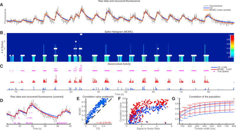
(A) Raw fluorescence data from an example neuron (gray) and reconstructed fluorescence trace with the proposed CD method (blue) and the mean sample obtained by the fully Bayesian MCMC method of Pnevmatikakis et al. (2013), with time constant updating (red). The CD method effectively denoises the observed fluorescence trace but overestimates the time constants slightly, while the more expensive MCMC method fine-tunes the time constants to match better the observed data.

(B) Color-coded depiction of the empirical posterior marginal histogram obtained with the MCMC method and true number of antidromic spikes during each timebin (white dots). The colormap displays the probability of a certain number of spikes within a given timebin. The MCMC method can quantify uncertainty and identify multiple spikes within a single timebin.

(C) Estimated neural activity (normalized) from the CD method (blue) and mean of the posterior marginal per timebin with the MCMC method (red). The legend also shows the spike correlation for each method at the imaged resolution. All methods detect accurately the bursting intervals of the neurons. The more expensive MCMC method gives a significant improvement in the spike deconvolution according to the spike correlation metric.

(D) Zoomed-in version of (A).

(E) MCMC outperforms CD for this dataset (Wilcoxon signed ranked test). Each circle corresponds to a single cell.

(F) Correlation values at the imaged resolution for all n = 207 cells as a function of the signal-to-noise ratio for the two methods. Performance increases with the SNR for all methods. Again, each circle corresponds to a single cell.

(G) Median correlation values for all n = 207 cells at various timebin widths. Error bars indicate the 0.25 and 0.75 quantiles, respectively.

Figure 1A shows the reconstructed calcium trace for the CD algorithm (blue), and the mean calcium trace obtained with 500 samples from the MCMC algorithm (red) superimposed on the raw data (gray), and indicates that both methods track the observed fluorescence trace fairly well; however, the MCMC method can modify the inferred time constants to better fit the data (Figure 1A). Note that the MCMC method here was initialized with the results obtained with the CD approach. The MCMC method produces samples of spike trains with continuous time resolution, and thus it can provide further insight into the number of spikes produced at every timebin and the uncertainty of these estimates due to noise and finite imaging rate. This is shown in panel B, where the marginal posterior of the number of spikes at each timebin is plotted and the true number of spikes (or stimulations) in this case is also shown (purple dots). This temporal uncertainty quantification is not available with the CD algorithm, which is based on a convex optimization framework and thus provides just a single estimate of the neural activity, binned at the imaging rate resolution. Panel C shows the inferred spiking signals for both methods and panel D displays the recovered traces and true antidromic stimulus spikes in more detail in a zoomed-in temporal interval. A comparison of the two methods for the whole population of the 207 neurons is shown in Figures 1E–1G. The computationally more intensive MCMC approach outperforms the CD method for almost every cell (Wilcoxon signed rank test). The achieved correlation values increase, on average, with SNR (Figure 1F; SNR computed as the ratio between the standard deviation (SD) of the inferred calcium trace and the SD of the noise, as inferred from the MCMC method). Both inference methods improve their correlation coefficient at more coarse resolutions (Figure 1G). In the Supplemental Information (Figure S1), we apply these methods to a different publicly available dataset with ground truth, where the imaging rate is much higher (60 Hz) and AR(2) methods improve the deconvolution results significantly. We also illustrate the parameter identification and time constant updating methods in greater detail.

The proposed AR framework makes a number of simplifying assumptions on the fluorescence dynamics, with the benefit of increased computational tractability. The dynamics are assumed to be linear and time invariant, and no saturation level is assumed. It is possible to find clear violations of these assumptions in Figure 1A: bursts of spiking activity at the beginning of the trial, e.g., in the interval [10,20]s, have a weaker effect than bursts toward the end of the trial, and the strong bursts in the zoomed interval displayed in Figure 1D do not appear to add up linearly. It is natural to ask how much the performance of the algorithm might be limited by these unmodeled nonlinearities. Machado et al. (Machado et al., 2015, their Figure S1) addressed this question using data nearly identical to that used here (but with a different calcium indicator), by including an additional sigmoidal nonlinearity. Although this approach does not model the biophysical properties of the indicator binding, it can still be helpful in capturing weak activation from single spikes and saturation effects. The analysis in that paper showed that there was no statistically significant difference in the performance of the CD algorithm when this nonlinearity was included. Similar results were obtained here for the data shown in Figure 1 (Wilcoxon signed ranked test, p value 0.65, data not shown). Thus, in the following we use the simple linear AR model as the building block for our spatiotemporal framework but note that the choice of temporal deconvolution method is largely independent of the spatiotemporal demixing methods presented next; therefore, as discussed in the Experimental Procedures, other deconvolution methods that incorporate nonlinear effects (such as the particle filter methods discussed in Vogelstein et al., 2009) could easily be integrated within the framework presented here.

A Constrained Nonnegative Matrix Factorization Approach for the Analysis of Spatiotemporal Calcium Imaging Data

The problem of identifying the spatial footprint of each imaged neuron is also known in the literature as a problem of region of interest (ROI) selection or image segmentation. While these terms are intuitive, we prefer to use the phrase “spatial footprint identification,” which does not preclude significant overlap between the footprints of different neurons. In contrast, in (manual) ROI selection, a compact set of pixels/voxels is typically assigned to each neuron and the signal is then obtained by averaging the spatial ROI. Similarly, in image segmentation techniques, each pixel/voxel is generally assigned to a different object and overlap is not allowed. Here we argue that preventing spatial overlap during spatial footprint identification can potentially lead to significant levels of “cross-talk” between spatially overlapping components, lower SNR, and therefore to misleading results; further examples are provided in the companion paper (Yang et al., 2015).

We approach this problem by employing a CNMF framework that decomposes the data into a spatial matrix that encodes the spatial footprint of each neuron and a temporal matrix that encodes the time-varying calcium activity of each neuron, together with components that model the background/neuropil activity. This procedure denoises the spatiotemporal fluorescence up to a desired voxel-dependent noise level and infers compact neuron shapes with fluorescence dynamics that obey the dynamics of the calcium indicator. We also include methods for merging spatial components that correspond to the same neuron, by combining components that overlap spatially and are significantly correlated temporally, and methods for removing components that do not correspond to neurons and/or have insignificant temporal contributions. We assume that all the data has been pre-processed to correct for motion artifacts during acquisition, although the proposed methods can tolerate small motion artifacts compared to the size of the spatial components. Moreover, our methods can handle missing data, e.g., due to motion in line-scanned methods. In the Experimental Procedures and the Supplemental Experimental Procedures, we present more details about the iterative algorithms we use to compute the matrix factorization solution (in which we first optimize with respect to the temporal components with the spatial footprints held fixed, then vice versa); the resulting solutions can be computed efficiently and in many cases are readily parallelizable.

The problem of optimally decomposing a matrix into a product of two other matrices is not convex, and alternating minimization methods such as those developed here converge only to a local optimum, which depends on the initial starting point. In some cases, good initializations are available: for example, through dual labeling of neurons so that the nucleus is labeled with a non-fluctuating red signal, while calcium imaging in the soma is performed in the green channel. Our core framework could be initialized by segmenting the red channel, or more broadly by any method that provides useful information about the locations of the observed neurons. When no initialization is already available, we designed two initialization algorithms effective in the case of somatic imaging. The first is an efficient greedy method that searches for a user-specified number of compact spatial regions that explain a significant percent of the variance observed in the data. The second is a convex approach that uses Gaussian spatial filtering to group correlated neighboring pixels together and initialize the spatial locations, while at the same time controlling for the number of formed groups via a “group lasso” (GL) penalty. We focus on applications of this procedure in the following and again defer to the Experimental Procedures and the Supplemental Experimental Procedures for a detailed presentation.

Resolving Overlapping Locations through CNMF

Before applying our CNMF framework to large-scale datasets, we illustrate through examples on artificial data its ability to demix overlapping neurons. We first constructed two largely overlapping neurons (contour plots shown in white in Figure 2A) that fired spikes according to independent Poisson processes. Due to the high degree of spatial overlap, time-aggregated measures of activity (e.g., the mean image) cannot display the existence of more than one neuron. This is illustrated again in Figure 2A, where the “correlation image” is shown. The correlation image for each pixel is computed by averaging the correlation coefficients (taken over time) of each pixel with its four immediate neighbors.

Figure 2. Resolving Overlapping Spatial Footprints in Simulated Data.

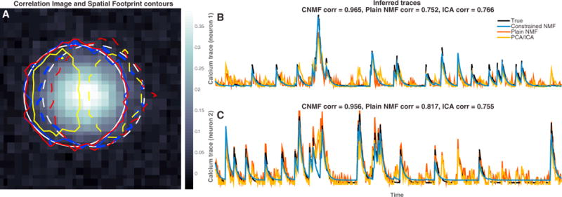
Simulated fluorescence traces were generated from two significantly overlapping neuron spatial footprints in low SNR conditions. (Both spatial and temporal units in this example are arbitrary.)

(A) Correlation image generated from the raw data and superimposed contour plots (solid for neuron 1 and dashed for neuron 2) for the true spatial footprints (white) and the inferred spatial footprints with our proposed CNMF method (blue), the plain NMF method of Maruyama et al., (2014) (red), and the PCA/ICA method of Mukamel et al., (2009) (yellow). The correlation image cannot distinguish between the two different neurons. The spatial footprints inferred by PCA/ICA are significantly smaller than the true spatial footprints. NMF methods capture the full spatial extent of the spatial footprints.

(B and C) Inferred calcium traces with all the methods. PCA/ICA and plain NMF cannot satisfactorily demix the traces and attributes single neuron activity to both neurons. On the contrary, our CNMF approach eliminates most of the “cross-talk” between the overlapping neurons. Correlation values are computed on the estimated deconvolved neural activity.

We compare our method against the popular PCA/ICA method of Mukamel et al. (2009) and the plain NMF method proposed in Maruyama et al. (2014). The PCA/ICA method searches for a matrix of linear spatial filters such that, when these filters are applied to the video data, the output time series are as independent as possible. However, in the case of significant spatial overlap, there is no such linear demixing matrix that can lead to independent outputs, and therefore in this example the PCA/ICA method tends to infer non-overlapping spatial filters (yellow contour plots in Figure 2A) by assigning pixels that should belong to both neurons to only one of the neurons and simply neglecting many pixels with strong contributions from both neurons. This solution has two shortcomings. First, since some overlapping pixels are uniquely assigned to one neuron, the inferred traces exhibit significant amounts of “cross-talk” (yellow traces in Figures 2B and 2C) that is potentially misleading for understanding the spiking activity of each neuron. (This cross-talk would corrupt any analysis that depends on the cross-correlation between these two neurons, for example.) Second, by excluding many overlapping high-SNR pixels, the temporal traces are computed over a smaller spatial region, resulting in decreased total output SNR. (See the companion paper, Yang et al. [2015], for further examples and analysis of this effect in real data.) The NMF method proposed in Maruyama et al. (2014) is a nonlinear demixing method and can therefore better handle spatially overlapping signals, especially in high-SNR conditions. However, this method (as well as PCA/ICA) does not model the temporal dynamics of the calcium indicator or impose any sparsity or locality constraints and thus can produce very noisy output traces (Figures 2B–2C, red traces), reducing the effective SNR of the output signals and again allowing for “cross-talk.”

In contrast, the CNMF method infers the spatial footprints of the two neurons very accurately (blue contour plots in Figure 2A) and demixes their activity over time with almost zero “cross-talk” between the two traces and minimal noise (blue traces in Figures 2B and 2C). More technical information about this example can be found in the Supplemental Experimental Procedures.

We next examined the robustness of these methods as a function of the measurement noise level. We constructed a population of ten partially overlapping neurons placed randomly in a field of view (an example is shown in Figures 3A–3C), against a uniformly time-varying background. These neurons again fired spikes according to independent Poisson processes. We then simulated Gaussian white noise for each pixel, with SD proportional to the mean activity at this pixel, resulting in an approximately uniform SNR across the whole field of view. A range of different noise levels was considered, spanning over an order of magnitude of SNR. We repeated each simulation five times and considered two different neuron shapes that are encountered in practice: (1) “donut”- (as seen in panels A–C, corresponding to expression at the cytosolic regions of the cells and excluding the nucleus) and (2) “Gaussian”-shaped neurons (more similar to the simulated neurons shown in Figure 2). Full simulation details can be found in the Supplemental Experimental Procedures.

Figure 3. Performance of Proposed Spatiotemporal Method in Simulated Data.

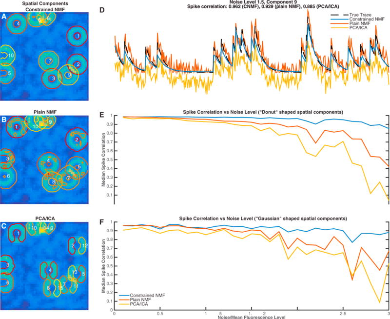
Simulated fluorescence traces were generated from a population of ten neurons placed randomly in the field of view, allowing significant spatial overlap. Two different neuronal shapes were considered across thirty different noise levels.

(A–C) Inferred spatial components with the proposed CNMF method (A), plain NMF as proposed in Maruyama et al. (2014) (B), and the PCA/ICA method of Mukamel et al. (2009) (C). Contour plots of the inferred spatial components are super-imposed on the image of mean activity. In this example, the noise level for every pixel was 1.5× the mean activity. The numbers in white are placed on the center of mass of each component. The proposed method identifies spatial components very accurately, compared to plain NMF that can group different components together. PCA/ICA tends to infer smaller non-overlapping components and can also split components into multiple parts in low SNR conditions.

(D) Inferred temporal traces for component 9 (as indicated in A). The proposed method infers a trace (blue) that matches the true trace (dashed black) much better than the plain NMF method (red) and PCA/ICA (yellow).

(E) Median spike correlation of the three methods over 30 different noise levels, with five iterations for each level, for donut-shaped neurons.

(F) Same, but for “Gaussian” shaped neurons. The proposed method is significantly more robust compared to other popular methods, especially for low-SNR conditions.

A specific instance of this simulation is shown in Figures 3A–3D, where the noise level was chosen to be 1.5× the mean activity over time. Results are similar to those shown in the previous figure; the PCA/ICA method tends to infer non-overlapping spatial filters (e.g., components 11 and 5 in Figure 3C). Moreover, in low-SNR conditions, as the example shown in Figure 3, individual neurons are sometimes mistakenly split into two components, e.g., components 2 and 12 in Figure 3C.

The plain NMF method infers the spatial components better than PCA/ICA but does not penalize for the sparsity of the spatial footprints and therefore can infer components that are not localized or combine multiple neurons that do not necessarily overlap (Figure 3B). Moreover, this method is prone to local optima in low-SNR data and requires significant manual intervention (for component selection and merging) when applied to fields of view containing many neurons. Finally, as also shown in Figure 3D, the absence of a model for the temporal dynamics of the underlying calcium signal results in noisy traces that hinder activity deconvolution.

In contrast, by (1) penalizing the size of the spatial footprints, (2) estimating the noise level of the data for each pixel, (3) modeling the indicator dynamics, and (4) using appropriate initialization methods, the CNMF method infers the spatial footprints of all the neurons very accurately (contour plots in Figure 3A) and demixes their activity over time with almost zero “cross-talk” between neighboring traces and minimal noise (blue trace in Figure 3D), with no manual intervention. Our approach remains robust even in very low-SNR conditions, where the other two methods break down (Figures 3E and 3F). These qualitative differences between the three compared methods are summarized in Table 1.

Table 1.

Qualitative Differences between the Proposed CNMF Method, PCA/ICA, and Plain NMF

Method	PCA/ICAa	Plain NMFb	Constrained NMFc
Features
Handles spatial overlap well	No	Yes	Yes
Eliminates “cross-talk”	No	Medium	Yes
Robustness in low SNR	Medium	Medium	Yes
Produces localized estimates	Yes	No	Yes
Unsupervised (after initial parameter setting)	Yes	No	Yes
Deconvolves neural activity	No	No	Yes
Models background activity	No	Yes	Yes
Enables merging	No	Manual	Automated

^aMukamel et al. (2009).

^bMaruyama et al. (2014).

^cThis paper.

Analysis of Large-Scale Imaging Data

We now turn to the analysis of large-scale spatiotemporal datasets. We begin by applying our methods to in vivo mouse V1 GCaMP6s spontaneous activity data (Figure 4). The algorithm was initialized with the greedy method (see Experimental Procedures) with 300 components. During the factorization iterations, 31 components were eliminated due to merging operations or negligible total contribution. The remaining components were ranked in decreasing order based on their size and maximum temporal value (see Experimental Procedures). The contours of the first 200 inferred spatial footprints are depicted in Figure 4A, superimposed on the correlation image of the raw data. Localized regions in the correlation image with high intensity correspond to strongly active cells, whereas localized regions with lower intensity correspond to neurons with lower intensity/SNR or other non-stationary processes. The algorithm efficiently identifies neurons with very few visually apparent false positives and denoises the calcium activity of each cell (Figure 4B). The inferred temporal traces match the time course and dynamics of the raw data. This is shown in Figure 4C, which zooms in to a point of local maximum activation for each trace (point marked in Figure 4B) and plots the traces in higher resolution superimposed with the spatial component weighted average of the raw data, after the removal of all the other components. The spatial footprints of the first 36 inferred components are shown in Figure 4D; in many cases detailed morphological structure is automatically extracted by the algorithm. The results are viewed best in Movie S1. Figure 4E displays an example of the merging procedure. The neuron depicted in the fourth panel is initially split across three components. Since the temporal activity of these components is highly correlated, they are merged into a single cell. Full implementation details are given in the Supplemental Experimental Procedures.

Figure 4. Application to Mouse In Vivo GCaMP6s Data.

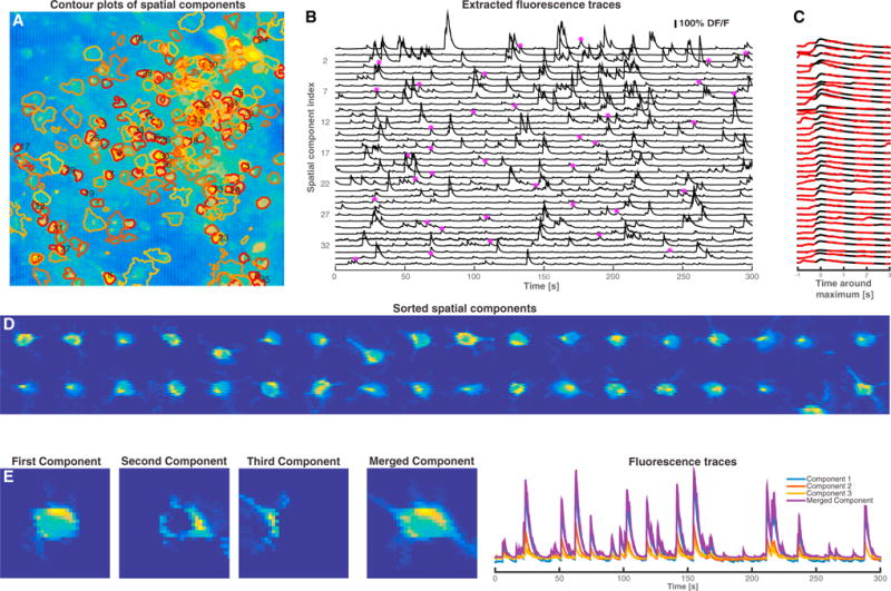
(A) Contour plots of inferred spatial components superimposed on the correlation image of the raw data. The components are sorted in decreasing order based on the maximum temporal value and their size. Contour plots of the first 200 identified components are shown, and the first 36 components are numbered.

(B) Extracted DF/F fluorescence traces for the first 36 components.

(C) Zoomed-in depiction of the fluorescence traces around a point of local maximum activity indicated by the star marker in (B), (black) super-imposed with the raw spatial component filtered data after removal of all the other components (red dashed).

(D) Spatial footprints of the first 36 components. The algorithm can in many cases pull out morphological details of the imaged processes.

(E) Depiction of the merging procedure: the first three panels in the left show three overlapping components with highly correlated temporal activity. These components are merged into a single component that is further refined in the algorithm. The temporal traces of the three initial components and the merged component are shown in the right panel (see also Movie S1).

Segmentation of Whole-Brain Light Sheet Imaging Data

Next, we test our method on a larger scale. Specifically, we examine 3D imaging data from a whole zebrafish brain (Freeman et al., 2014). The imaging was done using light-sheet microscopy, with a GCaMP6s indicator, localized to the nucleus. In this dataset, the neurons are closely packed together and sometimes exhibit highly synchronous activity. We use the group lasso (GL) approach to initialize the estimates, followed by fine-tuning using CNMF. The length of the imaging timebin (~475 ms) is comparable to the decay time constant of the calcium indicator, and the temporal details of the spiking activity cannot be estimated at a fine temporal resolution here. However, we can still utilize a similar matrix factorization framework by dropping the temporal constraints due to the calcium dynamics and then inferring the spatial and temporal components.

The resulting spatial and temporal components are shown in Figures 5A and 5B. These generally match the neuronal shapes and the sparse nature of the activity visible in the Movies S2, S3, and S4. Specifically, high-ranking spatial components usually have smoother, more consistent spheroid shapes (consistent with the nuclear-localized calcium indicator) and the corresponding temporal components tend to be sparser. Low-ranking shapes seem to correspond to faint or partially obstructed neurons. In total, the algorithm detects a realistic distribution of components throughout the brain (Movie S8). Most visible neurons are detected, as can be seen in Figures 6A, 6C, and 6E, and more clearly in the Movies S2, S3, and S4.

Figure 5. Components Detected in a Whole Zebrafish Brain.

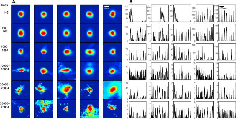
A sample of detected components (A, inferred neuronal shapes; B, inferred DF/F activity traces), ordered according to their rank. High-ranking components match expected nuclear-localized neuronal shapes and activity visible in the raw video data; low-ranking components tend to be more “noisy” in both shapes and activity. In all, the first 26,000 components largely correspond to reasonable neuronal signals (as determined by visual inspection of the video data; Movies S2, S3, and S4).

Figure 6. The CNMF Method Outperforms the PCA/ICA Method in Detecting Weak Neurons, on Patches of Zebrafish Data.

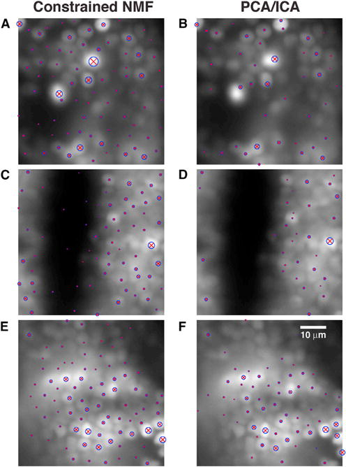
The patches are covered with the shape centers detected in that patch (blue circles around red “×” markers, with larger symbols indicating higher-ranked components), superimposed on the mean image for each patch.

(A, C, and E) Centers detected for the CNMF method, on patches containing the 1^st, 1,000^th, and 26,000^th ranked neurons, respectively.

(B, D, and F) Centers detected for the PCA/ICA method on the same patches. Calcium video and detected components in these patches can be viewed in Movies S2, S3, S4, S5, S6, and S7. The detected components for the PCA/ICA method are shown in Figure S2. Movie S8 shows the components detected throughout the brain, using CNMF.

In contrast, while the PCA/ICA method (Mukamel et al., 2009) usually performs well in locating “strong” neurons (i.e., high-SNR, well-separated neurons), this method misses many relatively “weak” neurons, as can be seen in Figures 6B, 6D, and 6F (see also Figure S2, and Movies S5, S6, and S7). PCA/ICA detects several thousand fewer high-quality components then the CNMF method with GL initialization in this dataset. Moreover, the components detected by CNMF usually have better quality than those detected by PCA/ICA. For example, the maximum DF/F traces of low-ranked components found by PCA/ICA are typically more noisy, attain smaller maximum values, and sometimes exhibit relatively strong negative values (Figure S2). In contrast, the CNMF method is able to denoise the activity and also obtain a non-negative signal (Figure 5). These results are consistent with those obtained in simulated data, as illustrated in Figures 2 and 3. Note that the method used here is closer to the plain NMF of Maruyama et al. (2014), with three key differences: (1) the NMF iterations here are spatially constrained to keep inferred components localized; (2) the GL initialization method allows us to process large patches of data at once and bypass the high level of manual intervention required by plain NMF; and (3) this new initialization method helps the CNMF iterations converge to a better solution.

Application to Dendritic Imaging Data

A key advantage of the proposed CNMF framework is that we can apply similar methods to imaging data focusing on the dendrites of multiple neurons and not on the cell bodies. In this case, each spatial component corresponds to a set of dendritic branches from a given neuron, and the temporal component corresponds to the synchronous activity of these branches. These data exhibit certain qualitative differences compared to somatic imaging. Each spatial component is again sparse but is no longer spatially localized, since dendritic branches can stretch significantly along the observed imaging plane. As a result, the degree of overlap between the different branches is significantly higher, making even rough interpretation by eye a challenging task; the correlation and mean images in this setting provide very little useful segmentation information (Figures 7A and 7C). Moreover, the bound calcium dynamics no longer follow somatic calcium indicator dynamics. Dropping the temporal dynamics and spatial localization constraints from our problem, we obtain a simpler sparse CNMF problem that can still be solved efficiently using the methods described above.

Figure 7. Application to In Vivo Dendritic Imaging Data from Rodent Barrel Cortex.

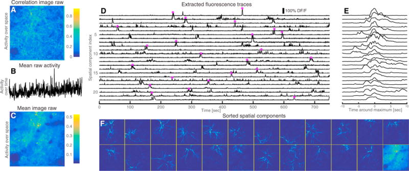
(A) Correlation image of the raw data. Due to the high degree of overlap, the correlation image cannot be used to segment the video.

(B) Spatially averaged activity over time of the raw data.

(C) Mean activity over time.

(D) DF/F temporal traces of the top 23 components extracted from our algorithm.

(E) Close up and centering around the point of maximum activation for each trace (indicated by the star marker in D).

(F) Sorted spatial footprints and background (lower right corner). The proposed method can segment the dense dendritic imaging data and reveal a rich underlying sparse structure (see also Movie S9).

We applied this approach to in vivo dendritic imaging data taken from the apical dendrites of layer 5 pyramidal neurons in the rodent barrel cortex (Lacefield and Bruno, 2013, SfN, abstract) and show the results in Figure 7. The raw data is typically dense when averaged over either time or space, as can be seen from the low intensity of the raw data correlation and mean image (Figures 7A–7C). We initialize randomly using a large number of components (in this case 50) and then order the inferred components as before. The top 23 of these components together with the background and the corresponding temporal traces in DF/F units are shown in Figures 7D–7F. These components are sparse in both space and time, with the temporal components extracting temporally localized bursts visible in the raw video data, and the spatial components extracting segments of the apparent dendritic structures visible in the video data (see also Movie S9). The results show the effectiveness of the sparse CNMF procedure in obtaining separated spatiotemporal components given dendritic imaging data in which the degree of overlap is very high and the spatial components are not localized.

DISCUSSION

A Flexible and Efficient Model for Calcium Deconvolution

The major contribution of this work is to introduce a framework for analysis of calcium imaging data that is (1) applicable to a large variety of data, (2) computationally efficient and parallelizable, and (3) user friendly, in the sense that the required human intervention is limited to the setting of a few intuitive parameters (e.g., rough estimates of number and size of neurons). This framework is enabled by a number of novel tools (CD, CNMF, efficient initialization, robust parameter estimation, and component sorting/merging) that can be combined in a modular fashion depending on the details of the imaging data (e.g., the spatiotemporal resolution). As a result, we were able to successfully apply our framework to many different imaging datasets without extensive specialized pre-processing.

Our CD approach builds upon and extends the fast nonnegative deconvolution (FOOPSI) method of Vogelstein et al., (2010) in several ways. Compared to FOOPSI, which permits only first-order autoregressive models with pre-specified time constant, our method allows for general AR (p) models and comes with a method for estimating the coefficients. More importantly, in the FOOPSI method, the loss function appears in the objective function, and a regularizer needs to be introduced and fine-tuned to control between the faithfulness to the observed data and the (unknown) sparsity of the underlying spiking signal. In our method, the tradeoff between sparsity and fidelity to observed data is set automatically by estimating the noise level a priori and using it as a hard constraint on the overall acceptable level of residual error, while retaining the same linear time computational complexity as FOOPSI.

Modeling the fluorescence trace with an AR process allows for a flexible and interpretable modeling framework that still retains computational tractability. When solving the CD problem, the complexity of the algorithm scales only with the order of the AR process and not with the length of the transient impulse response of the AR model, making this approach computationally more tractable than arbitrary template matching algorithms or blind deconvolution approaches (Diego-Andilla and Hamprecht, 2014). Moreover, the AR coefficients can be directly estimated from the raw data in a completely unsupervised way, do not require the existence of isolated spikes for fine-tuning the various parameters, and can be further fine-tuned during the deconvolution algorithm. Although this AR framework makes certain simplifying assumptions about the linearity and dynamics of the calcium indicator, nonetheless it results in a highly computationally efficient estimator that achieves state of the art performance among unsupervised methods, as shown recently in Theis et al. (2015).

CNMF Provides a Flexible Framework for Analysis of Large-Scale Calcium Imaging Data

We applied our framework to a diverse set of in vitro and in vivo imaging data to illustrate the wide applicability of the matrix factorization framework to large-scale imaging data. Matrix factorization inherently models the possible overlap between the different components as opposed to manual ROI selection or image segmentation-based techniques (Smith and Häusser, 2010; Kaifosh et al., 2014). Indeed, the matrix factorization approach often obtains highly overlapping spatial components in cases in which such components optimize the amount of variance explained in the data (up to the noise constraints). This contrasts with the PCA/ICA approach, which tends to reject overlapping areas in an attempt to seek maximally independent spatial components, at a risk of increased cross-talk and reduced SNR (Figures 2 and 3). As a result, our demixing method can be used in cases in which the spatial overlap is significant either naturally, because of the dense neural packing or deep imaging in scattering tissue, or artificially, due to the simultaneous observation of the projection of multiple z planes through spatial light modulation (Yang et al., 2015, companion paper), or more general projection patterns as suggested and studied in Pnevmatikakis and Paninski (2013); such approaches may lead to computational imaging schemes that allow us to simultaneously image larger neural populations than would be otherwise possible and are an important direction for future research.

The iterative factorization procedure is largely agnostic regarding the shape of the spatial components, inferring these shapes directly from the data with few prior constraints. Other approaches, especially for analysis of somatic imaging data (Pachitariu et al., 2013; Diego-Andilla and Hamprecht, 2014), use dictionary learning approaches to learn a compact basis for the representation of the spatial footprints. These methods can help reduce the dimensionality of the problem and can be helpful in more macroscopic images in which detailed structure is not available. In future work, it may be useful to combine these methods with the techniques developed here. However, these dictionary-learning methods do not appear to generalize to more microscopic imaging (e.g., dendritic imaging; Figure 7), where the structure of the spatial components can be rich and unpredictable.

Sparse and structured NMFs have been proposed in the recent literature (Pnevmatikakis and Paninski, 2013; Diego-Andilla and Hamprecht, 2013; Haeffele et al., 2014) in an attempt to constrain the factorization procedure and produce compact spatial footprints and denoised temporal traces. The structure there is promoted by the inclusion of regularizers that promote certain desired characteristics. For example, Pnevmatikakis and Paninski (2013) propose a nuclear norm penalty to identify the number and initialize the spatial components. Haeffele et al. (2014) propose the inclusion of a spatial total variation norm penalty to promote localized and compact spatial footprints. Diego-Andilla and Hamprecht (2014) propose a sparse space-time deconvolution for learning the neuron locations and extracting spike activity through dictionary learning and blind deconvolution. A typical drawback of these approaches is the need to tune regularization weights. Moreover, a single regularizer over the observed field of view implicitly assumes that the statistics are uniform across the whole observed field of view: i.e., the density and size of neurons is uniform, all the neurons fire at similar average rates, and the noise power across the observed field of view is similar. These assumptions can often lead to the omission of weaker components and require the processing of small patches at a time as noted by Maruyama et al. (2014). A distinctive feature of the CNMF framework presented here is that this regularization approach is replaced by a larger set of constraints on the noise power at each pixel. These noise levels are automatically estimated a priori and implicitly impose non-uniform statistics on the observed field of view.

A Modular Approach toward Automated Calcium Imaging Data Analysis

Our approach is highly modular and provides a flexible analysis framework. For example, depending on the imaging frame rate, the deconvolution step can be turned on or off, or the proposed CD framework can be replaced by other methods (e.g., particle filtering [Vogelstein et al., 2010], greedy optimization [Grewe et al., 2010], or MCMC [Pnevmatikakis et al., 2013]). Different neurons can have the same or different time constants that can also be re-estimated using the proposed AR approach. Our initialization algorithms target cell bodies whose images can be crudely modeled as Gaussians with specific sizes, although different shapes can be easily incorporated.

A specific objective in this work was to create a framework that requires minimal human intervention. In our models, the parameters that are user defined are specified during the initialization procedures and pertain to the number of components that are sought initially (greedy initialization, and sparse NMF in the case of dendritic imaging), and/or the size/scale of the spatial components that are sought (greedy, GL initialization). The rest of the parameters (noise levels, calcium indicator dynamics, time-varying baseline concentration) are tuned automatically, though again, any prior knowledge about these quantities can be readily incorporated. While this level of human intervention is low, it remains an important open problem to automatically estimate the number or the size of the imaged components. To that end, we also introduced a measure that ranks the inferred components in terms of their significance, and correction moves that merge overlapping and correlated components, or remove insignificant components, and found that such moves can be very helpful in practice (Figures 4, 5, 6, and 7).

Calcium imaging as a neural recording method can provide rich and diverse datasets depending on many factors (imaging technique, experimental conditions, calcium indicators, etc.), and multineuronal data with spiking and/or spatial anatomical ground truth remains scarce and typically hard to obtain. Moreover, assessing the performance of different approaches remains an open issue, with no universally accepted performance measure. For example, the spike correlation metric used in this study to quantify the performance of activity deconvolution methods is empirically very sensitive to spike jitter. The situation is even more complicated in automatically quantifying the performance of spatial footprint identification methods. Simple correlation-based metrics, for example, can be insensitive to the detailed morphological structure, and even the comparison against ground truth data (e.g., through dual channel labeling) can be challenging due to potential spatial overlap, poor expression, or unmodeled background activity. As such, the goal of a globally operating algorithm that requires no human intervention and has performance guarantees remains elusive. Nevertheless, we hope that the family of methods discussed here, under the unifying umbrella of CNMF, will provide a useful framework for future research.

EXPERIMENTAL PROCEDURES

Experimental Data

Full details on the experimental data are provided in the Supplemental Experimental Procedures.

Data Analysis

All analysis was performed with custom-written MATLAB (RRID: nlx_153890) code. MATLAB and Python implementations of the CD and CNMF algorithms can be found in https://github.com/epnev/ca_source_extraction and linked repositories therein.

Autoregressive Model for Calcium Dynamics

We assume we observe the fluorescence signal for T timesteps and denote by s(t) the number of spikes that the neuron fired at the t-th timestep, t = 1,…, T. We approximate the calcium concentration dynamics c using a stable autoregressive process of order p(AR(p)) where p is a small positive integer,

$$c(t)={\displaystyle {\sum }_{j=1}^p{\mathrm{\gamma }}_{j}c(t-j)+s}(\mathrm{t}).$$ (Equation 1)

If p = 1 then the calcium transient in response to a spike is modeled by an instantaneous-increase slowly decaying exponential function. This is recommended when the rise time constant is small compared to the length of the timebin. In case we want to explicitly model the rise time, we choose p = 2. More structured responses (e.g., multiple decay time constants) can also be modeled with higher values for the order p. The observed fluorescence is related to the calcium concentration as:

$$y(t)=\alpha (c(t)+b)+\epsilon (t),\epsilon (t)~\mathcal{N}(0,{\sigma }^2),$$ (Equation 2)

where α is a nonnegative scalar, b is the baseline concentration and the noise is assumed to be i.i.d. zero mean Gaussian with variance σ². The goal of calcium deconvolution is to extract an estimate of the neural activity s from the vector of observations y.

Estimation of Model Parameters

For a given order p and under the assumption that the spiking signal s comes from a homogeneous Poisson process, the autocovariance function of y, C_y satisfies the recursion:

$$C_y(\tau )=\{\begin{array}{cc}{\displaystyle {\sum }_{j=1}^p{\mathrm{\gamma }}_j{C}_y(\tau -j)-{\sigma }^2{\mathrm{\gamma }}_{\tau },}& 1\le \tau \le p\\ {\displaystyle {\sum }_{j=1}^p{\mathrm{\gamma }}_j{C}_y(\tau -j),}& \tau >p.\end{array}$$ (Equation 3)

By plugging the sample autocovariance values into Equation 3, we can first estimate the AR coefficients γ₁, …, γ_p. While Equation 3 can also be used to estimate the noise variance σ², a more robust estimate can be obtained by observing the power spectral density (PSD) of y. The uncorrelated additive noise has flat PSD, whereas the PSD due to the calcium signal decays with the frequency as ~(1/f²). At high frequencies, and under sparse spiking, the PSD will be dominated by the noise, and therefore an estimate ${\widehat{\sigma }}^2$ can be obtained by averaging the PSD over a range of high frequencies. We discuss these issues in more detail in the Supplemental Information (Figure S1).

Sparse, Nonnegative, Noise-Constrained Deconvolution

Solving for the spiking vector s in the domain of nonnegative integers is a computationally hard problem and also requires knowledge of the spike amplitude scaling constant α, which is in general unavailable. Instead, by following the approach in Vogelstein et al. (2010), we can absorb α into s, relax s to take arbitrary nonnegative values, and penalize the sum of the spike signal over time (which can be seen as the l₁-norm of a nonnegative signal), to promote spike sparsity and avoid overfitting. First note that Equation 1 can be expressed in matrix form as Gc = s, with

$$G=\left[\begin{array}{ccccc}\hfill 1\hfill & \hfill 0\hfill & \hfill 0\hfill & \hfill \dots \hfill & \hfill 0\hfill \\ \hfill -{\mathrm{\gamma }}_1\hfill & \hfill 1\hfill & \hfill 0\hfill & \hfill \dots \hfill & \hfill 0\hfill \\ \hfill -{\mathrm{\gamma }}_2\hfill & \hfill -{\mathrm{\gamma }}_1\hfill & \hfill 1\hfill & \hfill \dots \hfill & \hfill 0\hfill \\ \hfill ⋮\hfill & \hfill \ddots \hfill & \hfill \ddots \hfill & \hfill \ddots \hfill & \hfill ⋮\hfill \\ \hfill 0\hfill & \hfill \dots \hfill & \hfill -{\mathrm{\gamma }}_2\hfill & \hfill -{\mathrm{\gamma }}_1\hfill & \hfill 1\hfill \end{array}\right].$$ (Equation 4)

(Note that we have ignored initial conditions for notational simplicity.)

Now based on the estimate of the noise variance, we can introduce a hard constraint on the residual energy; from Equation 2, we have that for each time $\mathbb{E}{\left(y\left(t\right)-\alpha \left(c\left(t\right)+b\right)\right)}^2={\sigma }^2$. Summing over all timesteps, we find that the residual vector satisfies $\mathbb{E}{\Vert \mathit{y}-\alpha (\mathit{c}+b{\mathbf{1}}_T)\Vert }^2={\sigma }^{2}T$ (with 1_T a column vector of ones with length T); moreover, by the law of large numbers ${\Vert \mathit{y}-\alpha (\mathit{c}+b{\mathbf{1}}_T)\Vert }^2\approx {\sigma }^{2}T$ with high probability. We can use this estimate to derive the following convex program for estimating the calcium concentration up to a scaling constant:

$$\begin{array}{ll}\underset{\widehat{\mathit{c}},\widehat{b},\widehat{\mathit{s}}}{min}& 1_T^{\mathrm{T}}\widehat{\mathit{s}}\\ \text{subject to}:& \widehat{\mathit{s}}\ge 0,\widehat{\mathit{s}}=G\widehat{\mathit{c}},\Vert \mathit{y}-\widehat{\mathit{c}}-\widehat{b}{\mathbf{1}}_T\Vert \le \widehat{\sigma }\sqrt{T}.\end{array}$$ (P-CD)

Program (P-CD) also estimates the baseline concentration b, which for now is assumed to be constant; we relax this assumption in the spatiotemporal case. However, in many cases the baseline can be estimated a priori, e.g., by averaging the fluorescence over a large interval with no observed spikes.

Program (P-CD) is convex and a global optimum exists and is achievable with standard optimization methods that computationally scale only linearly with the number of observed timesteps; this enables the analysis of long time series or videos. A variety of methods can be used to solve (P-CD) in linear time, as detailed in the Supplemental Experimental Procedures.

Note that the CD approach can estimate the $\widehat{\mathit{s}}$ (or $\widehat{\mathit{c}}$), only up to a multiplicative constant, since the amplitude of a single spike bin terms of fluorescence response (α in Equation 2) is in general unknown and in general cannot be readily estimated. If needed, estimates of the spike amplitude can be derived using the MCMC algorithm of Pnevmatikakis et al. (2013).

Updating the Time Constants

The time constants are updated in the continuous time domain, by using a simple MCMC scheme. Details are given in the Supplemental Experimental Procedures.

Spatiotemporal Deconvolution and Component Demixing

Now we turn to the full spatiotemporal case. At every timestep, a field of view is observed for a total number of T timesteps. This field (either two- or three-dimensional) has a total number of d pixels/voxels and the observations at any point in time can be vectorized in a single column vector of length d. Thus, all the observations can be described by a d × T matrix Y. Now assume that the field contains a total number of (possibly overlapping) K neurons, where K is assumed known for now. For each neuron i the neural activity s_i and “calcium activity” c_i can be described again with the AR(p) dynamics of Equation 1. Now if ${\mathbf{a}}_i\in {\mathbb{R}}_{+}^d$ denotes the (nonnegative) “spatial footprint” for neuron i (written in vector form), then we model the spatial calcium concentration profile at time t as

$$F(t)={\displaystyle \sum _{i=1}^K{\mathbf{a}}_i{c}_i(t)+B(t)},$$ (Equation 5)

where $B(t)\in {\mathbb{R}}_{+}^d$ denotes the (time-varying) baseline vector all the pixels. Finally, at each timestep we observe F(t) corrupted by additive Gaussian noise:

$$Y(t)=F(t)+\epsilon (t),\epsilon (t)~\mathcal{N}(\mathbf{0},\sum )$$ (Equation 6)

where Σ is a diagonal matrix (indicating that the noise is spatially and temporally uncorrelated). These equations can be written in matrix form as

$$\begin{array}{l}S=C{G}^T\\ F=AC+B\\ Y=F+E,\end{array}$$

with S = [s₁,…, s_K]^T, C= [c₁,…, c_K]^T, A = [a₁,…, a_K], F = [F(1), F(2),…, F(T)], E = [ε(1) ε(2),…, ε(T)], Y = [Y(1), Y(2),…, Y(T)], B= [B(1), B(2),…, B(T)], and G is defined in Equation 4. In practice, we have found that the background activity matrix B can often be modeled as a rank 1 matrix, B = bf^T, where $\mathbf{b}\in {\mathbb{R}}_{+}^d$, $\mathbf{f}\in {\mathbb{R}}_{+}^{\mathrm{T}}$ are nonnegative vectors encoding the background spatial structure (typically consisting of a sum of baseline activity from the neurons of interest and densely mixed neuropil structure below the observed spatial field) and global (time varying) intensity, respectively.

CNMF Framework

We approach this problem by employing a CNMF framework to infer the key parameters of interest (the spatial components A and temporal components C) along with b,f, and Σ. The factorization procedure itself is constrained in a number of ways. (1) The residual between the observed data and the reconstructed video is bound by similar noise power constraints as in the time series deconvolution case, where now we estimate a different noise level for each observed pixel/voxel, again from the temporal PSD. (2) Both the spatial and the temporal components are endowed with non-negativity constraints. (3) The spatial components are also constrained to be sparse, promoting more compact, regularized spatial footprints. Finally, (4) when the observed imaging rate is much higher than the decay rate of the indicator, we constrain the temporal traces to obey the indicator dynamics, similarly to the one-dimensional case. With this set of constraints, we can optimize the spatial and temporal components in an iterative alternating way, where a new estimate for A and b is obtained given the last estimate of C and f and vice versa, within the space defined by the constraints. At the end of each iteration, additional steps are introduced, where overlapping components that exhibit significant temporal correlations are merged into a single component, and existing components that do not contribute significant activity are removed and absorbed into the background. We also present two different methods for initializing the spatial components.

Our framework can be summarized into the following steps:

1. Determine the AR dynamics and noise power for each voxel.

2. Initialize A, b, C, f through one of the initialization procedures.

3. Update components A, b, C, f using constrained alternating matrix factorization.

4. Merge and/or remove existing components.

5. Repeat steps 3 and 4.

Iterative Matrix Updates

Assuming the number of neurons K and initial estimates of A, C and b, f as known, we can apply alternating matrix factorization methods to estimate the spatial components A, b given the temporal C, f and vice versa, from the fluorescence observations Y.

Estimating A, b

Since each column of A expresses the location and shape of a neuron, we want A to be sparse to promote localized spatial footprints. Again, this is done by minimizing the l₁ norm of A, which equals the sum of all its entries, since A is constrained to be non-negative. Given estimates of C^(k−1) and f^(k−1) from the previous iteration, the spatial matrix A^(k) and background b^(k) can be updated by solving the following convex program

$$\begin{array}{l}{\min }_{A,\mathbf{b}}{\Vert A\Vert }_1,\hfill \\ \text{subject to}:\mathrm{A},\mathbf{b}\ge 0,\Vert Y(i,:)-A(i,:)C^{(k-1)}-b(i){\mathit{f}}^{(k-1)T}\Vert \le {\sigma }_i\sqrt{T},i=1,\dots d,\hfill \end{array}$$ (P-S)

where A(i,:); Y(i,:) denote the i-th rows of A and Y, respectively. Although the matrix A is of very large size, d × T, the problem (P-S) can be readily parallelized into d programs for each pixel separately. Similarly to the CD problem (P-CD), each of these problems can be solved with a variety of methods (see the Supplemental Experimental Procedures).

When the fluorescence from each neuron is highly localized near the soma, the process of estimating A at the k-th iteration can be further sped up and regularized by restricting the candidate spatial support of cell j at the iteration k, to be a mildly dilated version of the support as is determined by the column j of A^(k−1). When estimating the i-th row of A^(k), we can restrict our search to the neurons (columns of A) whose candidate support sets include the pixel i. This makes the dimensionality of each subproblem much smaller, leading to a highly efficient and parallelizable update.

Note that we have not yet incorporated any prior information about the detailed shape of the spatial components A(:, i), which enabled the highly parallel approach described above. However, in many cases it is natural to assume that A(:, i) is connected, or smooth in a suitable sense. Empirically, we have found it helpful to include a mild post-processing step at each iteration, using standard non-linear image filtering techniques, such as median filtering or morphological opening, which are effective in removing isolated pixels that appear as active. The removed pixels can then be absorbed by the background component.

Estimating C, f

For the temporal components, we want to introduce a sparsity penalty to the activity of each neuron to prevent overfitting. We can again use our estimates of the noise variance as hard constraints and derive a parameter-free convex program:

$$\begin{array}{c}{min}_{{\mathit{c}}_1,{\mathit{c}}_2,\dots ,{\mathit{c}}_k,\mathit{f}}{\displaystyle {\sum }_{j=1}^K{\mathbf{1}}^T\mathrm{G}{\mathit{c}}_j}\\ \text{subject to}:\mathrm{G}{\mathit{c}}_j\ge \mathbf{0},j=1,\dots ,K,\Vert Y\left(i,:\right)-A\left(i,:\right)C^{\left(k-1\right)}-b\left(i\right){\mathbf{f}}^{\left(k-1\right)T}\Vert \le {\sigma }_i\sqrt{T},i=1,\dots ,d\end{array}$$ (P-T)

Since the constraints Gc_i ≥ 0 couple the entries within each row of C, and the residual constraints act within each column, the program (P-T) cannot be readily parallelized. Moreover, the large number of constraints and the potentially large number of neurons K make the direct solution of (P-T) computationally expensive. To overcome this, we employ a partially parallelizable block-coordinate descent approach, where we sequentially update the temporal component c_j of one neuron at a time; nonoverlapping components can be updated in parallel.

Incorporating Different Deconvolution Methods

The method for updating the temporal components C, f is a simple spatiotemporal extension of the CD method presented earlier. However, in principle, any time series deconvolution method can be used as part of our CNMF framework. To do so, we can construct for each component, a trace that represents the raw data, averaged over the corresponding spatial footprint, after the activity of all the other components has been removed. More specifically, if we want to compute the j-th temporal component at the k-th iteration ${\mathbf{c}}_j^{(k)}$, provided we have computed ${\mathbf{c}}_j^{(k)},\dots ,{\mathbf{c}}_{j-1}^{(k)}$, ${\mathbf{c}}_{j+1}^{(k-1)},\dots ,{\mathbf{c}}_K^{(k-1)}$ we can form the quantity

$${\left({\mathbf{y}}_j^{(k)}\right)}^{\mathrm{T}}=\frac{{\left({\mathbf{a}}_j^{(k)}\right)}^{\mathrm{T}}}{{\Vert {\mathbf{a}}_j^{(k)}\Vert }^2}\left(Y-\left[{\mathbf{a}}_1^{(k)},\dots ,{\mathbf{a}}_{j-1}^{(k)},{\mathbf{a}}_{j+1}^{(k)},\dots ,{\mathbf{a}}_K^{(k)}\right]{\left[{\mathbf{c}}_1^{(k)},\dots ,{\mathbf{c}}_{j-1}^{(k)},{\mathbf{c}}_{j+1}^{(k-1)},\dots ,{\mathbf{c}}_K^{(k-1)}\right]}^{\mathrm{T}}-{\mathbf{b}}^{(k)}{\left({\mathbf{f}}^{(k-1)}\right)}^{\mathrm{T}}\right),$$ (Equation 7)

and then apply our deconvolution method of choice to ${\mathbf{y}}_j^{(k)}$ to obtain ${\mathbf{c}}_j^{(k)}$. This scheme adds flexibility and enables the different treatment of different components, in terms of time constants/dynamics, noise levels, etc.

Merging Existing Components

At the end of each iteration, we seek spatially overlapping components with temporal correlations above a certain threshold. These components are then merged into a single component. Details are given in the Supplemental Experimental Procedures.

Ranking and Removing Components

Identifying the number of components a priori is a challenging problem. While the GL initialization approach (see below) offers an adaptive method to estimate this number, and the merge operations aim to correct for false estimates, it is usually difficult to automatically identify all the correct components without any false positives. As a strategy we have found that it is more effective to overestimate the number of components and then remove those that do not correspond to neural activity. To do this, we sort the components according to the product of the maximum values of the temporal and spatial components. Empirically, we find that the first components in the list have compact footprints and strong temporal activity, making it easy for the user to set a cutoff $\widehat{K}$ above which the obtained activity is retained, and below which the components are discarded. The discarded components can then be absorbed into the background.

Greedy Initialization for Somatic Imaging Data

At every iteration, the residual of the spatiotemporal data matrix (or, in the first iteration, the data matrix itself) is spatially filtered with a Gaussian kernel of width similar to the size of a cell body. The algorithm finds the location where this filtering procedure explains the maximum variance and selects a square of size roughly twice the size of an average neuron. Within this square, a rank-1 NMF is performed to initialize the spatial and temporal components, and the product of these components is then subtracted from the observed data to form the new spatiotemporal residual. This procedure is repeated until a user-specified number of components is located; note that the different components obtained across all iterations are allowed to overlap. Then, the resulting residual signal is used to initialize the background component B = bf^T, again using rank-1 NMF (see Supplemental Experimental Procedures for implementation details).

Group Lasso Initialization for Somatic Imaging Data

The greedy initialization method can be problematic if neurons are packed too densely, especially if their activities are highly correlated. In this case, we use a different approach, where we initially assume that a potential neuron with a Gaussian shape of fixed size is centered at every observed voxel, and denote by X the d × T activity matrix of all these potential neurons. We then seek to minimize the number of active neurons that can explain the observed spatiotemporal data. We adopt a GL (Yuan and Lin 2006) approach, and form the following convex optimization problem

$${min}_{X\in {\mathbb{R}}_{+}^{d\times T},\mathbf{b}\in {\mathbb{R}}^d}{\Vert Y-DX-\mathbf{b}{\mathbf{1}}_T^{\mathrm{T}}\Vert }_F^2+\lambda {\displaystyle \sum _i\sqrt{{\displaystyle \sum _t{X}_{\mathit{it}}^2,}}}$$ (Equation 8)

where again the data is given by Y∈ℝ^d × ^T, λ, λ is a regularization constant, and D∈ℝ^d × ^d is a matrix which performs convolution with a Gaussian kernel in the original spatial coordinates. We infer the underlying neuronal activity X and the background component $\mathbf{b}{\mathbf{1}}_T^{\mathrm{T}}$. We use each column of D (which corresponds to a Gaussian kernel at each location) as a hypothetical neuron and select the significant locations by solving a GL problem Equation 8, where each group corresponds to the temporal activity of a hypothetical neuron. The GL penalty $\lambda {\displaystyle {\sum }_i\sqrt{{\displaystyle {\sum }_t{X}_{\mathit{it}}^2}}}$ forces locations with sufficiently low activity to have precisely zero activity ( ${\displaystyle {\sum }_t{X}_{\mathit{it}}^2=0}$ for these locations i). The resulting “significant” locations i, in which X_it > 0, give an estimate of a neuron’s spatial footprint. However, the neuron centers cannot be identified simply by using all the nonzero locations, since one real neuron usually makes all the nearby locations have significant activity. Therefore, we identify regional maxima of ${\displaystyle {\sum }_t{X}_{\mathit{it}}^2}$ as the neuron centers. Note that by moderately sacrificing convexity, the procedure can be extended to include a time-varying baseline component f. The initialization to the matrix factorization approach is then given by the detected $\widehat{K}$ components, each with a Gaussian shape a_k centered around the identified neuron centers and activity c_k given by the averaging X(i,:) over all non-zero locations i, which are closest to the center. Implementation details are given in the Supplemental Experimental Procedures.

Highlights.

• We present a new method for analyzing large-scale calcium imaging datasets

• The method identifies the cell locations and deconvolves their neural activity

• Applications to in vivo somatic and dendritic imaging are presented

• We make available MATLAB and Python implementations of our method

References

- Ahrens MB, Orger MB, Robson DN, Li JM, Keller PJ. Whole-brain functional imaging at cellular resolution using light-sheet microscopy. Nat Methods. 2013;10:413–420. doi: 10.1038/nmeth.2434. [DOI] [PubMed] [Google Scholar]
- Chen TW, Wardill TJ, Sun Y, Pulver SR, Renninger SL, Baohan A, Schreiter ER, Kerr RA, Orger MB, Jayaraman V, et al. Ultrasensitive fluorescent proteins for imaging neuronal activity. Nature. 2013;499:295–300. doi: 10.1038/nature12354. [DOI] [PMC free article] [PubMed] [Google Scholar]
- Cotton RJ, Froudarakis E, Storer P, Saggau P, Tolias AS. Three-dimensional mapping of microcircuit correlation structure. Front Neural Circuits. 2013;7:151. doi: 10.3389/fncir.2013.00151. [DOI] [PMC free article] [PubMed] [Google Scholar]
- Diego-Andilla F, Hamprecht FA. Learning multi-level sparse representations. In: Burges CJC, Bottou L, Welling M, Ghahramani Z, Weinberger KQ, editors. Advances in Neural Information Processing Systems 26 (NIPS 2013) Curran Associates; 2013. pp. 818–826. [Google Scholar]
- Diego-Andilla F, Hamprecht FA. Sparse space-time deconvolution for calcium image analysis. In: Ghahramani Z, Welling M, Cortes C, Lawrence ND, Weinberger KQ, editors. Advances in Neural Information Processing Systems 27 (NIPS 2014) Curran Associates; 2014. pp. 64–72. [Google Scholar]
- Duemani Reddy G, Kelleher K, Fink R, Saggau P. Three-dimensional random access multiphoton microscopy for functional imaging of neuronal activity. Nat Neurosci. 2008;11:713–720. doi: 10.1038/nn.2116. [DOI] [PMC free article] [PubMed] [Google Scholar]
- Freeman J, Vladimirov N, Kawashima T, Mu Y, Sofroniew NJ, Bennett DV, Rosen J, Yang CT, Looger LL, Ahrens MB. Mapping brain activity at scale with cluster computing. Nat Methods. 2014;11:941–950. doi: 10.1038/nmeth.3041. [DOI] [PubMed] [Google Scholar]
- Grewe BF, Langer D, Kasper H, Kampa BM, Helmchen F. High-speed in vivo calcium imaging reveals neuronal network activity with near-millisecond precision. Nat Methods. 2010;7:399–405. doi: 10.1038/nmeth.1453. [DOI] [PubMed] [Google Scholar]
- Haeffele B, Young E, Vidal R. Structured low-rank matrix factorization: optimality, algorithm, and applications to image processing. Xing EP, Jebara T, editors. Proceedings of the 31st International Conference on Machine Learning. 2014:2007–2015. http://jmlr.org/proceedings/papers/v32/haeffele14.pdf.
- Kaifosh P, Zaremba JD, Danielson NB, Losonczy A. SIMA: Python software for analysis of dynamic fluorescence imaging data. Front Neuroinform. 2014;8:80. doi: 10.3389/fninf.2014.00080. [DOI] [PMC free article] [PubMed] [Google Scholar]
- Machado TA, Pnevmatikakis E, Paninski L, Jessell TM, Miri A. Primacy of Flexor Locomotor Pattern Revealed by Ancestral Reversion of Motor Neuron Identity. Cell. 2015;162:338–350. doi: 10.1016/j.cell.2015.06.036. [DOI] [PMC free article] [PubMed] [Google Scholar]
- Maruyama R, Maeda K, Moroda H, Kato I, Inoue M, Miyakawa H, Aonishi T. Detecting cells using non-negative matrix factorization on calcium imaging data. Neural Netw. 2014;55:11–19. doi: 10.1016/j.neunet.2014.03.007. [DOI] [PubMed] [Google Scholar]
- Mukamel EA, Nimmerjahn A, Schnitzer MJ. Automated analysis of cellular signals from large-scale calcium imaging data. Neuron. 2009;63:747–760. doi: 10.1016/j.neuron.2009.08.009. [DOI] [PMC free article] [PubMed] [Google Scholar]
- Nikolenko V, Watson BO, Araya R, Woodruff A, Peterka DS, Yuste R. SLM Microscopy: Scanless Two-Photon Imaging and Photostimulation with Spatial Light Modulators. Front Neural Circuits. 2008;2:5. doi: 10.3389/neuro.04.005.2008. [DOI] [PMC free article] [PubMed] [Google Scholar]
- Oñativia J, Schultz SR, Dragotti PL. A finite rate of innovation algorithm for fast and accurate spike detection from two-photon calcium imaging. J Neural Eng. 2013;10:046017. doi: 10.1088/1741-2560/10/4/046017. [DOI] [PMC free article] [PubMed] [Google Scholar]
- Pachitariu M, Packer AM, Pettit N, Dalgleish H, Hausser M, Sahani M. Extracting regions of interest from biological images with convolutional sparse block coding. In: Burges CJC, Bottou L, Welling M, Ghahramani Z, Weinberger KQ, editors. Advances in Neural Information Processing Systems 26 (NIPS 2013) Curran Associates; 2013. pp. 1745–1753. [Google Scholar]
- Pnevmatikakis EA, Paninski L. Burges CJC, Bottou L, Welling M, Ghahramani Z, Weinberger KQ. Advances in Neural Information Processing Systems 26 (NIPS 2013) Curran Associates; 2013. Sparse nonnegative deconvolution for compressive calcium imaging: algorithms and phase transitions; pp. 1250–1258. [Google Scholar]
- Pnevmatikakis EA, Merel J, Pakman A, Paninski L. Bayesian spike inference from calcium imaging data. 2013 Asilomar Conference on Signals, Systems and Computers. 2013:349–353. http://dx.doi.org/10.1109/ACSSC.2013.6810293.
- Prevedel R, Yoon YG, Hoffmann M, Pak N, Wetzstein G, Kato S, Schrödel T, Raskar R, Zimmer M, Boyden ES, Vaziri A. Simultaneous whole-animal 3D imaging of neuronal activity using light-field microscopy. Nat Methods. 2014;11:727–730. doi: 10.1038/nmeth.2964. [DOI] [PMC free article] [PubMed] [Google Scholar]
- Rochefort NL, Garaschuk O, Milos RI, Narushima M, Marandi N, Pichler B, Kovalchuk Y, Konnerth A. Sparsification of neuronal activity in the visual cortex at eye-opening. Proc Natl Acad Sci USA. 2009;106:15049–15054. doi: 10.1073/pnas.0907660106. [DOI] [PMC free article] [PubMed] [Google Scholar]
- Smith SL, Häusser M. Parallel processing of visual space by neighboring neurons in mouse visual cortex. Nat Neurosci. 2010;13:1144–1149. doi: 10.1038/nn.2620. [DOI] [PMC free article] [PubMed] [Google Scholar]
- Theis L, Berens P, Froudarakis E, Reimer J, Rosón MR, Baden T, Euler T, Tolias A, Bethge M. Supervised learning sets benchmark for robust spike detection from calcium imaging signals. 2015;arXiv arXiv:1503.00135, http://arxiv.org/abs/1503.00135. [Google Scholar]
- Vogelstein JT, Watson BO, Packer AM, Yuste R, Jedynak B, Paninski L. Spike inference from calcium imaging using sequential Monte Carlo methods. Biophys J. 2009;97:636–655. doi: 10.1016/j.bpj.2008.08.005. [DOI] [PMC free article] [PubMed] [Google Scholar]
- Vogelstein JT, Packer AM, Machado TA, Sippy T, Babadi B, Yuste R, Paninski L. Fast nonnegative deconvolution for spike train inference from population calcium imaging. J Neurophysiol. 2010;104:3691–3704. doi: 10.1152/jn.01073.2009. [DOI] [PMC free article] [PubMed] [Google Scholar]
- Yang W, Miller JK, Carrillo-Reid L, Pnevmatikakis EA, Paninski L, Yuste R, Peterka DS. Simultaneous multiplane imaging of neural circuits. Neuron. 2015;89:269–284. doi: 10.1016/j.neuron.2015.12.012. this issue. [DOI] [PMC free article] [PubMed] [Google Scholar]
- Yuan M, Lin Y. Model selection and estimation in regression with grouped variables. J R Stat Soc Series B Stat Methodol. 2006;68:49–67. [Google Scholar]
Associated Data
This section collects any data citations, data availability statements, or supplementary materials included in this article.