Dynamic PET simulator via tomographic emission projection for kinetic modeling and parametric image studies

Abstract

Purpose:

To develop and evaluate a fast and simple tool called dpetstep (Dynamic PET Simulator of Tracers via Emission Projection), for dynamic PET simulations as an alternative to Monte Carlo (MC), useful for educational purposes and evaluation of the effects of the clinical environment, postprocessing choices, etc., on dynamic and parametric images.

Methods:

The tool was developed in matlab using both new and previously reported modules of petstep (PET Simulator of Tracers via Emission Projection). Time activity curves are generated for each voxel of the input parametric image, whereby effects of imaging system blurring, counting noise, scatters, randoms, and attenuation are simulated for each frame. Each frame is then reconstructed into images according to the user specified method, settings, and corrections. Reconstructed images were compared to MC data, and simple Gaussian noised time activity curves (GAUSS).

Results:

dpetstep was 8000 times faster than MC. Dynamic images from dpetstep had a root mean square error that was within 4% on average of that of MC images, whereas the GAUSS images were within 11%. The average bias in dpetstep and MC images was the same, while GAUSS differed by 3% points. Noise profiles in dpetstep images conformed well to MC images, confirmed visually by scatter plot histograms, and statistically by tumor region of interest histogram comparisons that showed no significant differences (p < 0.01). Compared to GAUSS, dpetstep images and noise properties agreed better with MC.

Conclusions:

The authors have developed a fast and easy one-stop solution for simulations of dynamic PET and parametric images, and demonstrated that it generates both images and subsequent parametric images with very similar noise properties to those of MC images, in a fraction of the time. They believe dpetstep to be very useful for generating fast, simple, and realistic results, however since it uses simple scatter and random models it may not be suitable for studies investigating these phenomena. dpetstep can be downloaded free of cost from https://github.com/CRossSchmidtlein/dPETSTEP.

1. INTRODUCTION

Dynamic positron emission tomography (PET) plays an important role in in-vivo quantification of physiological processes in organs and tissues. In the field of oncology, the estimation of model based physiological parameters can provide a more accurate diagnosis, and aid in the screening, prediction, staging, treatment planning, and segmentation of cancerous tumors, as well as enable better treatment follow-up.^1–5 Parameters estimated for tumor regions of interest (ROIs), as well as full parametric images have proved to be efficient aids in tumor delineation^6–8 and treatment monitoring.^6,9,10 However, in order to obtain reliable and actionable kinetic parameters one has to have knowledge about sources and magnitude of bias and uncertainty associated with these derived parameters, and how they are affected by the acquisition environment and reconstruction parameter choices. In this study we introduce a fast dynamic PET simulator, based on the petstep (PET Simulator of Tracers via Emission Projection) platform,¹¹ that will allow researchers to better understand the bias and uncertainty tradeoffs as a function of the clinical environment and various postprocessing choices, such as reconstruction parameters, postfiltering, and parameter fitting models.

There are a number of methods to provide insight in the different aspects of dynamic PET and kinetic modeling, and the three main approaches are:

• 1.Image approach. Data from real patients or phantom PET scans is used.
• 2.Plain sinogram or time activity curve (TAC) simulation. Ideal sinograms or TACs are simulated and different amounts of variability and noise are added to mimic real PET data. The added noise comes from a known distribution, typically Poisson in projection space or Gaussian in image space.
• 3.Monte Carlo (MC) simulations. Simulates a digital patient or phantom undergoing a complete PET scan and reconstruction process, with sources of noise and variability coming from accurate modeling of the physical decay, photon transport in matter, and image reconstruction method of noisy data.

Some of the image approaches use phantoms. However, at present even state-of-the-art phantoms are limited since they do not support full dynamics with known kinetic parameters. As a result, they cannot be used to estimate, e.g., the optimal time weights to use for model fitting.

The second alternative, plain sinogram or TAC simulations, solves part of this problem, since the “true” or reference values are known. However, a major issue with this approach is that the TACs are generally simulated independently from one another. This is not realistic due to correlations introduced during the reconstruction process. This is especially true for nonlinear iterative reconstruction algorithms such as ordered-subset expectation maximization (OSEM),¹² in which the convergence of the method is heavily object-dependent, making noise properties vary across the image.^13–16 As a result, the plain sinogram/TAC approach is better suited for ROI analysis where individual voxel kinetics is of less interest. Another issue with the plain simulation approach is that noise properties in reconstructed images, and hence image-derived TACs, are typically not easily described as a simple Gaussian or Poisson distribution, but are instead more complex and not easily computed.^13,17,18 Therefore, adding noise using simple distributions does not as accurately represent the bias and variance compared to image-derived TACs. Nonetheless, simulations of these kinds are readily used in nuclear medicine.

The golden standard simulation method today is MC. The effects of, e.g., positron range, camera system blurring, image reconstruction process and so on can be included. This fact makes MC simulations a suitable choice for studies of tumor heterogeneity, time sampling scheme, time weighting factors for kinetic model fitting, and image reconstruction algorithm, where both the image and plain sinogram/TAC approach often fail. However, there are drawbacks, the major one being the very long computing times; demanding both considering computing power (storage and memory) and user expertise.

A faster alternative to MC simulations is to use the PET scanner’s system matrix/operator to forward project a reference image set, and add the appropriate noise to the forward projected data in projection space. In the case of dynamic PET a set of reference time activity curves (one for each voxel) can be used to create the reference images. This methodology can be much faster than MC because it assumes that all of the physics (and biology) is adequately modeled by the system matrix, noise model, kinetics model, and other associated terms in the image generation process. Because of this, some care should be exercised as this model is implicitly consistent with the data and noise assumptions made that created it.

The pmod software (PMOD Technologies Ltd., Zürich, Switzerland) is a popular commercial tool for analyzing and fitting of dynamic PET data, whether it be simulated or clinical. However, this tool does not simulate the actual scans. Other popular software tools include comkat ¹⁹ and saam II (SAAM Institute, Seattle, WA). While both pmod and saam II come at a licensing cost, comkat is freely available for academic use. All three software tools can be used to solve the model equations and generate pristine TACs, as well as for model fitting (parameter estimation). Neither simulates noisy PET-like image data however.

Other researchers have used MC to study parametric imaging. Karakatsanis et al.²⁰ used gate and the realistic XCAT torso phantom to simulate dynamic ¹⁸F-FDG studies. The results were used to optimize clinical whole-body parametric imaging protocols.

There are a few nonMC tools developed to simulate dynamic PET scans. A tool called ASIM was developed by Comtat et al.,²¹ that includes counting noise, noise from true, scattered and random events, detector efficiencies and resolution, noise from transmission scans, and more. The tool was developed for static PET scans and is not easily adapted for dynamic scans and parametric imaging.

Kotasidis et al.²² recently presented a five-dimensional (5D) computational phantom based on magnetic resonance (MR) data to simulate kinetic studies in dynamic PET. This tool supports most any kinetic model and input function, time sampling and phantom motion. This only models the phantom geometry however, requiring external software for the physics and imaging process simulation, as well as image reconstruction.

Another example is Wang and Qi²³ who simulated dynamic PET scans of a head phantom with regional TACs. Poisson noise was added to pristine sinograms, and scatter counts were simulated using the SimSET package. Random counts were added as a uniform background, and different image reconstruction algorithms were implemented and used in matlab.

Karakatsanis et al.²⁴ used a human phantom together with packages in the reconstruction software stir ²⁵ to simulate scatters (single scatter simulation (SSS) algorithm), randoms, and Poisson counting noise. stir was further used for image reconstruction. The downside is the simulation time, however. The authors did not report on total simulation time, but we previously²⁶ used stir with the SSS implementation and experienced scatter estimate computation times of around 2 h for a single frame (OSEM 12 subsets, five iterations). stir can be used to simulate realistic static and dynamic PET scans, including camera properties, acquisition, and reconstruction process. However, the user has to handle a lot of individual functions separately since there is no composite function for these kinds of simulations to date, making it rather cumbersome and time consuming.

We note that in a previous publication we developed a simplified PET simulator called petstep ¹¹ (https://github.com/CRossSchmidtlein/PETSTEP), for use when a certain level of simulation detail can be omitted in favor of ease of use and simulation speed. In that paper we showed that petstep was able to generate static PET images of comparable quality and accuracy as both real PET scans and MC simulations. Furthermore, petstep requires only a tiny fraction of the time required in comparison with MC simulations.

Finally, there is no tool available today that is simple and fast enough to be used for educational purposes when training medical physicists, radiologists, and other clinical staff in, e.g., impact of noise and ROI drawing on parametric images. We believe dynamic petstep can fill this gap, providing an easy to use and fast dynamic PET simulator.

The aim of this study was to build a fast and complete dynamic PET simulator, incorporated in the framework of petstep. In the list presented in the beginning of this section, this approach would fall in-between item 2 and 3, as a more detailed and potentially accurate simulation method compared to the plain sinogram/TAC approach, but less so than a full MC simulation. As such, dpetstep is designed to be useful for educational purposes, understanding effects of the clinical environment, image reconstruction and postfiltering, parameter fitting settings, and to provide insight into the kinetic modeling of a user-defined system. To verify the dpetstep simulations, comparisons to full MC simulations are done.

2. MATERIALS AND METHODS

2.A. Compartment models

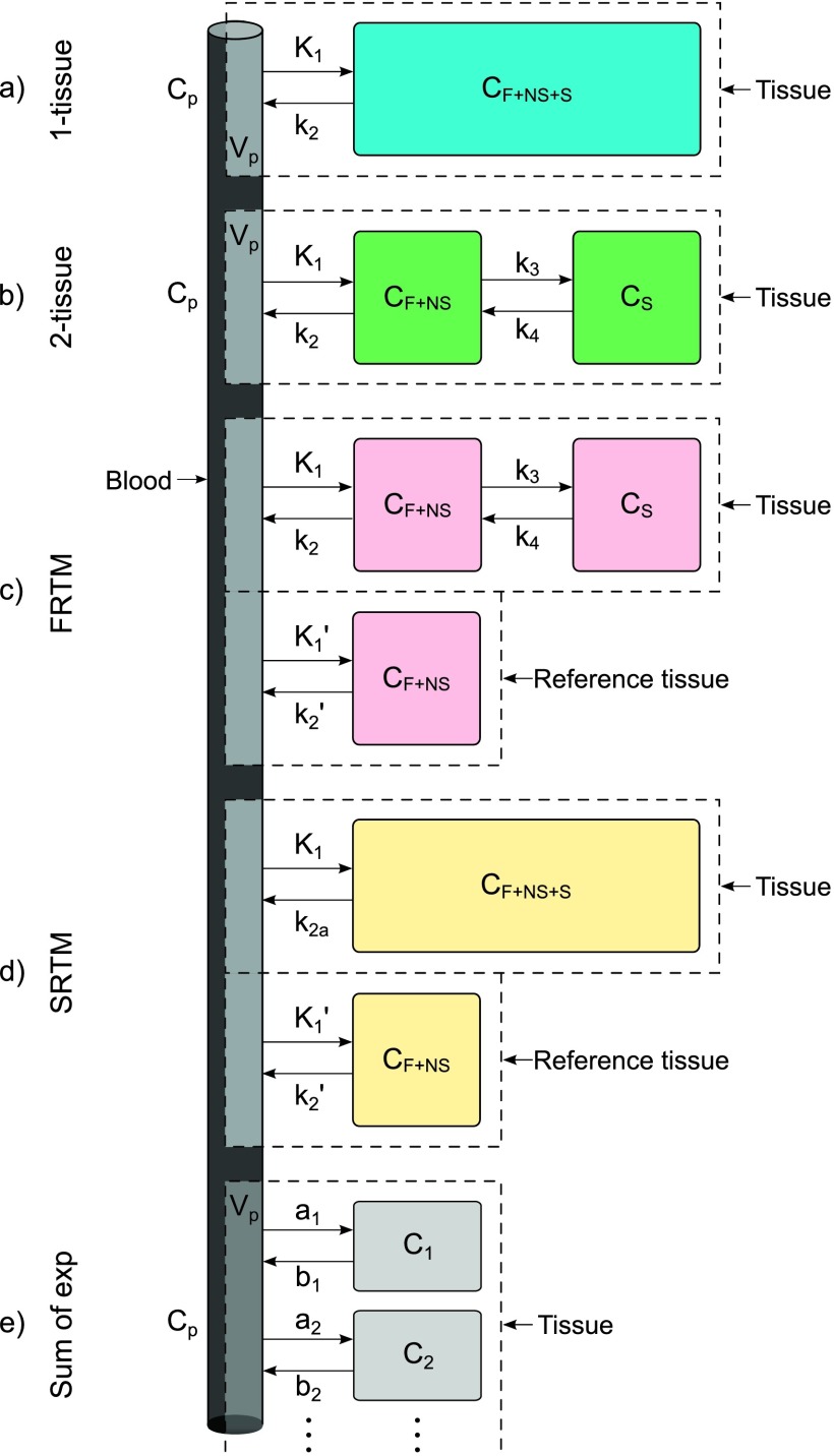
There are numerous models with different numbers of compartments described in the literature. These should be selected based on the particular tracer in question and limiting the number of parameters as the data allow. Common examples are the use of a 1-tissue compartment model for ¹⁵O-water or a 2-tissue model for ¹⁸F-FDG.²⁷ The models currently implemented in dynamic petstep (dpetstep) are shown in Fig. 1, where the denotation is F for free, NS for nonspecific, and S for specifically bound tracer in tissue.²⁸ The k’s are rate constants describing the rate of tracer exchange between the compartments, V_p is the fraction of arterial plasma appearing in tissue, and C_p is the tracer activity concentration in arterial plasma. The measured signal C_PET will be the sum of the comprising compartments. The blood volume is accounted for by a spillover term governed by V_p,²⁹

$${\displaystyle C_{\text{PET},p}=\left(1-V_p\right)C_{\text{PET}}+V_p{C}_p.}$$ (1)

If V_p is nonzero, Eqs. (2), (3), and (9) will include spillover according to Eq. (1).

FIG. 1.

Kinetic models implemented in dpetstep: (a) 1-tissue model, (b) 2-tissue model, (c) full reference tissue compartment model (FRTM), (d) simplified reference tissue model (SRTM), and (e) general sum of exponentials model. F = free tracer, NS = nonspecifically bound tracer, S = specifically bound tracer, p = arterial plasma.

2.A.1. 1-tissue model

The 1-tissue model is depicted in Fig. 1(a). The solution to the measured PET signal in tissue is³⁰

$${\displaystyle C_{\text{PET}}=K_1{e}^{-k_{2}t}*C_p,}$$ (2)

where “*” denotes temporal convolution.

2.A.2. 2-tissue model

Depicted in Fig. 1(b), the solution to the PET signal is³⁰

$${\displaystyle C_{\text{PET}}=\frac{K_1}{{\alpha }_2-{\alpha }_1}[(k_3+k_4-{\alpha }_1)e^{-{\alpha }_{1}t}+\hspace{0.17em}({\alpha }_2-k_3-k_4)e^{-{\alpha }_{2}t}]*C_p,}$$ (3)

where

$${\displaystyle {\alpha }_{1,2}=\frac{k_2+k_3+k_4\mp \sqrt{{(k_2+k_3+k_4)}^2-4k_2{k}_4}}{2}.}$$ (4)

The macroparameter referred to as the influx rate constant or metabolic flux constant K_i is calculated as³¹

$${\displaystyle K_i=\frac{K_1{k}_3}{k_2+k_3}.}$$ (5)

2.A.3. Full reference tissue compartment model (FRTM)

Reference tissue models are an alternative to using a known input function and instead use a reference region with no specific ligand binding. Figure 1(c) describes the FRTM.³² The constraints necessary for successful use of this model are:

• (i)The reference region should have no specific binding.
• (ii)The distribution volume in the tissue of interest equals that in the reference tissue ($K_1/k_2=K_1^{\prime }/k_2^{\prime }$).

The signal measured by the PET camera is³²

$${\displaystyle C_{\text{PET}}=R_1\left(C_{\text{ref}}+a{C}_{\text{ref}}*e^{-{\alpha }_{1}t}+b{C}_{\text{ref}}*e^{-{\alpha }_{2}t}\right),}$$ (6)

with

$${\displaystyle a=\frac{(k_3+k_4-{\alpha }_1)({\alpha }_1-k_2/R_1)}{\sqrt{{(k_2+k_3+k_4)}^2-4k_2{k}_4}},}$$

$${\displaystyle b=\frac{({\alpha }_2-k_3-k_4)({\alpha }_2-k_2/R_1)}{\sqrt{{(k_2+k_3+k_4)}^2-4k_2{k}_4}},}$$ (7)

where C_ref is the reference region TAC, α_1,2 are determined by Eq. (4), and the tracer delivery ratio $R_1=K_1/K_1^{\prime }=k_2/k_2^{\prime }$. The four fit parameters are R₁, k₂, k₃, and the binding potential BP_ND = k₃/k₄.

2.A.4. Simplified reference tissue model (SRTM)

The SRTM³³ in Fig. 1(d) is a development of the FRTM. Apart from the two constraints in FRTM, it has one further constraint that reduces the number of fit parameters from four to three:

• (iii)Specific and nonspecific compartments should be difficult to distinguish, i.e., the measured TAC can successfully be fitted to the 1-tissue model. Note that the two tissue compartments in FRTM [Fig. 1(c)] are approximated with a single tissue compartment in SRTM [Fig. 1(d)], with a new clearance rate constant $k_{2a}=k_2/\left(1+{\mathit{BP}}_{\text{ND}}\right)$.

The measured PET signal is calculated as³³

$${\displaystyle C_{\text{PET}}=R_1{C}_{\text{ref}}+\left(k_2-R_1{k}_{2a}\right)C_{\text{ref}}*e^{-k_{2a}t},}$$ (8)

with the three fit parameters R₁, k₂, and BP_ND.

2.A.5. Sum of exponentials

Also implemented in dpetstep is a very general kinetic model seen in Fig. 1(e), which comprises a sum of an arbitrary number of exponentials

$${\displaystyle C_{\text{PET}}=\sum _{i=1}^N{a}_i{e}^{-b_{i}t}*C_p,}$$ (9)

where the number of exponentials N is decided by the user, and the constants a and b are also set by the user.

2.B. Dynamic petstep

2.B.1. Simulation

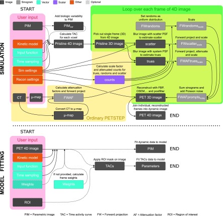
The petstep software takes a pristine input image and the corresponding CT image, adds effects of attenuation, random and scattered events, counting noise, system blurring, and then reconstructs it to produce a PET-like image.¹¹ In this paper we only briefly describe the major characteristics associated to petstep, and refer the reader to the original paper for more details. A schematic view of dpetstep is seen in Fig. 2. The items marked “*” in the list below indicate the process of petstep. The major steps of dpetstep are as follows:

• 1.The user inputs are: a parametric 4D image (3-spatial, 1-kinetic), the kinetic model, the desired time sampling scheme, an input function, a CT or μ-map of the object, and simulation and reconstruction settings (voxel sizes, average activity, etc.). The fourth parametric image dimension represents the model parameter.
• 2.Biologic variability can be added to the parametric image, in the form of Gaussian noise of the model’s parameters with standard deviation (SD) proportional to the parameter values. The noise model and SD proportionally constant can be adjusted by the user.
• 3.Identical TAC recalculation is avoided by checking the uniqueness of the parametric image voxels. Each set of unique voxels is calculated only once, e.g., an image containing ten different kinetic regions requires only ten TAC calculations, regardless of image matrix size.
  • 3.1.
    The TACs of each unique voxel are calculated using the user specified kinetic model, input function, and time sampling, according to Eqs. (2) and (3), or (9) [with or w/o Eq. (1)], or Eq. (6), or (8). The input function and time vectors are first upsampled to small equidistant vectors according to a user defined time step dt and interpolation method (default linear). The TACs are convolved and then interpolated back to the user set time sampling.
  • 3.2.
    Physical decay can be simulated according to the specified nuclide halflife. Decay factors for the ith frame are calculated as

    $${\displaystyle d_i=\frac{e^{-\lambda t_{i,\text{start}}}-e^{-\lambda t_{i,\text{end}}}}{\lambda \mathrm{\Delta }{t}_i},}$$ (10)

    where Δt_i is the frame duration, λ is the decay constant, t_i,start the start, and t_i,end the end time of the frame. Calculated TACs are multiplied by the decay factors.
• 4*.If the user supplied a CT of the object (Hounsfield units), it is converted to the corresponding linear attenuation coefficient map (μ-map, unit cm⁻¹) for PET photons. The μ-map is blurred by the system’s point spread function (PSF) and converted to forward projected attenuation factors (FWAF).
• 5.A conventional petstep simulation is performed sequentially on each frame (3D image) of the calculated pristine dynamic (4D) image.
  • 5.1*.
    The pristine 3D image is blurred with the imaging system’s PSF to mimic the effect of a real PET system, and forward projected to produce noise-free sinogram data.
  • 5.2*.
    The user specified scatter fraction (SF) and random fraction (RF) are used to properly scale the scatter and random counts (see the Appendix of the petstep paper¹¹).
  • 5.3*.
    The forward projected trues sinogram is attenuated by the calculated factors FWAF. The sinogram counts are scaled according to user set values. The triangular axial sensitivity is taken into account (lower counts toward end slices).
  • 5.4*.
    The attenuated true, random, and scatter sinograms are added to form a prompt sinogram, to which Poisson counting noise is included.
  • 5.5*.
    The noisy realizations of the sinogram data are reconstructed by FBP, OSEM, or OSEM with PSF correction, with optional postfiltering.
• 6.If physical decay was simulated, each reconstructed frame is decay corrected by multiplication with the inverse of the decay factor in Eq. (10).
• 7.The individually reconstructed frames are joined to form a single dynamic PET image.

FIG. 2.

Flowchart of the major steps of the simulation and model fitting processes in dpetstep.

2.B.2. Model fitting

After simulating a realistic dynamic PET data set with dpetstep, the data can be used with any external model fitting tool, such as the previously mentioned pmod. To simplify the use of dpetstep, we also included a basic fitting option however. The user can fit the data to a kinetic model either on an ROI basis, or voxel-wise to obtain parametric images. Weighted nonlinear least squares (WNLS) is used to fit image TACs to the chosen model. Below are the model fitting steps:

• 1.The user inputs a 4D PET image, kinetic model, input function, time sampling, initial guess, and optionally also an ROI mask. Lower and upper bounds for the estimates can be specified (default all zeros and 100 times the initial guess, respectively), and desired solver algorithm (default trust-region-reflective, see the matlab documentation for available solvers).
• 2.
  Frame weights are either provided by the user or calculated according to a model. Available models are:

  $${\displaystyle w_{1,i}=1,}$$

  $${\displaystyle w_{2,i}=\frac{1}{s^2},}$$

  $${\displaystyle w_{3,i}=d_i^2,}$$

  $${\displaystyle w_{4,i}=\frac{d_i}{\mathrm{\Delta }{t}_i{C}_i},}$$

  $${\displaystyle w_{5,i}=\frac{\mathrm{\Delta }{t}_i{e}^{-\lambda t_i}}{C_i},}$$

  $${\displaystyle w_{6,i}=\mathrm{\Delta }{t}_i{e}^{-\lambda t_i},}$$ (11)

  where i denotes frame number, t_i is the midframe time, s² the estimated (or known) frame variance, C_i the TAC value, and d_i the decay factor of the frame given by Eq. (10). The calculated weight vector is finally normalized to one.
• 3.The dynamic data, input function, and weight vectors are upsampled via linear interpolation to a small equidistant sampling dt, determined as the smallest time step in the provided time sampling. TAC values earlier than the first data time point are set to zero. Interpolated data time points that precisely overlap the original points retain the value of the original data point’s weight. For noncoincidental interpolated points, the weights are linearly interpolated by the surrounding original points.
• 4.The upsampled 4D data are WNLS fitted according Eqs. (2) and (3), or (9) [with or w/o Eq. (1)], or Eq. (6) or (8), with calculated or supplied weights. The result is one parameter set per ROI or per voxel (parametric image).

2.C. Simulation experiments

2.C.1. Monte Carlo simulation

The MC software gate (geant4 Application for Tomographic Emission, v5.0)³⁴ was used to perform 15 replicates of a complete dynamic 3D brain PET scan with a previously validated³⁵ GE Discovery LS PET (DLS) camera (18 detection rings, 672 BGO crystals per ring, crystal size 4 × 8 × 30 mm, transaxial FOV 550 mm, axial FOV 152 mm).

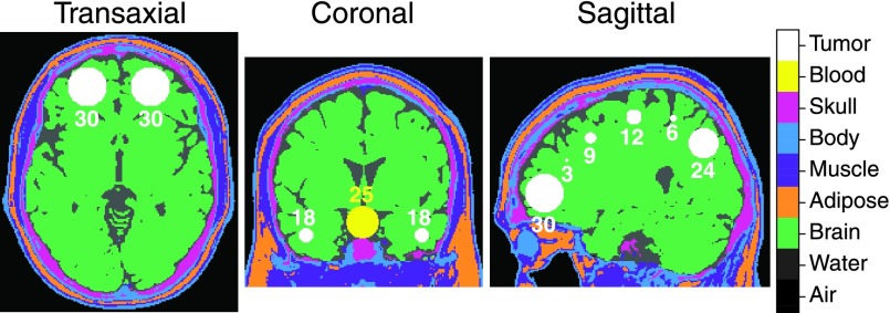
The digital BrainWeb head phantom³⁶ was used, and since we have described TAC generation and dynamic gate simulations with this phantom in previous studies,^26,37 they will only briefly be described here. The phantom consisted of nine materials as presented in Fig. 3, with seven homogenous spherical tumors of diameters from 3 to 30 mm distributed in both the right and left hemisphere (14 tumors in total), and a central 25 mm spherical blood region. The blood region was assigned a realistic input function C_p which was generated using matlab (v.8.1.0, The MathWorks, Inc., MA, USA). All other tissues in the head were also assigned realistic tissue TACs (TTACs) C_PET, generated according to the 2-tissue model. Specifically, the TTAC applied to all tumor regions was generated with realistic parameters for gliomas studied with ¹⁸F-FLT PET.³⁸ The values are seen in Table I. This noiseless, nondecayed 4D image set will be referred to as TRUE.

FIG. 3.

The voxelized brain phantom used in the simulations, consisting of nine regions with realistic TACs. Specifically, the blood region was assigned the input function C_p and all tumor regions were each assigned the same C_PET. The spherical regions are labeled with their respective diameter in mm.

TABLE I.

Kinetic parameter values of inserted tumors (Ref. 38).

K1	k2	k3	k4	Vp	Kia
(ml ⋅ g−1 ⋅ min−1)	(min−1)	(min−1)	(min−1)	(ml⋅g−1)	(ml ⋅ g−1 ⋅ min−1)
0.071	0.091	0.047	0.018	0.086	0.024

^aValue calculated by Eq. (5).

Fifteen simulation replicates of the setup were performed with a PET acquisition time of 60 min. Obtained true counts, SF, and RF are seen in Table II.

TABLE II.

Values obtained from the MC simulation and used as input in dpetstep, plus shared reconstruction settings.

Item	Value
True counts	0–7 ⋅ 106/frame
SF	0.289
RF	0.020
Radial bins	283
Projection angles	336
OSEM iterations	5
OSEM subsets	12
Postfilter XY	6 mm Gaussian
Postfilter Z	[1 2 1]/4
Frames	6 × 5 s, 3 × 10 s, 3 × 20 s, 2 × 30 s,
	2 × 60 s, 2 × 150 s, 10 × 300 s
Reconstructed matrix	165 × 165 × 35
Reconstructed voxel size	2 × 2 × 4.25 mm

One previous gate simulation data set for normalization and one for calibration were also used, as described in previous publications.^26,37

2.C.1.a. Image reconstruction.

The list-mode true+scattered coincidences from gate were binned into 3D sinograms³⁵ and reconstructed using one-step-late OSEM as implemented in stir (v.2.1).²⁵ Reconstruction settings and postfilter are seen in Table II. The OSEM settings were chosen to make sure that the tumor ROI values had converged, and corrections were made for normalization, decay, attenuation, and scatter.

For the AC, the BrainWeb phantom was converted to a μ-map for 511 keV photons in the respective phantom materials. The normalization sinogram was created from the normalization simulation data which were binned into a sinogram,¹¹ and the scatter estimation sinogram was created in stir, using the implemented SSS algorithm.

The dynamic PET data were reconstructed into dynamic image sets with 28 frames according to Table II, making a total of 60 min, and all images were finally calibrated to Bq ⋅ ml^-1.

2.C.2. dpetstep simulation

Fifteen replicates of the dynamic PET scan performed in gate were simulated in dpetstep according to the steps described in Sec. 2.B.1. The phantom used as a dynamic image input in gate (Fig. 3) was used as the corresponding parametric image input in dpetstep, resulting in the intermediate pristine image TRUE with decay. The phantom’s transaxial dimensions were padded with zeros to make it a square 331 × 331 matrix (resulting in a reconstructed 165 × 165 matrix with 2 × 2 mm voxels). The axial dimension was resampled from a 175 (slice width 1 mm) to a 35 matrix (slice width 4.25 mm), according to the DLS axial sampling.

The μ-map used in stir was used in dpetstep for attenuation and its correction. Simulation and reconstruction settings were set to the same as the MC simulation (Table II) with a few additional settings seen in Table III according to the measured DLS camera properties.³⁵ Note that the reported camera sensitivity was 6.44 cps ⋅ kBq⁻¹ ⋅ ml, for a maximum allowed ring difference of 18 (324 2D sinograms). Here we used a maximum ring difference of 11 (265 2D sinograms), decreasing the sensitivity to 6.44 ⋅ 265/324 = 5.27 cps ⋅ kBq⁻¹ ⋅ ml.

TABLE III.

Additional settings for dpetstep (Ref. 35).

Item	Value
Sensitivity	5.27 cps ⋅ kBq−1 ⋅ ml
PSF	5.1 mm
dt (convolution time step)	0.5 s

2.C.3. Plain TAC simulation

As mentioned in the Introduction, a common way to simulate dynamic PET is by simply adding Gaussian noise to a pristine TAC, or adding Poisson noise to a pristine sinogram. As a test of the added value of dpetstep compared to the plain TAC approach, 15 replicates of Gaussian-noised dynamic images were simulated. Each voxel TAC C^∗ of TRUE was Gaussian-noised individually by adding the noise distribution η to C^∗,³⁹

$${\displaystyle {\eta }_i=S\cdot rand\cdot \sqrt{\frac{C_i^{\ast }{e}^{-\lambda t_i}}{\mathrm{\Delta }{t}_i}},}$$

$${\displaystyle C_i=C_i^{\ast }+e^{\lambda t_i}{\eta }_i.}$$ (12)

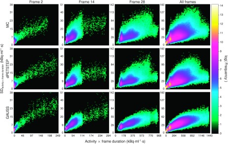
The variable rand is a random number from a Gaussian distribution with zero mean and variance equal to one. The scale factor S determines the magnitude of the noise, and was here set to 370. The value was found by first doing a coarse estimate of suitable noise level by visual inspection of the images and noise properties, followed by stepping it from 320 to 430 in steps of 10. The histogram of noise properties (Sec. 3, Fig. 8) was compared by the root mean squared error (RMSE). The scale factor was chosen to yield the minimum RMSE between the GAUSS and MC histograms. Again, 15 replicates were simulated and the individually noised TACs were joined to dynamic images which were postfiltered like all other simulations. The set will be referred to as GAUSS.

FIG. 8.

Logarithmic 2D histograms of scatter plots of voxel SD vs average activity (across 15 replicates), for early, middle, last, and all frames of all voxels of reconstructed images. Top row: MC, middle row: dpetstep, bottom row: GAUSS.

2.D. Kinetic parameter estimation

For both the MC as well as the dpetstep simulations, the input function C_p was image-derived from a spherical, 25 mm diameter ROI covering the true blood region. TTACs were derived from each voxel of the dynamic image. Kinetic parameters were estimated by WNLS fitting of each of the TTACs to the compartment model as implemented in dpetstep (Sec. 2.B.2), with frame weights w₆ according to Eq. (11).⁴⁰ All five kinetic parameters values were initialized as 0.01, for both MC and dpetstep. K_i was calculated according to Eq. (5).

2.E. Evaluating simulations

For all analyses, the zero background was masked off and omitted, as well as three end slices due to known end slice issues in stir (stir user’s guide v.2.1). The RMSE of the ith frame for the MC, dpetstep or GAUSS simulations, compared to TRUE, are calculated as

$${\displaystyle {\text{RMSE}}_i=\sqrt{\frac{{\displaystyle \sum _{j=1}^n{\left({\text{SIM}}_{i,j}-{\text{TRUE}}_{i,j}\right)}^2}}{{\displaystyle n}}},}$$ (13)

where SIM is the replicate average of the simulated data, j is the voxel, and n is the total number of voxels studied.

Normalized difference maps D are calculated as

$${\displaystyle D_{i,j}=\frac{\left({\text{SIM}}_{i,j}-{\text{REF}}_{i,j}\right)}{{\text{REF}}_{i,j}},}$$ (14)

where REF is any reference image, here either TRUE or the average (15 replicates) of the MC data. The nonparametric two-sample Kolmogorov–Smirnov (KS) test⁴¹ can be used to compare two sampled histograms of unknown distributions. It uses a measure of the distance between the two histograms to reject or keep the null hypothesis that the samples come from the same distribution, depending on how different they are in shape and location.

3. RESULTS

The time required to perform 15 replicate dpetstep simulations of the 331 × 331 × 35-sized input parametric image of size 1 × 1 × 4.25 mm, 28 frames, was 36 min (of which 1.4 s for the pristine 4D image calculation, and 19 s overhead time) on ten 2.9 GHz CPUs with the settings shown in Table II. For a single replicate, this corresponds to roughly 24 min/core computation time. In contrast, one replicate of the gate MC simulation required about 3300 h/core on the computer cluster Akka (Intel Xeon quad-core L5420 CPUs), HPC2N collaboration, Umeå University.

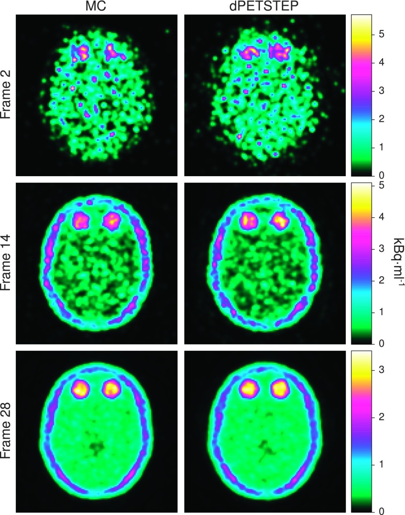
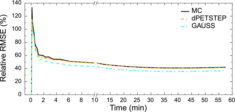
The reconstructed frame numbers 2, 14, and 28 of 28 (early at 5–10 s, middle at 2.5–3 min, and last at 55–60 min) from one of the 15 MC and dpetstep simulations are seen in Fig. 4. The relative RMSE per frame calculated by Eq. (13) is shown in Fig. 5. As seen, the RMSE of dpetstep conforms better with MC compared to GAUSS, indicating more similar noise properties. The frame average RMSE of dpetstep images was within 4% of the MC images, while the RMSE of GAUSS images was within 11% of MC.

FIG. 4.

Reconstructed early, middle, and last frame from both MC (left column) and dpetstep (right column) simulations.

FIG. 5.

RMSE relative TRUE of all frames of the three simulation sets.

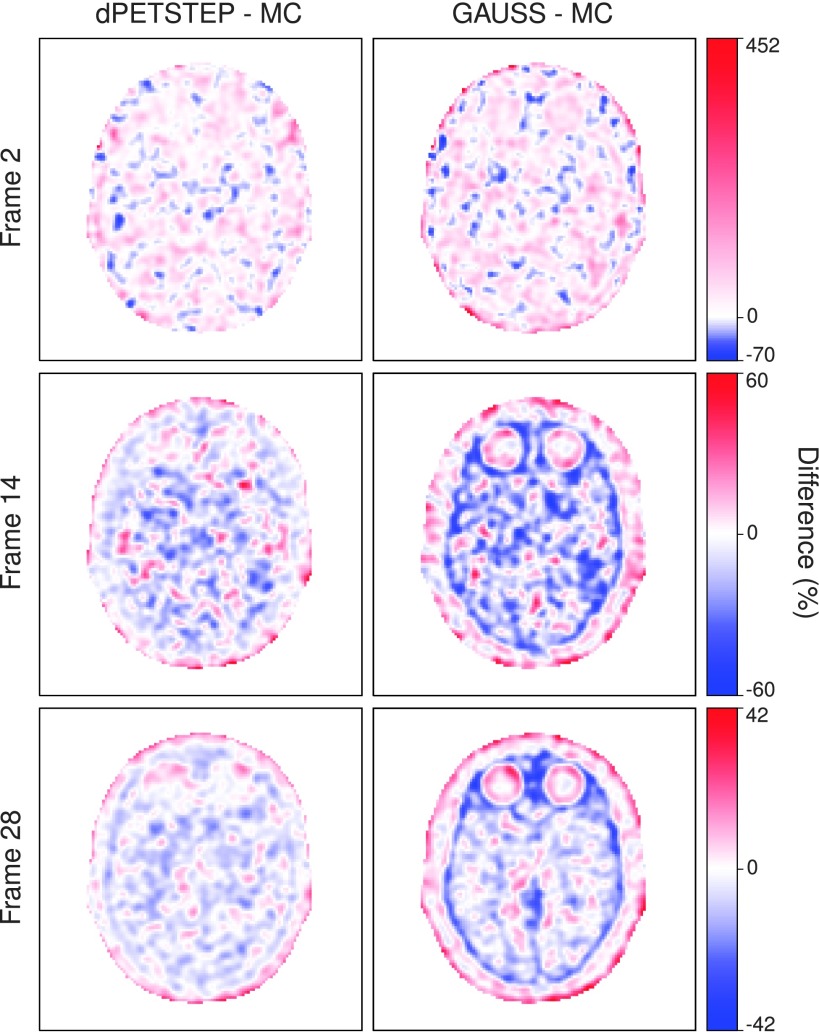
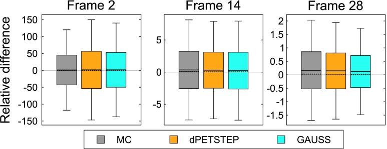
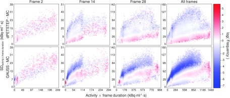
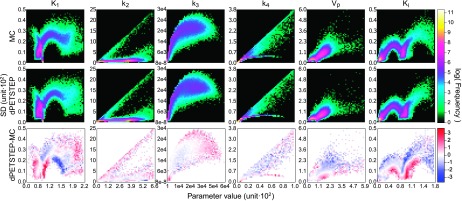
Difference maps by Eq. (14) of dpetstep and GAUSS relative MC are shown in Fig. 6. As can be seen for dpetstep, the differences appear to be mostly homogeneously noisy throughout the phantom, increasing somewhat toward the edge. For GAUSS, the difference map is less homogenous and shows more traces of the underlying image structures. Figure 7 shows the relative differences between the estimated values and the TRUE values [Eq. (14)] for all voxels of the 2nd, 14th, and 28th frame. The average relative difference over all frames was 24%, 24%, and 21% for MC, dpetstep, and GAUSS, respectively. All three medians were zero. Thus, the bias in dpetstep images matched that of MC, whereas GAUSS differed by 3% points. The image noise profile in dpetstep images compared to MC images was very similar, which can be seen in the scatter plot histograms of Fig. 8, where 2D histograms (size 50 × 50) of the voxel SD are shown as a function of voxel mean value for the three frames, as well as all frames (0–60 min). The SD and mean were calculated across the 15 simulation replicates. The histogram differences between MC and dpetstep and MC and GAUSS are seen in Fig. 9. The properties of the noise in dpetstep appear very similar to those found in the MC images. It was found that the noise profiles of GAUSS deviated more noticeably from the MC simulation, as can clearly be seen in Fig. 9. Similarly to the dynamic image analysis, Fig. 10 depicts the noise profiles in fitted parametric images, where data outside the 1st–99th percentile were omitted to keep the histograms more dense.

FIG. 6.

Difference maps for early, middle, and last frame, relative the respective MC images.

FIG. 7.

Differences relative TRUE for three frames. Boxes represent one SD, whiskers the 25^th and 75^th percentile, the full line is the mean, and the dashed line the median.

FIG. 9.

Logarithmic 2D histogram difference of voxel SD vs average activity (across 15 replicates), for early, middle, last, and all frames of all voxels of reconstructed images. Top row: dpetstep-MC, bottom row: GAUSS-MC.

FIG. 10.

Logarithmic 2D histograms of scatter plot of voxel SD vs mean value (across 15 replicates) of parametric images from both MC and dpetstep simulations. Parameter units are found in Table I. Top row: MC, middle row: dpetstep, bottom row: dpetstep-MC.

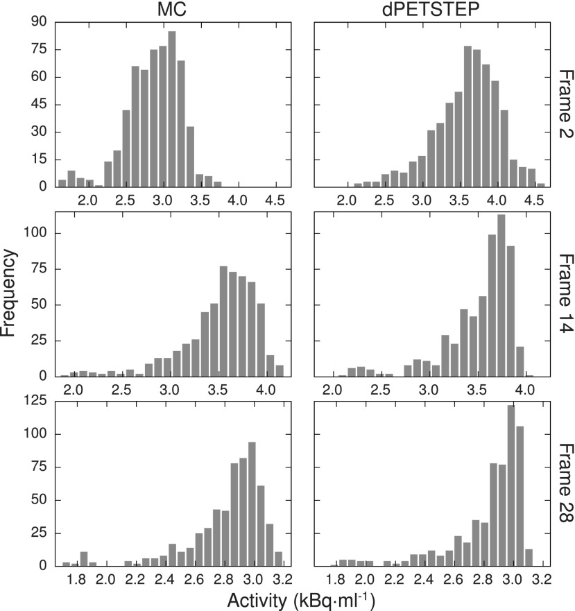
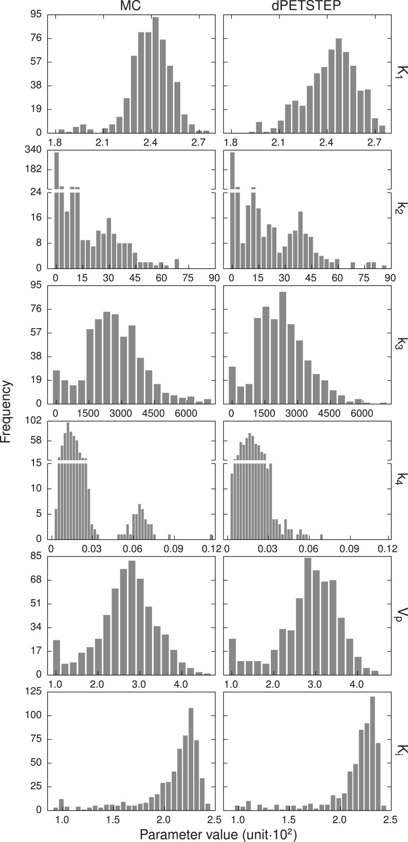
Figure 11 shows the average (across the 15 replicates) histograms of an ROI covering the largest two 30 mm tumors, for both MC and dpetstep, indicating similar noise profiles. The ROI was eroded by three voxels to avoid regions with high partial volume effects. The optimal number of bins used was calculated using the Freedman–Diaconis rule.⁴² Comparisons of the dpetstep to the MC histograms using the KS test concluded that they did not differ significantly for any frame (p < 0.01). Figure 12 shows the tumor ROI histograms of parametric images with optimal number of bins. Again, KS tests for the six histogram pairs found no significant differences between dpetstep and MC (p < 0.01).

FIG. 11.

Average tumor ROI histogram for three different frames (early, middle, and last) for MC (left column) and dpetstep (right column).

FIG. 12.

Average tumor ROI histograms for the six kinetic parameters for MC (left column) and dpetstep (right column). Parameter units are found in Table I.

The fitting implemented in dpetstep was verified against pmod, where simulated tumor ROI data were also fitted, using the same input. The fitted parameters agreed well despite using different estimators with resulting parameter estimates that were within each other’s error bars (figures not shown). Furthermore, the solving of the model equations was verified by saam II, where the same input generated consistent TACs for dpetstep and saam II within round-off errors (figures not shown).

4. DISCUSSION

As we have shown, both by tumor ROI histograms and as well as voxel-wise scatter plot histograms, image noise properties originating from dpetstep are very similar to those obtained from MC simulations. Going one step further and fitting the data to a compartment model also yields very similar results to MC.

The total computation time of dpetstep was around 24 min/core (per replicate), compared to the equivalent MC simulation requiring about 3300 h/core (excluding the reconstruction time of another couple of hours). dpetstep is thus more than 8000 times faster. One further note on timing is that OSEM takes more time compared to FBP. The same dpetstep simulation with FBP instead of OSEM required less than 3 min/core per replicate (results not presented). However, we emphasize that dpetstep uses simplified approximations of camera system properties, scatters, randoms, etc., and does not feature true photon transport. As a result, dpetstep is appropriate only when these details or a high level of accuracy are unnecessary. Furthermore, neither petstep nor dpetstep simulates full 3D data. This is accounted for by adjusting the number of counts from the 2D projection data to obtain similar noise equivalent counts as measured in 3D. However, slice correlations found in real PET data are not present in dpetstep data. This effect is however very reduced in real data when applying axial postfiltering.

The obtained noise properties (Fig. 8) indicate that the Gaussian approach yields results that deviate, at times to a rather large extent, from MC. Furthermore, the difference maps between any simulation method and MC should ideally be uniformly noisy, indicating that all regions of the phantom, regardless of level of uptake and location, get realistic noise and uptake properties and hence are unbiased. The difference maps clearly show that GAUSS results in images that are more biased compared to dpetstep. The differences are more noticeably dependent on the underlying object structures, meaning that although the total RMSE or other measures of the total image results may be rather good, the bias and noise can differ a lot throughout the image. For example, the simulated image can have realistic properties in one region of the phantom, and rather unrealistic in another. It is worth noting again that all images have been postfiltered by the same filter. A smaller transaxial filter than the 6 mm used here would likely result in difference maps with even more pronounced underlying structures showing, since there would be less smearing of the image.

The differences from TRUE were on average nonzero (Fig. 7), implying that the simulation plus reconstruction process introduces bias. The bias throughout the frames is of similar shape and size for dpetstep and GAUSS as MC however, indicating that the introduced bias is realistic and expected. Postfiltering followed by background masking discarded some individual voxels which caused a small bias, and the nonnegativity constraint for all images also introduces bias. We thus present Fig. 6 relative MC and not TRUE, because we are interested in producing PET-like images that include realistic adverse effects (i.e., count noise, resolution loss, etc., as found in MC) rather than unrealistic ideal images (i.e., TRUE).

The Gaussian approach did not produce as realistic noise properties as dpetstep, which should be taken into consideration when deciding on simulation method for the intended use. The computation time for GAUSS was about 7 s/core however, compared to the dpetstep simulation which required about 24 min/core (per replicate).

Some peculiar patterns were found in the parametric image scatter plots in Fig. 10. It is reassuring, however, that odd clusters are visible in both the MC and dpetstep simulations. When studying the absolute parameter values in the histograms of Fig. 12, one notices that some values are rather far from the true values (Table I). The parameter estimations are sensitive to the initial guesses, frame weights, fitting method, constraints, and more. Here we used start guesses of 0.01 for all parameters. Other guesses could likely result in better estimations. Moreover, since the parameters are correlated, heavy over/underestimation of one parameter coupled with another being largely over/underestimated, may still produce an overall good fit. The aim of this study was not to develop/evaluate fitting algorithms or use the estimates, but to evaluate the properties of simulated dpetstep images. Thus, the values of parameter estimates were not of interest and not investigated.

Although only five kinetic models are currently implemented in dpetstep, addition of more models is easy due to the modular nature of the dpetstep code. We also note that the sum of exponentials model [Eq. (9)] can be used to represent a vast range of kinetic models, by appropriate translation of model parameters.

There are many sources of uncertainty and bias that complicate the estimation of the “true” kinetic parameters of a tumor and its surrounding tissue. These can be roughly broken down by origin into physical and biological sources of uncertainty. A few of the more prevalent examples of physical origin are spatial data sampling (i.e., partial volume effect, temporal data sampling, injected activity, and data postprocessing, such as image reconstruction and tracer kinetics model selection. Examples of biological origin are tumor heterogeneity (i.e., the length scale of the variation of the tumor’s uptake), nonspecific uptake, involuntary patient motion, abnormal or variable patient physiology and metabolism, receptor saturation, and tracer binding/stability. To reduce the uncertainty of the estimates of the kinetics parameters the researcher has some control over the data acquisition process. For example, the data sampling, image reconstruction, compartment model, and fitting strategies can be altered to improve (or worsen) the parameter estimates.⁴³ However, the judicious choice of these parameters often requires knowledge of that same underlying biology that they are seeking to estimate. To put it simply, it is the modeler’s job to choose these parameters that best reduce the uncertainty and bias of the final estimates. A tool like dpetstep can be a great aid when tackling these questions. A tool such as dpetstep allows researchers to investigate both physical and biological phenomena such as those mentioned above, and their effect on dynamic and parametric PET images. Furthermore, dpetstep could also be useful in fields such as dosimetry for improved dose estimation from new tracers, and in system performance evaluation to help in study design.

5. CONCLUSION

We have demonstrated that dpetstep is able to simulate realistic 4D PET scans in a fraction of the time taken with a commonly used MC tool, where noise properties in both the dynamic images and subsequent parametric images conform very well to MC data.

We believe dpetstep to be very useful for purposes requiring fast, simple, and realistic results but are less dependent on highly accurate scatter and random events representation. This tool is a one-stop solution offering all tools necessary for complete dynamic PET simulations including solving model equations, system response, count noise, scatters and randoms, image reconstruction methods, and parameter/parametric image estimation. dpetstep can be downloaded for no cost from https://github.com/CRossSchmidtlein/dPETSTEP.

CONFLICT OF INTEREST DISCLOSURE

The authors report no conflict of interest regarding this work.

REFERENCES

- 1.Muzi M., O’Sullivan F., Mankoff D. A., Doot R. K., Pierce L. A., Kurland B. F., Linden H. M., and Kinahan P. E., “Quantitative assessment of dynamic PET imaging data in cancer imaging,” Magn. Reson. Imaging 30, 1203–1215 (2012). 10.1016/j.mri.2012.05.008 [DOI] [PMC free article] [PubMed] [Google Scholar]
- 2.Weber W. A., “Positron emission tomography as an imaging biomarker,” J. Clin. Oncol. 24, 3282–3292 (2006). 10.1200/JCO.2006.06.6068 [DOI] [PubMed] [Google Scholar]
- 3.Clarke L. P., Croft B. S., Nordstrom R., Zhang H., Kelloff G., and Tatum J., “Quantitative imaging for evaluation of response to cancer therapy,” Transl. Oncol. 2, 195–197 (2009). 10.1593/tlo.09217 [DOI] [PMC free article] [PubMed] [Google Scholar]
- 4.Häggström I., Johansson L., Larsson A., Östlund N., Sörensen J., and Karlsson M., “Semi-automatic tumour segmentation by selective navigation in a three-parameter volume, obtained by voxel-wise kinetic modelling of 11C-acetate,” Radiat. Prot. Dosim. 139, 214–218 (2010). 10.1093/rpd/ncq075 [DOI] [PubMed] [Google Scholar]
- 5.Sörensen J., “How does the patient benefit from clinical PET?,” Theranostics 2, 427–436 (2012). 10.7150/thno.3794 [DOI] [PMC free article] [PubMed] [Google Scholar]
- 6.Cheebsumon P., van Velden F. H. P., Yaqub M., Hoekstra C. J., Velasquez L. M., Hayes W., Hoekstra O. S., Lammertsma A. A., and Boellaard R., “Measurement of metabolic tumor volume: Static versus dynamic FDG scans,” EJNMMI Res. 1, 1–9 (2011). 10.1186/2191-219X-1-35 [DOI] [PMC free article] [PubMed] [Google Scholar]
- 7.Visser E. P., Philippens M. E. P., Kienhorst L., Kaanders J. H. A. M., Corstens F. H. M., de Geus-Oei L.-F., and Oyen W. J. G., “Comparison of tumor volumes derived from glucose metabolic rate maps and SUV maps in dynamic 18F-FDG PET,” J. Nucl. Med. 49, 892–898 (2008). 10.2967/jnumed.107.049585 [DOI] [PubMed] [Google Scholar]
- 8.Dimitrakopoulou-Strauss A., Strauss L. G., Schwarzbach M., Burger C., Heichel T., Willeke F., Mechtersheimer G., and Lehnert T., “Dynamic PET 18F-FDG studies in patients with primary and recurrent soft-tissue sarcomas: Impact on diagnosis and correlation with grading,” J. Nucl. Med. 42, 713–720 (2001). [PubMed] [Google Scholar]
- 9.Dimitrakopoulou-Strauss A., Strauss L. G., and Rudi J., “PET-FDG as predictor of therapy response in patients with colorectal carcinoma,” Q. J. Nucl. Med. 47, 8–13 (2003). [PubMed] [Google Scholar]
- 10.Muzi M., Vesselle H., Grierson J. R., Mankoff D. A., Schmidt R. A., Peterson L., Wells J. M., and Krohn K. A., “Kinetic analysis of 3’-deoxy-3’-fluorothymidine PET studies: Validation studies in patients with lung cancer,” J. Nucl. Med. 46, 274–282 (2005). [PubMed] [Google Scholar]
- 11.Berthon B., Häggström I., Apte A., Beattie B. J., Kirov A. S., Humm J. L., Marshall C., Spezi E., Larsson A., and Schmidtlein C. R., “ petstep: Generation of synthetic PET lesions for fast evaluation of segmentation methods,” Phys. Med. 31, 969–980 (2015). 10.1016/j.ejmp.2015.07.139 [DOI] [PMC free article] [PubMed] [Google Scholar]
- 12.Hudson H. M. and Larkin R. S., “Accelerated image reconstruction using ordered subsets of projection data,” IEEE Trans. Med. Imaging 13, 601–609 (1994). 10.1109/42.363108 [DOI] [PubMed] [Google Scholar]
- 13.Barrett H. H., Wilson D. W., and Tsui B. M. W., “Noise properties of the EM algorithm. I. Theory,” Phys. Med. Biol. 39, 833–846 (1994). 10.1088/0031-9155/39/5/004 [DOI] [PubMed] [Google Scholar]
- 14.Boellaard R., van Lingen A., and Lammertsma A. A., “Experimental and clinical evaluation of iterative reconstruction (OSEM) in dynamic PET: Quantitative characteristics and effects on kinetic modeling,” J. Nucl. Med. 42, 808–817 (2001). [PubMed] [Google Scholar]
- 15.Wilson D. W. and Tsui B. M. W., “Noise properties of filtered-backprojection and ML-EM reconstructed emission tomographic images,” IEEE Trans. Nucl. Sci. 40, 1198–1203 (1993). 10.1109/23.256736 [DOI] [Google Scholar]
- 16.Schmidtlein C. R., Beattie B. J., Bailey D. L., Akhurst T. J., Wang W., Gönen M., Kirov A. S., and Humm J. L., “Using an external gating signal to estimate noise in PET with an emphasis on tracer avid tumors,” Phys. Med. Biol. 55, 6299–6326 (2010). 10.1088/0031-9155/55/20/016 [DOI] [PubMed] [Google Scholar]
- 17.Qi J., “A unified noise analysis for iterative image estimation,” Phys. Med. Biol. 48, 3505–3519 (2003). 10.1088/0031-9155/48/21/004 [DOI] [PubMed] [Google Scholar]
- 18.Li Y., “Noise propagation for iterative penalized-likelihood image reconstruction based on Fisher information,” Phys. Med. Biol. 56, 1083–1103 (2011). 10.1088/0031-9155/56/4/013 [DOI] [PubMed] [Google Scholar]
- 19.Muzic R. F. and Cornelius S., “ comkat: Compartment model kinetic analysis tool,” J. Nucl. Med. 42, 636–645 (2001). [PubMed] [Google Scholar]
- 20.Karakatsanis N. A., Lodge M. A., Tahari A. K., Zhou Y., Wahl R. L., and Rahmim A., “Dynamic whole-body PET parametric imaging: I. Concept, acquisition protocol optimization and clinical application,” Phys. Med. Biol. 58, 7391–7418 (2013). 10.1088/0031-9155/58/20/7391 [DOI] [PMC free article] [PubMed] [Google Scholar]
- 21.Comtat C., Kinahan P. E., Defrise M., Michel C., Lartizien C., and Townsend D. W., “Simulating whole-body PET scanning with rapid analytical methods,” in IEEE Nuclear Science Symposium Medical Imaging Conference Record (IEEE, Seattle, WA, 1999), pp. 1260–1264. [Google Scholar]
- 22.Kotasidis F. A., Tsoumpas C., Polycarpou I., and Zaidi H., “A 5D anthropomorphic numerical phantom for parametric imaging simulation studies in dynamic emission tomography,” Comput. Med. Imaging Graphics 38, 764–773 (2014). 10.1016/j.compmedimag.2014.06.018 [DOI] [PubMed] [Google Scholar]
- 23.Wang G. and Qi J., “PET image reconstruction using kernel method,” IEEE Trans. Med. Imaging 34, 61–71 (2014). 10.1109/TMI.2014.2343916 [DOI] [PMC free article] [PubMed] [Google Scholar]
- 24.Karakatsanis N. A., Zhou Y., Lodge M. A., Casey M. E., Wahl R. L., Zaidi H., and Rahmim A., “Generalized whole-body Patlak parametric imaging for enhanced quantification in clinical PET,” Phys. Med. Biol. 60, 8643–8673 (2015). 10.1088/0031-9155/60/22/8643 [DOI] [PMC free article] [PubMed] [Google Scholar]
- 25.Thielemans K., Tsoumpas C., Mustafovic S., Beisel T., Aguiar P., Dikaios N., and Jacobson M. W., “ stir: Software for tomographic image reconstruction release 2,” Phys. Med. Biol. 57, 867–883 (2012). 10.1088/0031-9155/57/4/867 [DOI] [PubMed] [Google Scholar]
- 26.Häggström I., Schmidtlein C. R., Karlsson M., and Larsson A., “Compartment modeling of dynamic brain PET—The impact of scatter corrections on parameter errors,” Med. Phys. 41, 111907 (9pp.) (2014). 10.1118/1.4897610 [DOI] [PubMed] [Google Scholar]
- 27.Watabe H., Ikoma Y., Kimura Y., Naganawa M., and Shidahara M., “PET kinetic analysis—Compartmental model,” Ann. Nucl. Med. 20, 583–588 (2006). 10.1007/BF02984655 [DOI] [PubMed] [Google Scholar]
- 28.Innis R. B., Cunningham V. J., Delforge J., Fujita M., Gjedde A., Gunn R. N., Holden J., Houle S., Huang S.-C., Ichise M., Iida H., Ito H., Kimura Y., Koeppe R. A., Knudsen G. M., Knuuti J., Lammertsma A. A., Laruelle M., Logan J., Maguire R. P., Mintun M. A., Morris E. D., Parsey R., Price J. C., Slifstein M., Sossi V., Suhara T., Votaw J. R., Wong D. F., and Carson R. E., “Consensus nomenclature for in vivo imaging of reversibly binding radioligands,” J. Cereb. Blood Flow Metab. 27, 1533–1539 (2007). 10.1038/sj.jcbfm.9600493 [DOI] [PubMed] [Google Scholar]
- 29.Lodge M. A., Carson R. E., Carrasquillo J. A., Whatley M., Libutti S. K., and Bacharach S. L., “Parametric images of blood flow in oncology PET studies using [15O] water,” J. Nucl. Med. 41, 1784–1792 (2000). [PubMed] [Google Scholar]
- 30.Kamasak M. E., “Computation of variance in compartment model parameter estimates from dynamic PET data,” Med. Phys. 39, 2638–2648 (2012). 10.1118/1.3702456 [DOI] [PubMed] [Google Scholar]
- 31.Schiepers C., Chen W., Dahlbom M., Cloughesy T. F., Hoh C. K., and Huang S.-C., “18F-fluorothymidine kinetics of malignant brain tumors,” Eur. J. Nucl. Med. Mol. Imaging 34, 1003–1011 (2007). 10.1007/s00259-006-0354-5 [DOI] [PubMed] [Google Scholar]
- 32.Lammertsma A. A., Bench C. J., Hume S. P., Osman S., Gunn K., Brooks D. J., and Frackowiak R. S., “Comparison of methods for analysis of clinical [11C]raclopride studies,” J. Cereb. Blood Flow Metab. 16, 42–52 (1996). 10.1097/00004647-199601000-00005 [DOI] [PubMed] [Google Scholar]
- 33.Lammertsma A. A. and Hume S. P., “Simplified reference tissue model for PET receptor studies,” Neuroimage 4, 153–158 (1996). 10.1006/nimg.1996.0066 [DOI] [PubMed] [Google Scholar]
- 34.Jan S., Santin G., Strul D., Staelens S., Assié K., Autret D., Avner S., Barbier R., Bardiès M., Bloomfield P. M., Brasse D., Breton V., Bruyndonckx P., Buvat I., Chatziioannou A. F., Choi Y., Chung Y. H., Comtat C., Donnarieix D., Ferrer L., Glick S. J., Groiselle C. J., Guez D., Honore P.-F., Kerhoas-Cavata S., Kirov A. S., Kohli V., Koole M., Krieguer M., van der Laan D. J., Lamare F., Largeron G., Lartizien C., Lazaro D., Maas M. C., Maigne L., Mayet F., Melot F., Merheb C., Pennacchio E., Perez J., Pietrzyk U., Rannou F. R., Rey M., Schaart D. R., Schmidtlein C. R., Simon L., Song T. Y., Vieira J.-M., Visvikis D., de Walle R. V., Wieërs E., Morel C., and van de Walle R., “ gate: A simulation toolkit for PET and SPECT,” Phys. Med. Biol. 49, 4543–4561 (2004). 10.1088/0031-9155/49/19/007 [DOI] [PMC free article] [PubMed] [Google Scholar]
- 35.Schmidtlein C. R., Kirov A. S., Nehmeh S. A., Erdi Y. E., Humm J. L., Amols H. I., Bidaut L. M., Ganin A., Stearns C. W., McDaniel D. L., and Hamacher K. A., “Validation of gate Monte Carlo simulations of the GE Advance/Discovery LS PET scanners,” Med. Phys. 33, 198–208 (2006). 10.1118/1.2089447 [DOI] [PubMed] [Google Scholar]
- 36.Collins D. L., Zijdenbos A. P., Kollokian V., Sled J. G., Kabani N. J., Holmes C. J., and Evans A. C., “Design and construction of a realistic digital brain phantom,” IEEE Trans. Med. Imaging 17, 463–468 (1998). 10.1109/42.712135 [DOI] [PubMed] [Google Scholar]
- 37.Häggström I., Axelsson J., Schmidtlein C. R., Karlsson M., Garpebring A., Johansson L., Sörensen J., and Larsson A., “A Monte Carlo Study of the dependence of early frame sampling on uncertainty and bias in pharmacokinetic parameters from dynamic PET,” J. Nucl. Med. Technol. 43, 53–60 (2015). 10.2967/jnmt.114.141754 [DOI] [PubMed] [Google Scholar]
- 38.Schiepers C., Dahlbom M., Chen W., Cloughesy T. F., Czernin J., Phelps M. E., and Huang S.-C., “Kinetics of 3′-deoxy-3′-18F-fluorothymidine during treatment monitoring of recurrent high-grade glioma,” J. Nucl. Med. 51, 720–727 (2010). 10.2967/jnumed.109.068361 [DOI] [PubMed] [Google Scholar]
- 39.Logan J., Fowler J. S., Volkow N. D., Ding Y. S., Wang G. J., and Alexoff D. L., “A strategy for removing the bias in the graphical analysis method,” J. Cereb. Blood Flow Metab. 21, 307–320 (2001). 10.1097/00004647-200103000-00014 [DOI] [PubMed] [Google Scholar]
- 40.Thiele F. and Buchert R., “Evaluation of non-uniform weighting in non-linear regression for pharmacokinetic neuroreceptor modelling,” Nucl. Med. Commun. 29, 179–188 (2008). 10.1097/MNM.0b013e3282f28138 [DOI] [PubMed] [Google Scholar]
- 41.Massey F. J., “The Kolmogorov–Smirnov test for goodness of fit,” J. Am. Stat. Assoc. 46, 68–78 (1951). 10.1080/01621459.1951.10500769 [DOI] [Google Scholar]
- 42.Freedman D. and Diaconis P., “On the histogram as a density estimator: L2 theory,” Z. Wahrscheinlichkeitstheorie Verw. Geb. 57, 453–476 (1981). 10.1007/BF01025868 [DOI] [Google Scholar]
- 43.The use of agonists/antagonists and other forms of interventions such as anesthesia can also be used but are outside the bounds of this tool in its present form.