Segmentation of prostate from ultrasound images using level sets on active band and intensity variation across edges

Abstract

Purpose:

In this paper, the authors propose a novel efficient method to segment ultrasound images of the prostate with weak boundaries. Segmentation of the prostate from ultrasound images with weak boundaries widely exists in clinical applications. One of the most typical examples is the diagnosis and treatment of prostate cancer. Accurate segmentation of the prostate boundaries from ultrasound images plays an important role in many prostate-related applications such as the accurate placement of the biopsy needles, the assignment of the appropriate therapy in cancer treatment, and the measurement of the prostate volume.

Methods:

Ultrasound images of the prostate are usually corrupted with intensity inhomogeneities, weak boundaries, and unwanted edges, which make the segmentation of the prostate an inherently difficult task. Regarding to these difficulties, the authors introduce an active band term and an edge descriptor term in the modified level set energy functional. The active band term is to deal with intensity inhomogeneities and the edge descriptor term is to capture the weak boundaries or to rule out unwanted boundaries. The level set function of the proposed model is updated in a band region around the zero level set which the authors call it an active band. The active band restricts the authors’ method to utilize the local image information in a banded region around the prostate contour. Compared to traditional level set methods, the average intensities inside∖outside the zero level set are only computed in this banded region. Thus, only pixels in the active band have influence on the evolution of the level set. For weak boundaries, they are hard to be distinguished by human eyes, but in local patches in the band region around prostate boundaries, they are easier to be detected. The authors incorporate an edge descriptor to calculate the total intensity variation in a local patch paralleled to the normal direction of the zero level set, which can detect weak boundaries and avoid unwanted edges in the ultrasound images.

Results:

The efficiency of the proposed model is demonstrated by experiments on real 3D volume images and 2D ultrasound images and comparisons with other approaches. Validation results on real 3D TRUS prostate images show that the authors’ model can obtain a Dice similarity coefficient (DSC) of 94.03% ± 1.50% and a sensitivity of 93.16% ± 2.30%. Experiments on 100 typical 2D ultrasound images show that the authors’ method can obtain a sensitivity of 94.87% ± 1.85% and a DSC of 95.82% ± 2.23%. A reproducibility experiment is done to evaluate the robustness of the proposed model.

Conclusions:

As far as the authors know, prostate segmentation from ultrasound images with weak boundaries and unwanted edges is a difficult task. A novel method using level sets with active band and the intensity variation across edges is proposed in this paper. Extensive experimental results demonstrate that the proposed method is more efficient and accurate.

1. INTRODUCTION

In this paper, we propose a novel efficient method to segment ultrasound images of the prostate with weak boundaries. Accurate segmentation of the prostate from ultrasound images plays an important role in many prostate-related applications such as the accurate placement of the biopsy needles, the assignment of the appropriate therapy in cancer treatment, and the measurement of the prostate gland volume. Prostate cancer is the second most frequently diagnosed cancer (at 15% of all male cancers)¹ and the fifth most common cancer overall.² Ultrasound imaging is the main modality for prostate cancer diagnosis and treatment. For the purpose of prostate cancer diagnosis and image-guided surgical planning and therapy, segmentation of the prostate from 2D or 3D ultrasound images is challenged. Although segmentation can be done manually, it is time consuming and depends on the experience, skill, and technique of the radiologists. Computer-aided segmentation algorithms can reduce the inefficiency caused by manual segmentation. However, in ultrasound images, the contrast is low and the intensity is inhomogeneous. Also speckles and weak edges make the ultrasound images inherently difficult to be segmented. Segmentation of ultrasound prostate images becomes a challenging work which is mainly due to the following three characteristics of ultrasound prostate images. First, the signal-to-noise ratio is low, thus algorithms relying on the intensity of single pixel frequently fail to segment this kind of images. Second, prostate boundaries are usually weak and texture information between interior and exterior of prostates is similar. Therefore, most of the segmentation algorithms based on simple edge detector (e.g., canny edge detector) could not get satisfying segmentation results. Third, it is hard to get better segmentation results in apex and base slices when segmenting 3D TRUS images. Apex and base are the superior and inferior of a prostate. They are not always visible in TRUS images.

Prostate segmentation methods can be roughly divided into three categories: contour and shape based methods, region based methods, and classification based methods (supervised and unsupervised). Contour and shape based methods use contour and shape information to segment the prostate images. Nouranian et al.³ proposed a multiatlas based fusion framework to automatically delineate prostate boundaries in ultrasound images. A pairwise atlas agreement factor is introduced in the atlas selection stage. Ladak et al.⁴ used a discrete dynamic contour (DDC)⁵ model with four user selected points to segment the 2D prostate images. The position of a contour is represented by discrete points known as the vertices. The moving of the vertex points is guided by two forces: external force and internal force. External force is defined by image gradient and internal force restricts the smoothness of the contour. Although DDC is time saving, it fails to produce acceptable results in the areas where the prostate boundaries are missing. Jendoubi et al.⁶ used gradient vector flow as external force to drive the evolving contour toward the prostate boundary. Chiu et al.⁷ used Mallat’s multiscale edge detection method to calculate the image gradient and then utilized the image gradient as external force of the DDC model. Yan et al.^8,9 proposed a statistical shape model to learn the shape statistics from TRUS sequences. The learned shape statistics are then incorporated into a deformable contour model. The contour evolution is not only guided by internal and external forces but also by shape constraints derived from the shape statistics. In Ref. 10, a multiresolution based parametric deformable statistical model of shape and appearance is used to segment the prostate TRUS images. Local phase information is incorporated to build the statistical model. Kim and Seo¹¹ used Gabor texture features and snake-like contour to extract the prostate boundary. In Ref. 12, the authors proposed a variational formulation based on deformable super-ellipses and region energy based on the assumption of a Rayleigh distribution. However, in their model, there are seven super-ellipse parameters needed to be optimized which is time consuming and inconvenient.

Region based methods use local intensity or statistics like mean and standard deviation in the energy minimization frameworks. Ding et al.¹³ described a slice-based 3D prostate segmentation method based on a continuity constraint, implemented as an autoregressive model. Fan et al.¹⁴ proposed a region based level set framework to segment prostate contours from ultrasound images. Yu et al.¹⁵ proposed a slice-based method for 3D ultrasound image segmentation. The initial prostate boundaries are automatically determined by the radial bas-relief method. Then a region-based level set framework is applied to deform the initial contours. Finally, the segmented contours on initial frames are propagated to the adjacent frames as their initial contours until all the frames are segmented. In Ref. 16, Qiu et al. incorporated an inherent geometric/axial symmetry shape prior into a 3-D prostate segmentation model. A coherent continuous max-flow method is used to solve the segmentation model. In Ref. 17, the symmetry of prostate is incorporated into a level set framework for 3D end-firing TRUS segmentation. The segmentation result of one 2D-slice is propagated to assist in segmenting its surrounding slices. In Ref. 18, the authors built a coarse-to-fine graph partition scheme to segment the prostate from 2D ultrasound images. The initial contour obtained by graph cut segmentation is further refined in a fuzzy inference framework. The membership of a pixel is determined by the region statistics.

Classification based methods use a set of training data with labeled objects as prior information to build a predictor to assign labels to unlabeled observations. Zhan and Shen¹⁹ trained both a Gabor filter based support vector machine (G-SVM) and a 3D mean-shape model to obtain the texture and shape information in the images. For a new patient TRUS sequence, the prior information will guide a 3D deformable model to the prostate boundaries. Instead of using Gabor filter bank to extract the prostate feature, Akbari and Fei²⁰ used wavelet transform for prostate feature extraction. In Ref. 21, a 3D prostate US segmentation algorithm using patch-based anatomical features and support vector machines had been presented and has potential for extension to intrafraction motion estimation. Ghose et al.²² proposed an algorithm for automatic prostate segmentation that can be applicable for prostate brachytherapy. Their approach is based on three independent 2-D active shape and appearance models that are generated for central, apex, and base zones. There are many other algorithms for ultrasound image segmentation; more related studies can be found in Refs. ^23–28.

Various ultrasound prostate segmentation methods have been proposed in recent years. As we know, it is hard for existing algorithms to get satisfying segmentation results while segmenting images with weak boundaries and unwanted edges. Some of these methods are devoted to incorporate edge information to get promising segmentation results (Refs. ^{6, 7}, and ¹¹). However, due to the poor quality of ultrasound images, they are more sensitive to noise, intensity inhomogeneities, etc. The prostate contours obtained by those methods are often incomplete. In this paper, we introduce an active band term and an edge descriptor term in the modified level set energy functional. The active band term is to deal with intensity inhomogeneities in ultrasound images and the edge descriptor term is to capture the weak boundaries or to rule out unwanted boundaries. Ultrasound images usually suffer from intensity inhomogeneities. If one only uses global image intensity information, it is usually difficult to get desired prostate boundaries. However, if we focus on the local region around a prostate boundary, the image intensity around the prostate boundary is less inhomogeneous and the intensity difference between the regions inside and outside the prostate is more significant. Based on this observation, we propose the active band energy term. Compared to traditional level set methods, the average intensities inside∖outside the zero level set are only computed in the band region. Thus, only pixels in the active band have influence on the evolution of the level set. The active band restricts our method to utilize the local image information around the prostate contour (in the band region around the prostate contour). There are always visually invisible edges and unwanted edges between the prostate and its surrounding tissues in ultrasound images. As we know, it is difficult for existing deformable algorithms to segment images with weak boundaries and unwanted edges. In our paper, an edge descriptor, which incorporates edge-based information, is constructed to utilize the intensity variation in patches along the normal directions of the evolving contour. It can capture faint details of a prostate boundary and discriminate the unwanted edges around the prostate region. Weak boundaries are hard to be distinguished by human eyes, but they are easier to be detected by our edge descriptor in local patches in the band region around prostate boundaries. The edge descriptor calculates the total intensity variation in local patches paralleled to the normal directions of the zero level set. When the center points locate on a prostate boundary, the energy defined by the edge descriptor achieves its maximum. In order to illustrate the effectiveness of our proposed method which is capable of segmenting ultrasound images of the prostate with weak boundaries and unwanted edges, we carry out experiments on two kinds of images: 3D TRUS volume images and 2D images. Three-dimensional image data include 136 2D images from 13 patients and 2D image data have 100 typical 2D images with intensity inhomogeneities, weak boundaries, and unwanted edges. For 3D image data, one difficult task is to segment apex and base slices of the prostate images. We provide an initialization strategy to segment apex and base slices which is based on statistics of the shapes and normalized cross-correlation (NCC). The validation results on these two kinds of data show the efficiency of the proposed method in segmentation of images with weak boundaries and unwanted edges. For 3D TRUS prostate images, our model can obtain a Dice similarity coefficient (DSC) of 94.25% ± 1.02% and a sensitivity of 93.14% ± 2.06%. Experiments on 100 typical 2D ultrasound images show that our method can obtain a DSC of 95.82% ± 2.23% and a sensitivity of 94.87% ± 1.85%. A reproducibility experiment is done to evaluate the robustness of the proposed model.

The rest of this paper is organized as follows. In Sec. 2, we review some related models. Our segmentation model is formulated in Sec. 3. Then we describe implementation details of the proposed segmentation algorithm in Sec. 4. In Sec. 4, we show our experiment results on ultrasound prostate images. Finally, in Sec. 5, we conclude the paper.

2. REGION BASED ACTIVE CONTOUR MODELS

Chan and Vese²⁹ proposed an active contour model based on Mumford-Shah³⁰ and level set method.³¹ Let I : Ω → R be the input image and C a closed contour presented by a level set function φ(x), x ∈ Ω, that is, C ≔ {x ∈ Ω|φ(x) = 0}. The region inside the contour is represented as Ω_in = {x ∈ Ω|φ(x) > 0} and the region outside the contour is Ω_out = {x ∈ Ω|φ(x) < 0}. Then the energy functional of the C-V model can be reformulated by the level set function

$${\displaystyle E^{\text{CV}}(\phi ,u_1,u_2)={\lambda }_1\underset{\mathrm{\Omega }}{\int }{(I-u_1)}^2{H}_{\epsilon }\left(\phi \left(x\right)\right)\text{d}x+{\lambda }_2\underset{\mathrm{\Omega }}{\int }{(I-u_2)}^2(1-H_{\epsilon }\left(\phi \left(x\right)\right))\text{d}x+\mu \underset{\mathrm{\Omega }}{\int }{\delta }_{\epsilon }\left(\phi \left(x\right)\right)\left|\nabla \phi \left(x\right)\right|\text{d}x,}$$ (1)

where μ, λ₁, λ₂ are fixed positive constants. The first term is the regularization term, imposing a smoothness constraint on the geometry of the contour. u₁, u₂ are two constants that represent the average intensities inside and outside the contour. H_ε(φ(x)) is the regularized approximation of the Heaviside function defined in (Ref. ²⁹)

$${\displaystyle H_{\epsilon }\left(\phi \left(x\right)\right)=\left\{\begin{array}{cl}\hfill 1\hfill & \phi \left(x\right)>\epsilon ,\hfill \\ \hfill 0\hfill & \phi \left(x\right)<-\epsilon ,\hfill \\ \hfill \frac{1}{2}\left\{1+\frac{\phi }{\epsilon }+\frac{1}{\pi }sin\left(\frac{\pi \phi }{\epsilon }\right)\right\}\hfill & \text{otherwise.}\hfill \end{array}\right.}$$ (2)

The derivative of H_ε(φ(x)) is

$${\displaystyle {\delta }_{\epsilon }\left(\phi \left(x\right)\right)=\left\{\begin{array}{cc}\hfill 0\hfill & \hfill \left|\phi \left(x\right)\right|>\epsilon ,\hfill \\ \hfill \frac{1}{2\epsilon }\left\{1+cos\left(\frac{\pi \phi \left(x\right)}{\epsilon }\right)\right\}\hfill & \hfill \left|\phi \left(x\right)\right|\le \epsilon .\hfill \end{array}\right.}$$ (3)

The C-V model is based on the assumption that image intensity is homogeneous. When the intensity of an image is inhomogeneous, the C-V model fails to produce acceptable segmentation results (Ref. ³²). Li et al.³² proposed the region-scalable fitting (RSF) model, which is able to deal with intensity inhomogeneities in the image due to the use of local intensity information. By introducing a Gaussian kernel function, the RSF model draws upon intensity information in spatially varying local regions depending on the scale parameter of the Gaussian function.

3. PROPOSED APPROACH

In order to develop an efficient method to segment ultrasound images of prostates with weak boundaries, we propose a modified level set model by introducing active band term and edge descriptor term in the energy functional. The energy functional of the proposed model consists of three terms as follows:

$${\displaystyle E={\alpha }_1{E}_{\text{local}}+{\alpha }_2{E}_{\text{edge}}+\gamma R\left(\phi \right),}$$ (4)

where α₁, α₂, γ are positive constants. E_local is an active band based energy which incorporates local image information in a banded region around the evolving contours which is described in Sec. 3.A. E_edge uses intensity information along the normal directions of the evolving contours which is illustrated in Sec. 3.B. R(φ) is a regularization term keeping the evolving contours smooth defined by

$${\displaystyle R\left(\phi \right)=\underset{\mathrm{\Omega }}{\int }{\delta }_{\epsilon }\left(\phi \left(x\right)\right)\left|\nabla \phi \left(x\right)\right|\text{d}x.}$$ (5)

3.A. Definition of E_local

Ultrasound images usually suffer from intensity inhomogeneities. From the experiments on ultrasound prostate images, we observe that algorithms based on global image information usually produce oversegmentation results. This is because all the pixels in an image have influence on the evolution of the evolving contour. It is difficult for these algorithms to distinguish tissues having similar intensities with prostate region. However, if we focus on the local region around the prostate boundary, the image intensity is less inhomogeneous and the intensity difference between regions inside and outside the prostate is more significant. Inspired by Refs. ³² and ³³, we use local intensity information around the evolving contour in our model. For each point x in a banded region around the contour C, we define a local energy functional

$${\displaystyle E_x=\underset{y\in P_x}{\int }{(I-u\left(x\right))}^2{H}_{\epsilon }\left(\phi \left(y\right)\right)\text{d}y+\underset{y\in P_x}{\int }{(I-v\left(x\right))}^2(1-H_{\epsilon }\left(\phi \left(y\right)\right))\text{d}y,}$$ (6)

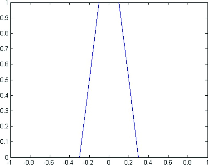
where the patch P_x denotes a neighborhood of x. u(x) and v(x) are the average intensities of the pixels in a patch inside and outside the contour, respectively. In order to specify the tubular region around the contour and analyze our model rigorously, for a fixed ε, we define a function B_ε(φ) as follows (Fig. 1):

$${\displaystyle B_{\epsilon }\left(\phi \right)=\left\{\begin{array}{cc}\hfill 1\hfill & \hfill \left|\phi \right|<\epsilon ,\hfill \\ \hfill \frac{1}{2}\left\{1+\frac{\phi +2\epsilon }{\epsilon }+\frac{1}{\pi }sin\left(\frac{\pi (\phi +2\epsilon )}{\epsilon }\right)\right\}\hfill & \hfill -3\epsilon <\phi \le -\epsilon ,\hfill \\ \hfill \frac{1}{2}\left\{1-\frac{\phi -2\epsilon }{\epsilon }+\frac{1}{\pi }sin\left(\frac{-\pi (\phi -2\epsilon )}{\epsilon }\right)\right\}\hfill & \hfill \epsilon \le \phi <3\epsilon ,\hfill \\ \hfill 0\hfill & \hfill \text{otherwise.}\hfill \end{array}\right.}$$ (7)

We denote by R_ε the region where B_ε(φ(x)) > 0, which is a banded region around the zero level set of φ. Since this banded region changes during the level set evolving, we call it an active band. Our local region energy functional is obtained by calculating E_x on all the points in R_ε. Then the energy functional is

$${\displaystyle E_{\text{local}}=\underset{\mathrm{\Omega }}{\int }{B}_{\epsilon }\left(\phi \left(x\right)\right)E_x\text{d}x=\underset{\mathrm{\Omega }}{\int }{B}_{\epsilon }\left(\phi \left(x\right)\right)(\underset{y\in P_x}{\int }{(I-u\left(x\right))}^2{H}_{\epsilon }\left(\phi \left(y\right)\right)\text{d}y+\underset{y\in P_x}{\int }{(I-v\left(x\right))}^2(1-H_{\epsilon }\left(\phi \left(y\right)\right))\text{d}y)\text{d}x.}$$ (8)

For a fixed level set function φ, u(x) and v(x) can be updated by

$${\displaystyle u\left(x\right)=\frac{\underset{y\in P_x}{\int }{H}_{\epsilon }\left(\phi \left(y\right)\right)I\left(y\right)\text{d}y}{\underset{y\in P_x}{\int }{H}_{\epsilon }\left(\phi \left(y\right)\right)\text{d}y},v\left(x\right)=\frac{\underset{y\in P_x}{\int }(1-H_{\epsilon }\left(\phi \left(y\right)\right))I\left(y\right)\text{d}y}{\underset{y\in P_x}{\int }(1-H_{\epsilon }\left(\phi \left(y\right)\right))\text{d}y}.}$$ (9)

FIG. 1.

An example of B_ε(φ), ε = 0.1.

3.B. Edge descriptor

Due to the poor quality of ultrasound images, some parts of a prostate boundary are often not clear. Also there are unwanted edges between the prostate and its surrounding areas. Most of the traditional methods fail in segmentation of the prostate from ultrasound images. In order to detect weak boundaries and avoid unwanted edges, we incorporate edge-based information into our energy functional.

The normal prostate gland has a homogenous, low-level uniform echo pattern. In ultrasound prostate images, the prostate regions are usually darker than their surrounding areas. Therefore, the intensity of pixels inside a prostate region is smaller than that of the pixels surrounding it. The intensity transition from inside to outside a prostate is from dark to bright. For each φ, at any point x on φ = 0, we introduce the following energy function:

$${\displaystyle \widetilde{E_x}=\underset{y\in {\tilde{P}}_x}{\int }H\left(\phi \left(y\right)\right)(\widetilde{v\left(x\right)}-\widetilde{u\left(x\right)})\text{d}y,}$$

which is taken as an edge descriptor. Here $\widetilde{P_x}$ is a patch along the normal direction of φ and centered at x. The size of $\widetilde{P_x}$ is (2m + 1) × 3, (m > 1). m is a positive integer chosen by users. $\widetilde{u\left(x\right)}$ and $\widetilde{v\left(x\right)}$ are the average intensities in ${\tilde{P}}_x\cap {\mathrm{\Omega }}_{\text{in}}$ and ${\tilde{P}}_x\cap {\mathrm{\Omega }}_{\text{out}}$, respectively. $\widetilde{E_x}$ describes the average intensities difference between ${\tilde{P}}_x\cap {\mathrm{\Omega }}_{\text{in}}$ and ${\tilde{P}}_x\cap {\mathrm{\Omega }}_{\text{out}}$. We summate $\widetilde{E_x}$ on all the points on φ = 0 to get an energy functional to describe boundary intensity difference, which has the following form:

$${\displaystyle \widetilde{E_{\text{edge}}}=-\underset{\phi =0}{\int }\widetilde{E_x}\text{d}x=-\underset{\phi =0}{\int }\underset{y\in {\tilde{P}}_x}{\int }H\left(\phi \left(y\right)\right)(\widetilde{v\left(x\right)}-\widetilde{u\left(x\right)})\text{d}y\text{d}x.}$$ (10)

Since we need to minimize the total energy functional, a minus sign is added.

In order to establish a variational framework, we extend the $\widetilde{E_{\text{edge}}}$ on φ = 0 to an energy on R_ε which is defined by

$${\displaystyle E_{\text{edge}}=-\underset{R_{\epsilon }}{\int }\widetilde{E_x}\text{d}x=-\underset{\mathrm{\Omega }}{\int }{B}_{\epsilon }\left(\phi \left(x\right)\right)\underset{y\in {\tilde{P}}_x}{\int }H\left(\phi \left(y\right)\right)(\widetilde{v\left(x\right)}-\widetilde{u\left(x\right)})\text{d}y\text{d}x.}$$ (11)

Note that $\underset{\epsilon \to 0}{lim}{E}_{\text{edge}}=\widetilde{E_{\text{edge}}}$. As φ is evolving to the true prostate boundary, E_edge approaches to its minimum. In other words, when the zero level set of φ is on the prostate boundary, E_edge achieves its minimum. We use Fig. 2 to illustrate $\widetilde{E_x}$ and $\widetilde{E_{\text{edge}}}$. In Fig. 2(a), we extract one column of the image intensity in ${\tilde{P}}_x$ and show it as a 1-D signal in Fig. 2(b). There is an obvious intensity gap at the prostate boundary. Thus ${\tilde{E}}_x$ achieves its maximum when x locates on the prostate boundary. Minimizing E_edge drives the level set approaching to the prostate boundary. Figure 2(c) shows a simplifying situation. The blue line is the true prostate boundary. The red and yellow lines are two different zero level sets. There are four patches with center points on these lines. x₂ and x₄ are on the prostate boundary. Suppose that x₁ and x₃ move to x₂ and x₄, respectively, during the contour evolution. It can be seen that $\widetilde{E_{x_1}}<\widetilde{E_{x_2}}$ and $\widetilde{E_{x_3}}<\widetilde{E_{x_4}}$. So the maximum of ${\tilde{E}}_x$ is achieved when x is on the boundary. Thus the minimum of E_edge is achieved when zero level set of φ coincides with the prostate boundary.

FIG. 2.

${\tilde{E}}_x$ and $\widetilde{E_{\text{edge}}}$. (a) An example of the edge descriptor. (b) The image intensity extracted from a patch along the normal direction of the prostate boundary as a 1-D signal. Note that only when x is located on the red point, the edge profile energy achieves its maximum. (c) A simplifying case. Patches are along the normal directions of the level sets. For fixed patch size, $\widetilde{max\left(E_x\right)}$ is achieved on the boundary.

3.C. Total variation level set formulation

With the above defined energy terms E_local and E_edge, we define the total energy functional in our model as

$${\displaystyle E={\alpha }_1{E}_{\text{local}}+{\alpha }_2{E}_{\text{edge}}+\gamma R\left(\phi \right)={\alpha }_1\underset{\mathrm{\Omega }}{\int }{B}_{\epsilon }\left(\phi \left(x\right)\right)(\underset{y\in P_x}{\int }{(I-u\left(x\right))}^2{H}_{\epsilon }\left(\phi \left(y\right)\right)\text{d}y+\underset{y\in P_x}{\int }{(I-v\left(x\right))}^2(1-H_{\epsilon }\left(\phi \left(y\right)\right))\text{d}y)\text{d}x-{\alpha }_2\underset{\mathrm{\Omega }}{\int }{B}_{\epsilon }\left(\phi \left(x\right)\right)\underset{y\in \widetilde{P_x}}{\int }H\left(\phi \left(y\right)\right)(\widetilde{v\left(x\right)}-\widetilde{u\left(x\right)})\text{d}y\text{d}x+\gamma \underset{\mathrm{\Omega }}{\int }{\delta }_{\epsilon }\left(\phi \right)\left|\nabla \phi \right|\text{d}x.}$$ (12)

By taking the first variation of the energy functional with respect to φ, we can get the updating equation of φ (see the Appendix),

$${\displaystyle \frac{\partial \phi }{\partial t}=B_{\epsilon }\left(\phi \left(x\right)\right)(-{\alpha }_1\underset{y\in P_x}{\int }{\delta }_{\epsilon }\left(\phi \left(y\right)\right){(I\left(y\right)-u\left(x\right))}^2-{(I\left(y\right)-v\left(x\right))}^2\text{d}y+{\alpha }_2\underset{y\in \widetilde{P_x}}{\int }{\delta }_{\epsilon }\left(\phi \left(y\right)\right)(\widetilde{v\left(x\right)}-\widetilde{u\left(x\right)})\text{d}y)+\gamma {\delta }_{\epsilon }\phi \left(x\right)\text{div}\left(\frac{\nabla \phi \left(x\right)}{\left|\nabla \phi \left(x\right)\right|}\right).}$$ (13)

Here $B_{\epsilon }^{\prime }\left(\phi \left(x\right)\right)$ denotes the derivative of B_ε(φ(x)). $B_{\epsilon }^{\prime }\left(\phi \left(x\right)\right)$ is equal to zero in the banded area, so it does not affect the evolution of the contour.

It is worth noting that without the second term, Eq. (13) has the same form with updating equation of φ in Ref. 33. In this case, our model can be seen as a smooth version of Eq. (6) in Ref. 33. By introducing the function B_ε(φ(x)), our method only focuses on the pixels in the tubular region: $\{x\in \mathrm{\Omega },|\left|\phi \left(x\right)\right|\le \epsilon \}$.

4. EXPERIMENT RESULTS

In order to illustrate the effectiveness of our proposed method, that is, the proposed method can segment ultrasound images of prostates with weak boundaries and unwanted edges, we carry out experiments on two kinds of images: 2D single images and 3D volume images. We choose 100 typical 2D ultrasound images with intensity inhomogeneities, weak boundaries, and unwanted edges to evaluate the performance of our method. The proposed segmentation method has also been tested on 13 3D TRUS sequences from 13 different patients from Brigham Women’s Hospital. Each 3D volume consists of 10–14 2D images, totally 136 2D images. The size of each 2D image is 512 × 512 with a pixel size of 0.3125 × 0.3125 mm. All the experiments are implemented with matlab R2011a on the PC of CPU 2.5 GHz, RAM 6.00G.

4.A. Single image segmentation

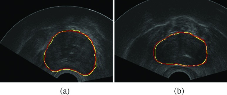
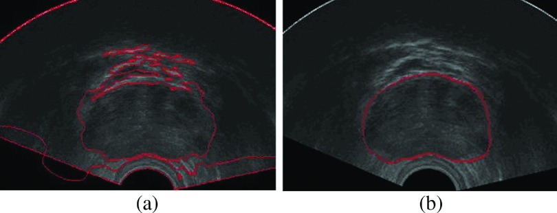
Figure 3 shows the evaluation of our segmentation results on 2D prostate ultrasound images. As we can see in Fig. 4, segmentation results of RSF model³² and our model on the same prostate ultrasound images are displayed. The RSF model has a good performance on inhomogeneous images like MRI. But for ultrasound images, the RSF model cannot produce acceptable segmentation results due to the characteristic artifacts of ultrasound images: attenuation, speckles, shadows, signal dropout, visually invisible boundaries, etc. Although the RSF model considers the local area at each pixel x, the evolution of the level sets still uses the information of all the image pixels. For the prostate ultrasound images in our experiments, the imaging areas are fan-shaped regions. Outside these regions, the values of pixels are equal to zero. If we directly compute the region scalable fitting energy, the pixels outside a fan-shaped region are also calculated as mean intensity outside the contour. These pixels greatly affect the final segmentation results. In our experiments, the RSF model produces oversegmentation results. In contrast, in our algorithm, only the pixels in R_ε have contribution to the evolution of the contour. When the contour is evolving toward the true boundary of the prostate, the average intensities inside and outside the contour will converge to the local mean intensities inside and outside the prostate, respectively.

FIG. 3.

Segmentation result on 2D images. The red contours are done manually by ultrasound experts and the yellow ones are our segmentation results. (See color online version.)

FIG. 4.

(a) The segmentation result of the RSF model. (b) The segmentation result of our algorithm.

In order to evaluate the performance of our algorithm, we select 100 typical 2D ultrasound prostate images from our data set and test our algorithm on them. The 100 typical 2D ultrasound images are usually corrupted with intensity inhomogeneities, weak boundaries, and unwanted edges. For each image, the size is 512 × 512. The mean segmentation time of 100 ultrasound images of our method is about 30 s. We compute the DSC and sensitivity (Se) of the 100 prostate ultrasound images. The validation results show that our method can obtain a sensitivity of 94.87% ± 1.85% and a DSC of 95.82% ± 2.23%. The sensitivity and DSC are computed as follows:

DSC:

$${\displaystyle \text{DSC}=2(V_m\cap V_a)/(V_m+V_a),}$$

sensitivity:

$${\displaystyle \text{Se}=V_m\cap V_a/V_m.}$$

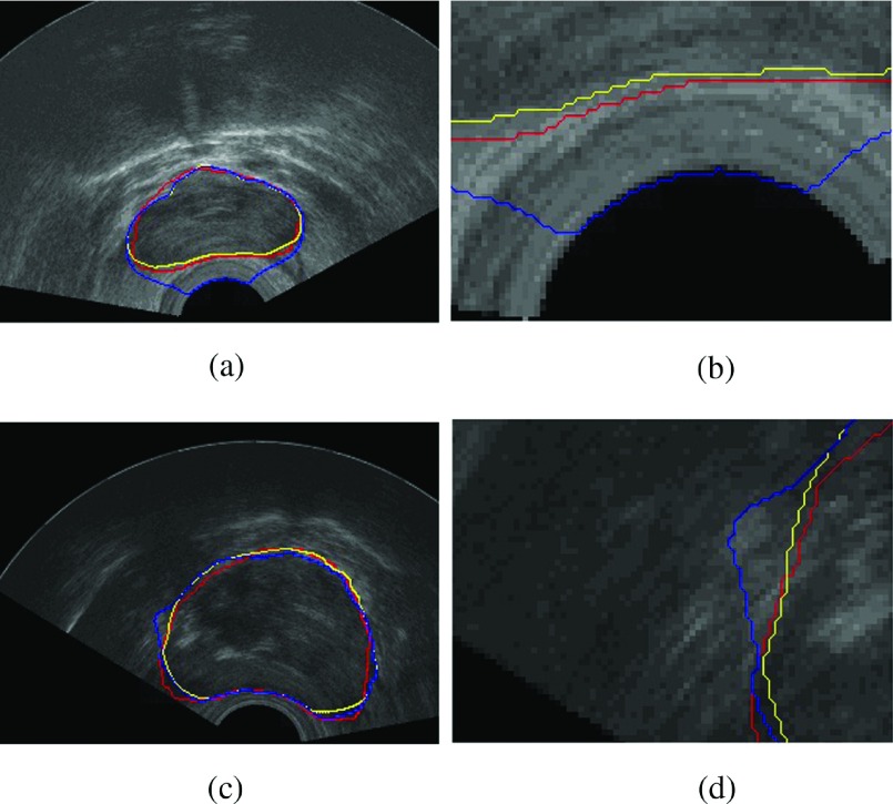
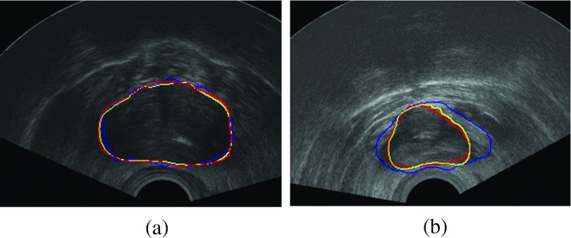
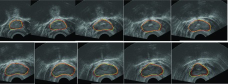
As an example, in Fig. 5, we select 12 images from the 100 typical images and show their segmentation results. Red contours are manually delineated and yellow contours are our segmentation results. We also compare segmentation results on the same image with and without E_edge described in Sec. 3.C. In Fig. 6, the first column shows segmentation results on two different images. The red contours are delineated by a radiologist. The blue contours are segmentation results without the edge descriptor. The yellow contours are segmentation results with the edge descriptor. The second column shows the details in zoom. Due to the insertion of the ultrasound probe, there are strong edges between fan-shaped imaging areas and the probe. Top right shows how the probe affects the final segmentation results. If the initial contour is close to the probe, the final contour may stuck into the strong edges. By properly setting the size of the edge descriptor, we can avoid this situation.

FIG. 5.

Segmentation results of 12 ultrasound prostate images. Manual segmentation results are shown in red, and our segmentation results are shown in yellow. (See color online version.)

FIG. 6.

Column 1: the segmentation results of two ultrasound images. Column 2: zooming in on details. The red contours are drawn by radiologist, the blue contours are the segmentation result without the edge descriptor, and the yellow contours are the segmentation result with the edge descriptor. (See color online version.)

4.B. Volume segmentation

For volume image segmentation, the proposed method can be divided into four steps: (1) the midgland, apex, and base slices are first selected. On the midgland slice, we select five to eight initial points to generate the initial contour. (2) The proposed segmentation method is used to get fine segmentation of the midgland slice by deforming the initial contours. (3) The segmented results of midgland slices are then propagated to their adjacent slices and used as their initial contours. We adopt step (2) to segment these slices. This procedure is repeated until all the 2D slices of the 3D volume image are segmented but the apex, base slices. (4) For any apex or base slice to be segmented, we use normalized cross-correlation based template matching method to estimate the position of the prostate in the slice. Then we use mean-shapes calculated from our data set as initial contours. Step (2) is also used to segment these slices.

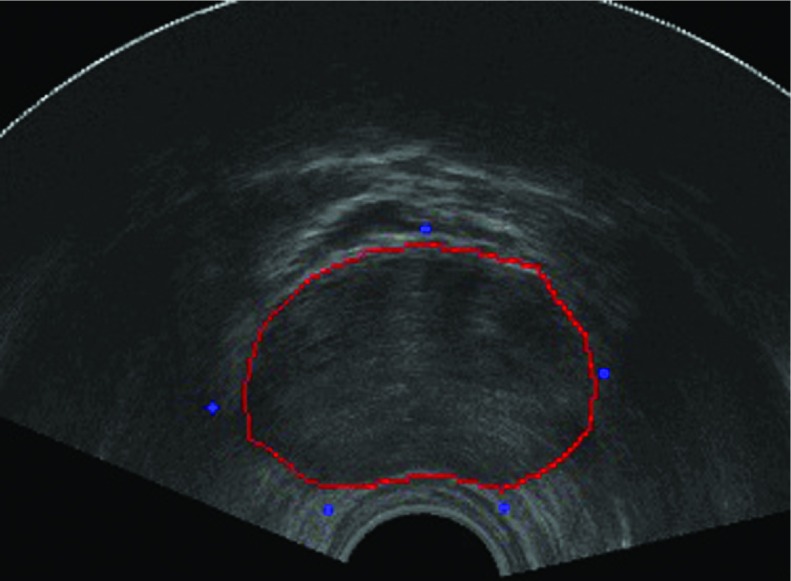
A 3D ultrasound prostate volume consists of a set of 2D prostate image slices. Selection of midgland, apex, and base slices is the first step in our algorithm. In our experiments, we just take the middle slice as midgland slice and the first and last slices as apex and base, respectively, in each volume image. We initialize the proposed algorithm by manually selecting five to eight points in the midgland slice. The initial points are located in the following regions of the prostate: anterior, posterior, right, left, right-posterior, and left-posterior. The initial points are not required to be located exactly on the prostate boundary. Actually in our experiments, it is enough to mark initial points in the near region of the prostate boundary. Figure 7 shows one example of the initial points.

FIG. 7.

The blue dots are the selected initial points. (See color online version.)

4.B.1. Initialization and segmentation of apex and base of the prostate

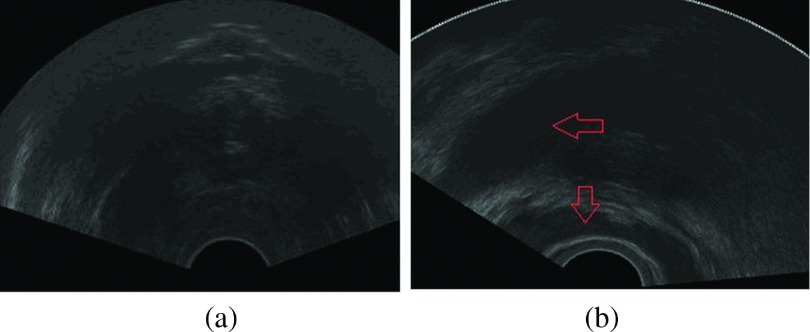
As we can see in Fig. 8, the prostate is usually invisible in the apex slices. In the base slices, the prostate boundaries are often corrupted by other organs like seminal vesicle and bladder. After finishing step (3), if we directly use the segmentation results of their adjacent slices as initialization on apex and base slices, it is very difficult to get correct prostate boundaries. To solve this, we utilize normalized cross-correlation based template matching to detect the region of interest (ROI) in apex and base slices. After we get the prostate ROI, the initialization strategy is to calculate the mean shapes of apex and base of the prostate from our data set, then to align the derived mean shapes to the ROIs.

FIG. 8.

Ultrasound image of the prostate apex and base slice. (a) The boundary of the prostate is visually invisible. (b) The prostate base is influenced by the seminal vesicle and bladder. Regions with red arrows are the bladder and seminal vesicle. (See color online version.)

Since we have the prostate contours from adjacent slices, we can use these contours to construct templates which contain the whole prostate region. Our goal is to find the best matching patches in the apex and base slices. The best matching patches are the patches having the best displacement defined in Eq. (14).

The normalized cross-correlation has been commonly used as a metric to evaluate the similarity (dissimilarity) between two images. The normalized cross-correlation between the image I and a template T in the discrete image domain with a displacement d = (d_i, d_j) can be defined as the point product of two vectors,

$${\displaystyle (I,T)\left(d\right)=\sum _{i,j}〈\delta I(i,j),\delta T(i+d_i,j+d_j)〉,}$$

where δI(i, j) is defined as $I(i,j)-\overline{I}(i,j)/\Vert I(i,j)-\overline{I}(i,j)\Vert$, ‖ ⋅ ‖ is the L₂ norm, and δT(i, j) has the same form with δI(i, j).

For a given image and a template, the best displacement which corresponds to the maximum of the normal cross-correlation function is

$${\displaystyle d_{\text{best}}=arg\underset{d}{max}(I,T)\left(d\right),}$$ (14)

where d_best is the best displacement that the template will move.

Because apex and base of a prostate are not always visible, we use manual segmentation results of apex slices and base slices in this stage. While segmenting one image, we randomly choose six contours of apex and base slices in our data set to calculate the mean shapes of apex and base. Compared with statistical shape methods, this is a preprocessing stage. We only need one mean shape as an initial contour. The mean shape is computed as follows:

1. Align all the binary shapes. We just take the first image as reference and simply align other images to the first one.

2. Computing the mean shape. If {S₁, …, S_N} is a set of manual segmentation results of apex slices, the mean shape of apex slice of the ith image is

$${\displaystyle M_i=\frac{1}{N}\sum _{j\ne i}^N{S}_j,i=1,\dots ,N,}$$ (15)

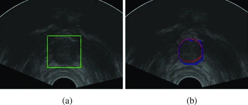
where S_i, i = 1, …, N denote the manual segmentation results of the apex slices. Mean shapes of the base slices can be obtained in the same way. After we get the prostate ROI, we can use the average shape to initialize the segmentation method in step (2). This step is indicated in Fig. 9.

FIG. 9.

(a) The prostate ROI detected by normalized cross-correlation between previous slice and current slice. (b) The segmentation result of mean-shape initialization on a new apex slice. The red contour is the manual segmentation result and the blue contour is our segmentation result. (See color online version.)

4.B.2. Experiments on volume images

Figure 10 compares the segmentation results of our method and the method described in Ref. 6 on the midgland slices. In Ref. 6, the authors used the gradient vector field (GVF) of the prostate ultrasound images as external force of a parametric active contour model. We test their method and the proposed algorithm on the same slices with the same initializations. The first row shows a better segmentation result near the midgland of a prostate. Both algorithms can get the prostate boundary. But our algorithm performance is better than that of the method in Ref. 6 compared with the manual segmentation results. For a slice near the base, the method in Ref. 6 fails to capture the prostate boundary when the nonprostate area appears similar texture information with the prostate area.

FIG. 10.

Segmentation results compared with the manual delineations. The red contours are drawn by radiologist, the blue contours are the segmentation results using algorithm mentioned in Ref. 6, and the yellow contours are our segmentation results. (See color online version.)

Segmentation results of the proposed method on one 3D volume sequence are shown slice by slice in Fig. 11. Table I indicates the values of parameters in our algorithm. The length of the edge descriptor m is defined by a user. We can choose large m to deal with fake boundaries. Smaller m is more efficient for weak boundaries. During our experiments, we have found that m = 6 can get good segmentation results for most of our images. For quantitatively evaluating the performance of the proposed segmentation method, the following metrics are used.

FIG. 11.

Segmentation results of one TRUS volume sequence, from apex to base. Manual segmentation results are shown in red, and our segmentation results are shown in yellow. (See color online version.)

TABLE I.

Coefficients in the proposed algorithm.

	Coefficients				Patch size	Edge descriptor
	α1	α2	ε	γ	P	M
Values	0.5	0.5	1.5	1.2	6	User defined

Error: the absolute magnitude of the nonoverlapping regions between two delineated prostates is defined as

$${\displaystyle \text{Err}=\frac{|A_a+A_b-A_{a\cap b}|}{A_a+A_b}\times 100\%.}$$

Difference: the difference between two delineated prostates is defined as

$${\displaystyle \text{Diff}=\frac{A_a-A_b}{A_b}\times 100\%.}$$

Hausdorff distance:

$${\displaystyle \text{HD}=max(supinfd(C_a,C_b),supinfd(C_b,C_a)).}$$

Volume difference:

$${\displaystyle \text{VD}=|V_a-V_b|.}$$

Here A_a, A_b, V_a, V_b are the areas and volumes of two contours a and b. d(C_a, C_b) is the distance between two contours a and b. We compare our algorithm with the method in Refs. ⁶ and ⁷ using the metrics above. Tables II and III show accuracy comparison in apex and base slices. Both Refs. ⁶ and ⁷ are based on the edge information. Reference ⁷ needs initial points very close to the prostate boundaries. In our experiments, the initial points are not strict. Thus, their methods could not get promising segmentation results, especially in the apex and base slices using our initialization. Table IV compares accuracy of segmentation of our algorithm and algorithms in Refs. ⁶ and ⁷ in midgland slices.

TABLE II.

Comparison of segmentation results in apex of our algorithm and algorithm in Refs. ⁶ and ⁷ in three metrics.

		P1	P2	P3	P4	P5	P6	P7	P8	P9	P10	P11	P12	P13
Err	Our	6.78	5.53	6.47	9.89	6.44	7.61	10.02	6.84	13.50	9.06	11.21	9.84	11.27
	Reference 6	18.25	10.00	19.90	12.57	19.08	18.29	18.21	20.50	23.43	18.50	19.33	17.86	20.03
	Reference 7	20.05	13.03	20.96	13.80	20.04	22.00	24.99	23.72	25.68	20.45	22.30	19.28	24.23
Diff	Our	11.31	1.02	5.58	8.4	7.02	6.89	3.27	6.17	9.15	5.83	16.16	4.28	10.20
	Reference 6	27.23	17.80	24.72	14.55	43.02	44.53	37.37	26.82	27.37	18.46	39.89	20.01	24.42
	Reference 7	30.47	19.64	22.14	16.28	50.04	56.40	44.65	30.71	38.14	20.18	49.20	24.75	29.58
HD	Our	2.44	1.98	2.19	2.80	2.14	2.10	2.22	1.82	4.00	1.87	2.83	2.37	2.80
	Reference 6	5.63	4.94	4.61	4.34	4.20	4.38	4.07	5.22	4.01	4.79	5.23	5.03	4.70
	Reference 7	7.64	5.03	6.33	5.09	6.73	7.34	6.04	7.35	7.48	7.26	7.90	8.02	7.00

TABLE III.

Comparison of segmentation results in base of our algorithm and algorithm in Refs. ⁶ and ⁷ in three metrics.

		P1	P2	P3	P4	P5	P6	P7	P8	P9	P10	P11	P12	P13
Err	Our	6.40	8.31	5.00	7.66	9.26	5.44	4.6	10.97	6.53	3.97	9.51	7.68	11.43
	Reference 6	14.34	12.96	11.86	13.53	19.27	9.67	12.61	13.45	9.44	14.15	15.26	14.49.	13.00
	Reference 7	16.54	17.02	15.09	19.15	19.98	13.11	14.14	15.23	15.86	16.35	18.20	19.44	20.77
Diff	Our	7.05	10.60	5.88	12.06	14.28	4.91	3.02	4.60	5.35	6.81	6.50	12.20	9.82
	Reference 6	21.95	25.74	25.02	27.37	47.32	16.29	21.18	22.35	27.46	17.28	22.64	22.00	25.22
	Reference 7	27.74	26.01	26.34	28.80	48.23	26.71	29.49	26.75	28.14	26.71	29.22	22.79	26.80
HD	Our	2.33	3.53	3.11	2.37	2.83	2.56	2.31	4.05	2.70	1.98	2.19	2.67	3.33
	Reference 6	4.85	6.73	6.20	6.13	8.20	4.91	6.25	5.03	4.91	5.82	5.74	6.88	6.90
	Reference 7	5.93	8.33	6.94	6.59	8.64	5.26	6.37	6.55	7.37	8.20	7.95	8.62	9.00

TABLE IV.

Comparison of segmentation results in midgland of our algorithm and algorithm in Refs. ⁶ and ⁷ in three metrics.

		P1	P2	P3	P4	P5	P6	P7	P8	P9	P10	P11	P12	P13
Err	Our	4.71	3.26	3.33	2.36	2.51	2.15	2.31	3.21	2.36	3.97	5.46	4.76	8.83
	Reference 6	10.46	9.70	11.86	6.26	10.5	8.43	6.20	10.24	8.55	9.82	10.06	10.27	12.00
	Reference 7	12.17	10.71	6.61	8.47	11.9	9.64	9.68	11.35	9.89	11.20	12.23	12.79	14.85
Diff	Our	0.47	1.61	2.31	1.07	2.10	0.43	0.79	1.20	1.26	1.38	2.26	2.57	4.10
	Reference 6	17.56	20.02	9.00	9.02	20.17	14.91	12.56	10.06	9.90	11.42	18.83	19.81	22.26
	Reference 7	20.92	21.24	13.58	14.23	22.01	16.34	16.65	15.75	13.99	14.82	20.69	20.11	24.58
HD	Our	2.57	2.18	1.56	1.25	0.99	1.88	1.13	1.82	1.25	1.33	2.67	1.77	2.67
	Reference 6	5.30	4.69	4.58	4.34	3.22	3.91	3.38	4.04	4.88	3.29	5.90	3.86	6.02
	Reference 7	5.32	5.20	3.80	5.09	4.86	4.06	3.95	5.51	5.85	5.00	6.11	4.95	7.91

Also we compute DSC and sensitive (Se) on the whole data set. The validation results show that our method can obtain a sensitivity of 93.16% ± 2.30, a DSC of 94.03 ± 1.5%, and a Vd of 2.61 ± 0.63 cm³.

It is difficult to compare our results to other results from segmentation algorithms using 3D TRUS images due to the differences of data sets used and evaluation metrics. However, the DSC and sensitivity (Se) of our algorithm are compared with the best segmentation accuracy reported in Refs. ^{16, 17}, and ²⁰ (Table V). The mean sensitivity of 93.16% ± 2.30% obtained by our algorithm is better than 87.7% ± 4.9% obtained in Ref. 17. The mean DSC of 94.03% ± 1.5% of our method is comparable to a sensitivity of 93.2% ± 2.0% obtained in Ref. 16. The mean volume difference of 2.61 ± 0.63 cm³ is comparable to a volume difference of 2.6 ± 1.9 cm³ obtained by Ref. 17. Our method shows advantage of accuracy in some sense.

TABLE V.

Comparison with other 3D TRUS segmentation methods.

	Reference 16	Reference 17	Reference 20	Our
DSC (%)	93.2 ± 2.0	93.1 ± 1.6	90.3 ± 2.3	94.03 ± 1.50
SE (%)	—	93.0 ± 2.0	87.7 ± 4.9	93.16 ± 2.30
VD (cm3)	2.4 ± 1.6	2.6 ± 1.9	—	2.61 ± 0.63

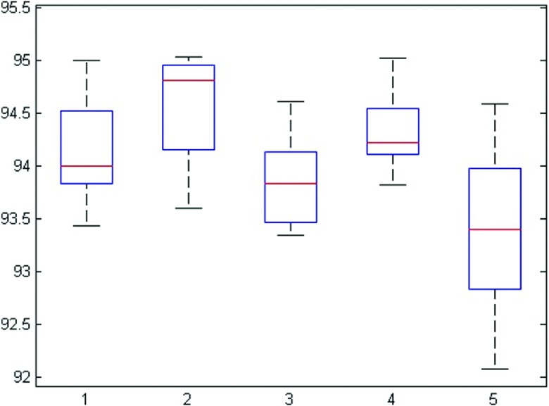
Five images are randomly selected for evaluating the reproducibility and initialization robustness of the proposed algorithm. Each image is segmented five times with different initializations. Figure 12 shows the DSC for five repeated segmentations. This experiment shows that the DSC values are consistent and show very small variations across different initializations.

FIG. 12.

DSC of each image with different initializations.

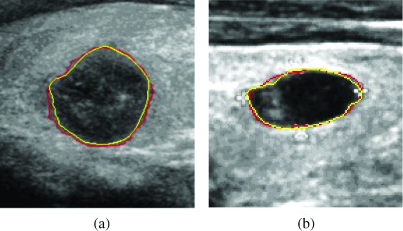
Our segmentation model can also segment tissues having similar sonographic appearance with the prostate (e.g., cysts and thyroid nodules). We apply our model to segment the ultrasound thyroid nodule images. Figure 13 shows the segmentation results.

FIG. 13.

Segmentation results of the ultrasound thyroid nodule images. Yellow contours are delineated by a radiologist. Red contours are segmentation results of our model.

5. CONCLUSION

In this paper, a novel efficient segmentation method for ultrasound images of prostates with weak boundaries is proposed. As we know, most of the existing methods cannot get promising prostate contours when segmenting ultrasound images with weak boundaries and unwanted edges. The energy functional of the proposed model is mainly composed of a local region based energy and an edge-based energy. Our method can capture local image information in an active band around the zero level set. The local region based energy is determined by local image intensity in an active band. Furthermore, we incorporate edge-based information to exploit the intensity variation in patches along the normal directions of the evolving contour, which is helpful in detecting of weak boundary and avoiding unwanted edges in the ultrasound images. Also an initialization strategy based on the mean shapes and the normalized cross-correlation for apex and base slices is given. In order to illustrate that the proposed method can segment ultrasound images of prostates with weak boundaries and unwanted edges, we have carried out experiments on both 3D volume images and 2D images. Comparisons with other approaches have been performed to show the effectiveness and advantages of the proposed method. Our method has the potential to be extended to other applications where the objects to be segmented have similar sonographic appearance with the prostate. Since we do not use any acceleration or any fast algorithm in our method, the mean segmentation time of the proposed method is unsatisfactory in some sense. We would like to explore the possibilities of accelerating our algorithm with GPU based programming to assist in TRUS guided biopsies in the future.

APPENDIX: DERIVATION OF THE GRADIENT FLOW

The total energy functional in our model is

$${\displaystyle E={\alpha }_1{E}_{\text{local}}+{\alpha }_2{E}_{\text{edge}}+\gamma R\left(\phi \right)={\alpha }_1\underset{\mathrm{\Omega }}{\int }{B}_{\epsilon }\left(\phi \left(x\right)\right)(\underset{y\in P_x}{\int }{(I-u\left(x\right))}^2{H}_{\epsilon }\left(\phi \left(y\right)\right)\text{d}y+{\lambda }_2\underset{y\in P_x}{\int }{(I-v\left(x\right))}^2(1-H_{\epsilon }\left(\phi \left(x\right)\right))\text{d}y)\text{d}x-{\alpha }_2\underset{\mathrm{\Omega }}{\int }{B}_{\epsilon }\left(\phi \left(x\right)\right)\underset{y\in \widetilde{P_x}}{\int }H\left(\phi \left(y\right)\right)(\widetilde{v\left(x\right)}-\widetilde{u\left(x\right)})\text{d}y\text{d}x+\gamma \underset{\mathrm{\Omega }}{\int }{\delta }_{\epsilon }\left(\phi \right)\left|\nabla \phi \right|\text{d}x.}$$ (A1)

By taking the first variation of the energy functional with respect to φ, we can get the updating equation of φ,

$${\displaystyle \frac{\partial \phi }{\partial t}=-\{{\alpha }_1{B}_{\epsilon }\left(\phi \left(x\right)\right)(\underset{y\in P_x}{\int }{\delta }_{\epsilon }\left(\phi \left(y\right)\right){(I\left(y\right)-u\left(x\right))}^2-{(I\left(y\right)-v\left(x\right))}^2\text{d}y+{\alpha }_1{B}_{\epsilon }^{\prime }\left(\phi \left(x\right)\right)(\underset{y\in P_x}{\int }{H}_{\epsilon }\left(\phi \left(y\right)\right){(I\left(y\right)-u\left(x\right))}^2\text{d}y+\underset{y\in P_x}{\int }(1-H_{\epsilon }\left(\phi \left(y\right)\right)){(I\left(y\right)-v\left(x\right))}^2\text{d}y-{\alpha }_2{B}_{\epsilon }\left(\phi \left(x\right)\right)\left(\underset{y\in \widetilde{P_x}}{\int }{\delta }_{\epsilon }\left(\phi \left(y\right)\right)(\widetilde{v\left(x\right)}-\widetilde{u\left(x\right)})\text{d}y\right)+{\alpha }_2{B}_{\epsilon }^{\prime }\left(\phi \left(x\right)\right)\left(\underset{y\in \widetilde{P_x}}{\int }{H}_{\epsilon }\left(\phi \left(y\right)\right)(\widetilde{v\left(x\right)}-\widetilde{u\left(x\right)})\text{d}y\right))\}+\gamma {\delta }_{\epsilon }\phi \left(x\right)\text{div}\left(\frac{\nabla \phi \left(x\right)}{\left|\nabla \phi \left(x\right)\right|}\right),}$$ (A2)

where $B_{\epsilon }^{\prime }\left(\phi \left(x\right)\right)$ denotes the derivative of B_ε(φ(x)). $B_{\epsilon }^{\prime }\left(\phi \left(x\right)\right)$ is equal to zero in the banded area, so it does not affect the evolution of the contour. Then the updating equation of φ becomes

$${\displaystyle \frac{\partial \phi }{\partial t}=B_{\epsilon }\left(\phi \left(x\right)\right)(-{\alpha }_1\underset{y\in P_x}{\int }{\delta }_{\epsilon }\left(\phi \left(y\right)\right){(I\left(y\right)-u\left(x\right))}^2-{(I\left(y\right)-v\left(x\right))}^2\text{d}y+{\alpha }_2\underset{y\in \widetilde{P_x}}{\int }{\delta }_{\epsilon }\left(\phi \left(y\right)\right)(\widetilde{v\left(x\right)}-\widetilde{u\left(x\right)})\text{d}y)+\gamma {\delta }_{\epsilon }\phi \left(x\right)\text{div}\left(\frac{\nabla \phi \left(x\right)}{\left|\nabla \phi \left(x\right)\right|}\right).}$$

The partial differential equation (13) can be implemented with finite difference scheme. All the spatial partial derivatives ∂φ/∂x and ∂φ/∂y in our model are approximated by the central difference. The temporal partial derivative ∂φ/∂t is approximated by the forward difference. The level set evolution equation can be discretized by the following difference equation:

$${\displaystyle \frac{{\phi }_{i,j}^{n+1}-{\phi }_{i,j}^n}{\mathrm{\Delta }t}=F\left({\phi }_{i,j}^n\right)+R\left({\phi }_{i,j}^n\right),}$$ (A3)

where $F\left({\phi }_{i,j}^n\right)$ and $R\left({\phi }_{i,j}^n\right)$ are the numerical approximation of the first two terms and last term of the right hand side in Eq. (13). Δt is the time step. By the Courant–Friedrichs–Lewy (CFL) condition,³⁴ Δt is given by Δt = 0.5/[max(F + R) + ε]. The space step h = 1 for the digital images. The second-order central differences are defined as follows:

$${\displaystyle {\phi }_x=\frac{{\phi }_{i+1,j}^n-{\phi }_{i-1,j}^n}{2h},{\phi }_y=\frac{{\phi }_{i,j+1}^n-{\phi }_{i,j-1}^n}{2h},{\phi }_{xx}=\frac{{\phi }_{i+1,j}^n+{\phi }_{i-1,j}^n-2{\phi }_{i,j}^n}{h^2},{\phi }_{yy}=\frac{{\phi }_{i,j+1}^n+{\phi }_{i,j-1}^n-2{\phi }_{i,j}^n}{h^2},{\phi }_{xy}=\frac{{\phi }_{i+1,j+1}^n+{\phi }_{i-1,j-1}^n-{\phi }_{i-1,j+1}^n-{\phi }_{i+1,j-1}^n}{h^2}.}$$ (A4)

The corresponding curvature div(∇φ(x)/|∇φ(x)|) in the regularization term $R\left({\phi }_{i,j}^n\right)$ is calculated by

$${\displaystyle \kappa =\text{div}\left(\frac{\nabla \phi \left(x\right)}{\left|\nabla \phi \left(x\right)\right|}\right)=\frac{{\phi }_{xx}{\phi }_y^2-2{\phi }_{x,y}{\phi }_x{\phi }_y+{\phi }_{yy}{\phi }_x^2}{{({\phi }_x^2+{\phi }_y^2)}^{\frac{3}{2}}}.}$$ (A5)

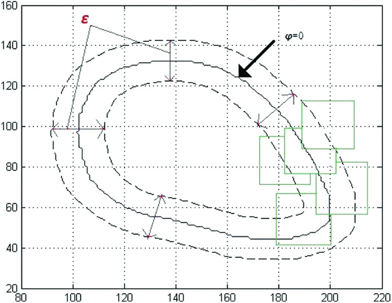
We adopt the narrow band method proposed by Adalsteinsson and Sethian³⁵ to solve Eq. (A1). B_ε(φ(x)) defines a banded region,

$${\displaystyle R_{\epsilon }=\{x\in \mathrm{\Omega },d(x,C)\le \epsilon \},}$$

where d is the distance between point x and contour C. Figure 14 shows the banded region and patches in it.

FIG. 14.

Banded region defined by B_ε(φ(x)) and patches in it.

After getting the banded region around the contour C, patches P and ${\tilde{P}}_x$ can be extracted. The local interior and exterior mean intensity values u and v in each patch P and the interior and exterior mean intensity values $\tilde{u}$ and $\tilde{v}$ in ${\tilde{P}}_x$ can be calculated. Then $F\left({\phi }_{i,j}^n\right)$ is

$${\displaystyle F\left({\phi }_{i,j}^n\right)={\alpha }_2\underset{y\in {\tilde{P}}_x}{\int }{\delta }_{\epsilon }{\phi }_{i,j}^n\left(y\right)({\tilde{v}}^{\left({\phi }_{i,j}^n\right)}-{\tilde{u}}^{\left({\phi }_{i,j}^n\right)})\text{d}y+B_{\epsilon }{\phi }_{i,j}^n\left(x\right)(-{\alpha }_1\underset{y\in P_x}{\int }{{\delta }_{\epsilon }{\phi }_{i,j}^n\left(y\right)(I\left(y\right)-u\left({\phi }_{i,j}^n\right))}^2-{(I\left(y\right)-v\left({\phi }_{i,j}^n\right))}^2\text{d}y).}$$ (A6)

We normalize F_n = F/max(F) during implementation. To prevent the level set function from becoming over flat, we use the reinitialization technique suggested by Sussman et al.³⁶

CONFLICT OF INTEREST DISCLOSURE

The authors have no COI to report.

REFERENCES

- 1.Jemal A., Freddie B., Melissa M. C., Jacques F., Elizabeth W., and Forman D., “Global cancer statistics,” Ca-Cancer J. Clin. 61(2), 69–90 (2011). 10.3322/caac.20107 [DOI] [PubMed] [Google Scholar]
- 2.Ferlay J., Shin H., Bray F., Forman D., Mathers C., and Parkin D., “Estimates of worldwide burden of cancer in 2008: Globocan 2008,” Int. J. Cancer 127(12), 2893–2917 (2010). 10.1002/ijc.25516 [DOI] [PubMed] [Google Scholar]
- 3.Nouranian S., Mahdavi S., Spadinger I., Morris W., Salcudean S., and Abolmaesumi P., “A multi-atlas-based segmentation framework for prostate brachytherapy,” IEEE Trans. Med. Imaging 4(34), 950–961 (2015). 10.1109/TMI.2014.2371823 [DOI] [PubMed] [Google Scholar]
- 4.Ladak H., Mao F., Wang Y., Downey D., Steinman D., and Fenster A., “Prostate boundary segmentation from 2D ultrasound images,” Med. Phys. 27(8), 1777–1788 (2000). 10.1118/1.1286722 [DOI] [PubMed] [Google Scholar]
- 5.Lobregt S. and Viergever M., “A discrete dynamic contour model,” IEEE Trans. Med. Imaging 14(1), 12–24 (1995). 10.1109/42.370398 [DOI] [PubMed] [Google Scholar]
- 6.Jendoubi A., Zeng J., and Chouikha M., “Segmentation of prostate ultrasound images using an improved snakes model,” in Proceedings of the International Conference on Signal Processing (IEEE, Beijing, China, 2004), Vol. 3, pp. 2568–2571. [Google Scholar]
- 7.Chiu B., Freeman G., Salama M., and Fenster A., “Prostate segmentation algorithm using dyadic wavelet transform and discrete dynamic contour,” Phys. Med. Biol. 49(21), 4943–4960 (2004). 10.1088/0031-9155/49/21/007 [DOI] [PubMed] [Google Scholar]
- 8.Yan P., Xu S., Turkbey B., and Kruecker J., “Adaptively learning local shape statistics for prostate segmentation in ultrasound,” IEEE Trans. Biomed. Eng. 58(3), 633–641 (2011). 10.1109/tbme.2010.2094195 [DOI] [PMC free article] [PubMed] [Google Scholar]
- 9.Yan P., Xu S., and Turkbey B., “Discrete deformable model guided by partial active shape model for TRUS image segmentation,” IEEE Trans. Biomed. Eng. 57(5), 1158–1166 (2010). 10.1109/tbme.2009.2037491 [DOI] [PMC free article] [PubMed] [Google Scholar]
- 10.Ghose S., Arnau O., Mart R., Llad X., Freixenet J., Mitra J., Vilanova J., Comet-Batlle J., and Meriaudeau F., “Statistical shape and texture model of quadrature phase information for prostate segmentation,” Int. J. Comput. Assisted Radiol. Surg. 7(1), 43–55 (2012). 10.1007/s11548-011-0616-y [DOI] [PubMed] [Google Scholar]
- 11.Kim S. and Seo Y., “A TRUS prostate segmentation using Gabor texture features and snake-like contour,” J. Inf. Process. Syst. 9(1), 103–116 (2013). 10.3745/JIPS.2013.9.1.103 [DOI] [Google Scholar]
- 12.Saroul L., Bernard O., Vray D., and Friboulet D., “Prostate segmentation in echographic images: A variational approach using deformable super-ellipse and Rayleigh distribution,” in 5th IEEE International Symposium on Biomedical Imaging: From Nano to Macro (IEEE, Paris, France, 2008), pp. 129–132. [Google Scholar]
- 13.Ding M. et al. , “Fast prostate segmentation in 3D TRUS images based on continuity constraint using an autoregressive model,” Med. Phys. 34(11), 4109–4125 (2007). 10.1118/1.2777005 [DOI] [PubMed] [Google Scholar]
- 14.Fan S., Ling K., and Sing N., “3D prostate surface detection from ultrasound images based on level set method,” in Medical Image Computing Computer-Assisted Intervention MICCAI, edited by Dohi T. and Kikinis R. (Springer, Berlin, Heidelberg, 2002), pp. 389–396. [Google Scholar]
- 15.Yu Y., Cheng J., Li J., Chen W., and Chiu B., “Automatic prostate segmentation from transrectal ultrasound images,” in IEEE Biomedical Circuits and Systems Conference (BioCAS) (IEEE, Lausanne, Switzerland, 2014), pp. 117–120. [Google Scholar]
- 16.Qiu W., Yuan J., Ukwatta E., Sun Y., Rajchl M., and Fenster A., “Prostate Segmentation: An efficient convex optimization approach with axial symmetry using 3-D TRUS and MR images,” IEEE Trans. Med. Imaging 33(4), 947–959 (2014). 10.1109/tmi.2014.2300694 [DOI] [PubMed] [Google Scholar]
- 17.Qiu W., Yuan J., Ukwatta E., Tessier D., and Fenster A., “3-D prostate segmentation using level set with shape constraint based on rotational slices for 3-D end-firing TRUS guided biopsy,” Med. Phys. 40(7), 072903 (12pp.) (2013). 10.1118/1.4810968 [DOI] [PubMed] [Google Scholar]
- 18.Zouqi M. and Samarabandu J., “Prostate segmentation from 2D ultrasound images using graph cuts and domain knowledge,” in Canadian Conference on Computer and Robot Vision (IEEE Computer Society, Ontario, Canada, 2008), pp. 359–362. 10.1109/CRV.2008.15 [DOI] [Google Scholar]
- 19.Zhan Y. and Shen D., “Deformable segmentation of 3-D ultrasound prostate images using statistical texture matching method,” IEEE Trans. Med. Imaging 25(3), 256–272 (2006). 10.1109/tmi.2005.862744 [DOI] [PubMed] [Google Scholar]
- 20.Akbari H. and Fei B., “3D ultrasound image segmentation using wavelet support vector machines,” Med. Phys. 39(6), 2972–2984 (2012). 10.1118/1.4709607 [DOI] [PMC free article] [PubMed] [Google Scholar]
- 21.Yang X., Rossi P., Jani A., Ogunleye T., Curran W., and Liu T., “WE-EF-210-08: Best in physics (imaging): 3D prostate segmentation in ultrasound images using patch-based anatomical feature,” Med. Phys. 42, 3685–3699 (2015). 10.1118/1.4926032 [DOI] [Google Scholar]
- 22.Ghose S. et al. , “A supervised learning framework of statistical shape and probability priors for automatic prostate segmentation in ultrasound images,” Med. Image Anal. 17(6), 587–600 (2013). 10.1016/j.media.2013.04.001 [DOI] [PubMed] [Google Scholar]
- 23.Ghose S., Oliver A., Martí R., Lladó X., Vilanova J. C., Freixenet J., Mitra J., Sidíbé D., and Meriaudeau F., “A survey of prostate segmentation methodologies in ultrasound, magnetic resonance and computed tomography images,” Comput. Methods Prog. Biomed. 108(1), 262–287 (2012). 10.1016/j.cmpb.2012.04.006 [DOI] [PubMed] [Google Scholar]
- 24.Noble J. and Boukerroui D., “Ultrasound image segmentation: A survey,” IEEE Trans. Med. Imaging 25(8), 987–1010 (2006). 10.1109/TMI.2006.877092 [DOI] [PubMed] [Google Scholar]
- 25.Huang J., Yang X., Chen Y., and Tang L., “Ultrasound kidney segmentation with a global prior shape,” J. Visual Commun. Image Representation 24(7), 937–943 (2013). 10.1016/j.jvcir.2013.05.013 [DOI] [Google Scholar]
- 26.Mahdavi S., Morris W. J., Spadinger I., Chng N., Goksel O., and Salcudean S. E., “3D prostate segmentation in ultra-sound images based on tapered and deformed ellipsoids,” in Medical Image Computing and Computer-Assisted Intervention (MICCAI) (Springer Berlin Heidelberg, London, UK, 2009), pp. 960–967. [DOI] [PubMed] [Google Scholar]
- 27.Dietenbeck T., Alessandrini M., Barbosa D., hooge J. D., Friboulet D., and Bernard O., “Detection of the whole myocardium in 2D-echocardiography for multiple orientations using a geometrically constrained level-set,” Med. Image Anal. 16(2), 386–401 (2012). 10.1016/j.media.2011.10.003 [DOI] [PubMed] [Google Scholar]
- 28.Qiu W., Yuan J., Ukwatta E., and Fenster A., “Rotationally resliced 3D prostate TRUS segmentation using convex optimization with shape priors,” Med. Phys. 42(2), 877–891 (2015). 10.1118/1.4906129 [DOI] [PubMed] [Google Scholar]
- 29.Chan T. and Vese L., “Active contours without edges,” IEEE Trans. Image Process. 10(2), 266–277 (2001). 10.1109/83.902291 [DOI] [PubMed] [Google Scholar]
- 30.Mumford D. and Shah J., “Optimal approximations by piecewise smooth functions and associated variational problems,” Commun. Pure Appl. Math. 42(5), 577–685 (1989). 10.1002/cpa.3160420503 [DOI] [Google Scholar]
- 31.Osher S. and Sethian J., “Fronts propagating with curvature-dependent speed: Algorithms based on Hamilton–Jacobi formulations,” J. Comput. Phys. 79(1), 12–49 (1988). 10.1016/0021-9991(88)90002-2 [DOI] [Google Scholar]
- 32.Li C., Kao C., Gore J., and Ding Z., “Minimization of region-scalable fitting energy for image segmentation,” IEEE Trans. Image Process. 17(10), 1940–1949 (2008). 10.1109/tip.2008.2002304 [DOI] [PMC free article] [PubMed] [Google Scholar]
- 33.Lankton S. and Tannenbaum A., “Localizing region-based active contours,” IEEE Trans. Image Process. 17(11), 2029–2039 (2008). 10.1109/TIP.2008.2004611 [DOI] [PMC free article] [PubMed] [Google Scholar]
- 34.Adalsteinsson D. and Sethian J., “The fast construction of extension velocities in level set methods,” J. Comput. Phys. 148(1), 2–22 (1999). 10.1006/jcph.1998.6090 [DOI] [Google Scholar]
- 35.Rosenthal P., Molchanov V., and Linsen L., “A narrow band level set method for surface extraction from unstructured point-based volume data,” in Proceedings of WSCG, The 18th International Conference on Computer Graphics, Visualization and Computer Vision, edited by Skala V. (UNION Agency-Science, Plzen, Czech Republic, 2010), Vol. 2, pp. 73–80. [Google Scholar]
- 36.Sussman M., Smereka P., and Osher S., “A level set approach for computing solutions to incompressible two-phase flow,” J. Comput. Phys. 114(1), 146–159 (1994). 10.1006/jcph.1994.1155 [DOI] [Google Scholar]