

Abstract
Numerical data that are normally distributed can be analyzed with parametric tests, that is, tests which are based on the parameters that define a normal distribution curve. If the distribution is uncertain, the data can be plotted as a normal probability plot and visually inspected, or tested for normality using one of a number of goodness of fit tests, such as the Kolmogorov–Smirnov test. The widely used Student's t-test has three variants. The one-sample t-test is used to assess if a sample mean (as an estimate of the population mean) differs significantly from a given population mean. The means of two independent samples may be compared for a statistically significant difference by the unpaired or independent samples t-test. If the data sets are related in some way, their means may be compared by the paired or dependent samples t-test. The t-test should not be used to compare the means of more than two groups. Although it is possible to compare groups in pairs, when there are more than two groups, this will increase the probability of a Type I error. The one-way analysis of variance (ANOVA) is employed to compare the means of three or more independent data sets that are normally distributed. Multiple measurements from the same set of subjects cannot be treated as separate, unrelated data sets. Comparison of means in such a situation requires repeated measures ANOVA. It is to be noted that while a multiple group comparison test such as ANOVA can point to a significant difference, it does not identify exactly between which two groups the difference lies. To do this, multiple group comparison needs to be followed up by an appropriate post hoc test. An example is the Tukey's honestly significant difference test following ANOVA. If the assumptions for parametric tests are not met, there are nonparametric alternatives for comparing data sets. These include Mann–Whitney U-test as the nonparametric counterpart of the unpaired Student's t-test, Wilcoxon signed-rank test as the counterpart of the paired Student's t-test, Kruskal–Wallis test as the nonparametric equivalent of ANOVA and the Friedman's test as the counterpart of repeated measures ANOVA.
Keywords: Analysis of variance, Friedman's test, Kolmogorov–Smirnov test, Kruskal–Wallis test, Mann–Whitney U-test, normal probability plot, t-test, Tukey's test, Wilcoxon's test
Introduction
We have discussed earlier that numerical data can be recorded on an interval scale or a ratio scale – the latter scale is distinguished by a true zero and enables differences to be judged in the form of ratios. This distinction, however, usually does not influence the choice of statistical test for comparing such data. However, the distribution of the data does influence this choice.
Numerical data that are normally distributed can be analyzed with parametric tests, that is tests which are based on the parameters that define a normal distribution curve. Parametric tests assume that:
Data are numerical
The distribution in the underlying population is normal
Observations within a group are independent of one another
The samples have been drawn randomly from the population
The samples have the same variance (“homogeneity of variances”).
If it is uncertain whether the data are normally distributed, they can be plotted as a normal probability plot and visually inspected. In making such a plot, the data are first sorted and the sorted data are plotted along one axis against theoretical values plotted along the other axis. These latter values are selected to make the resulting plot appear like straight line if the data are approximately normally distributed. Deviations from a straight line suggest departures from normality. The normal probability plot is a special case of the quantile-quantile (Q–Q) probability plot used to test for a normal distribution.
Figure 1 depicts two instances of the normal probability plot. The dots are closely approximating the straight line in the left panel suggesting that the data are approximately normally distributed. The dots are sagging below the expected straight line in the right panel. This suggests that the data are positively skewed. An S-shaped pattern about the straight line would suggest multimodal data.
Figure 1.

Normal probability plots for normally distributed (left panel) and skewed (right panel) data
If we do not wish to assess normality by eyeballing, we can opt for one of the “goodness of fit” tests that test the goodness of the fit of the sample distribution to an expected normal distribution. The Kolmogorov–Smirnov test (after Andrei Nikolaevich Kolmogorov, 1933 and Nikolai Vasilevich Smirnov, 1939) for normality is frequently used. This compares the sample data with a standard normal distribution with the same mean and variance and derives a P value; if P > 0.05 then the null hypothesis cannot be rejected (i.e., the sample data are not different from the normal distribution) and the data are considered to be normally distributed. Another widely used test to determine normality based on the null hypothesis principle is the Shapiro–Wilk test (after Samuel S. Shapiro and Martin Bradbury Wilk, 1965). The Lilliefors test (after Hubert Lilliefors, 1967) is another normality test derived from the Kolmogorov–Smirnov test. There are still other tests to determine whether the sample has been derived from a normally distributed population, but there is no satisfactory answer to the question which is the best test in a given situation. In general, the Kolmogorov–Smirnov test is the oldest of this family of tests, is widely used and tolerates more deviation from strict normality.
Nonnormal, or skewed, data can be transformed so that they approximate a normal distribution. The commonest method is a log transformation, whereby the natural logarithms of the raw data are analyzed. If the transformed data are shown to approximate a normal distribution, they can then be analyzed with parametric tests. Large samples (say n > 100) approximate a normal distribution and can nearly always be analyzed with parametric tests. This assumption often holds even when the sample is not so large but say is over 30. However, with the increasing implementation of nonparametric tests in statistical software, the need for normality assumptions and data transformations seldom arise now-a-days.
The requirement for observations within a group to be independent means that multiple measurements from the same set of subjects cannot be treated as separate unrelated sets of observations. Such a situation requires specific repeated measures analyses. The requirement for samples to be drawn randomly from a population is not always met, but the results of hypothesis tests have proved to be reliable even if this assumption is not fully met.
Before we take up individual tests, let us recapitulate through Figure 2, the tests that are available to compare groups or sets of numerical data for significant difference.
Figure 2.
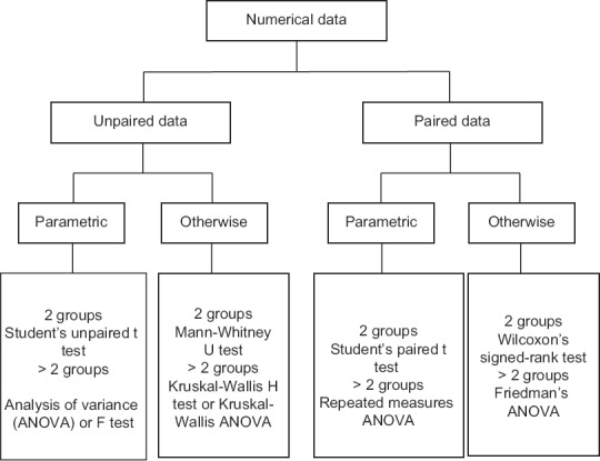
Statistical tests to compare numerical data for difference
Student's T-test
The Student's t-test is used to test the null hypothesis that there is no difference between two means. There are three variants:
One-sample t-test: To test if a sample mean (as an estimate of a population mean) differs significantly from the population mean. In other words, it is used to determine whether a sample comes from a population with a specific mean. The population mean is not always known, but may be hypothesized
Unpaired or independent samples t-test: To test if the means estimated for two independent samples differ significantly
Paired or related samples t-test: To test if the means of two dependent samples, or in other words two related data sets, differ significantly.
The test is named after the pseudonym Student of William Sealy Gossett who published his work in 1908 while he was an employee of the Guinness Breweries company in Dublin and company policy prevented him from using his real name. His t-test is used when the underlying assumptions of parametric tests are satisfied. However, it is robust enough to tolerate some deviation from these assumptions which can occur when small samples (say n <30) are being studied. Theoretically, the t-test can be used even when the samples are very small (n <10), so long as the variables are normally distributed within each group and the variances in the two groups are not too different.
The t-test is based on the t distribution calculated by Student. A sample from a population with a normal distribution is also normally distributed if the sample size is large. With smaller sample sizes, the likelihood of extreme values is greater, so the distribution “curve” is flatter and broader [Figure 3]. The t distribution, like the normal distribution, is also bell shaped, but has wider dispersion-this accommodates for the unreliability of the sample standard deviation as an estimate of the population standard deviation. There is a t distribution curve for any particular sample size and this is identified by denoting the t distribution at a given degree of freedom. Degree of freedom is equal to one less than the sample size and denotes the number of independent observations available. As the degree of freedom increases, the t distribution approaches the normal distribution. The table for the t distribution would show that as the degree of freedom increases, the value of t approaches 1.96 at a P value of 0.05. This is analogous to a normal distribution where 5% of values lie outside 1.96 standard deviations from the mean.
Figure 3.
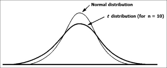
A t distribution (for n = 10) compared with a normal distribution. A t distribution is broader and flatter, such that 95% of observations lie within the range mean ± t × standard deviation (t = 2.23 for n = 10) compared with mean ± 1.96 standard deviation for the normal distribution
The formulae for the t-test (which are relatively simple) give a value of t. This is then referred to a t distribution table to obtain a P value. However, statistical software will directly return a P value from the calculated t value. To recapitulate, the P value quantifies the probability of obtaining a difference or change similar to the one observed, or one even more extreme, assuming the null hypothesis to be true. The null hypothesis of no difference can be rejected if the P value is less than the chosen value of the probability of Type I error (α), and it can be concluded that the means of the data sets are significantly different.
The unpaired t-test is used when two data sets that are “independent” of one another (that is values in one set are unlikely to be influenced by those in the other) are compared. However, if data sets are deliberately matched or paired in some way, then the paired t-test should be used. A common scenario that yields such paired data sets is when measurements are made on the same subjects before and after a treatment. Another is when subjects are matched in one or more characteristics during allocation to two different groups. A crossover study design also yields paired data sets for comparison. In the analysis of paired data, instead of considering the separate means of the two groups, the t-test looks at the differences between the two sets of measurements in each subject or each pair of subjects. By analyzing only the differences, the effect of variations that result from unequal baseline levels in individual subjects is reduced. Thus, a smaller sample size can be used in a paired design to achieve the same power as in an unpaired design.
If there is definite reason to look for a difference between means in only one direction (i.e., larger or smaller), then a one-tailed t-test can be used, rather than the more commonly used two-tailed t-test. This essentially doubles the chance of finding a significant difference. However, it is unfair to use a one-tailed t-test just because a two-tailed test failed to show P < 0.05. A one-tailed t-test should only be used if there is a valid reason for investigating a difference in only one direction. Ideally, this should be based on known effects of the treatment and be specified a priori in the study protocol.
Before we move on to comparison of more than two means, it is useful to take another view of the t-test procedure. Comparison of means of two samples essentially means comparing their central locations. When comparing central location between samples, we actually compare the difference (or variability) between samples with the variability within samples. Evidently, if the variability between sample means is very large and the variability within a sample is very low, a difference between the means is readily detected. Conversely if the difference between means is small but the variability within the samples is large, it will become more difficult to detect a difference. In the formula for the t-test, the difference between means is in the numerator. If this is small relative to the variance within the samples, which comes in the denominator, the resultant t value will be small and we are less likely to reject the null hypothesis. This effect is demonstrated in Figure 4.
Figure 4.
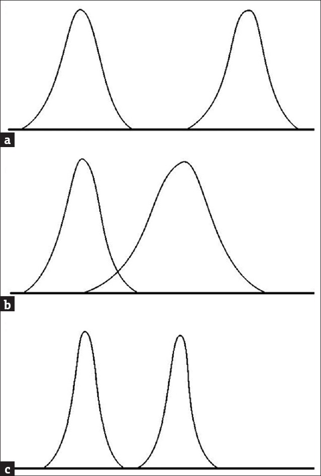
When comparing two groups, the ability to detect a difference between group means is affected by not only the absolute difference but also the group variance (a) two sampling distributions with no overlap and easily detected difference; (b) means now closer together causing overlap of curves and possibility of not detecting a difference; (c) means separated by same distance as in second case but the smaller variance means that there is no overlap, and the difference is easier to detect
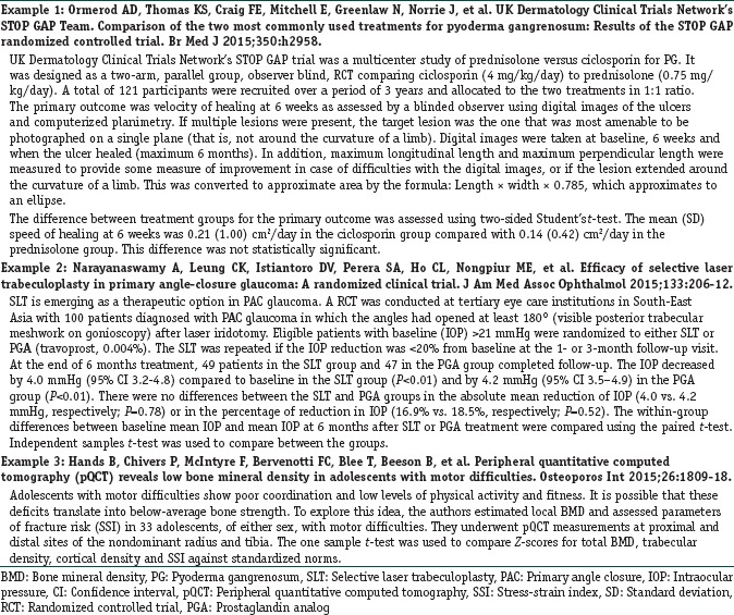
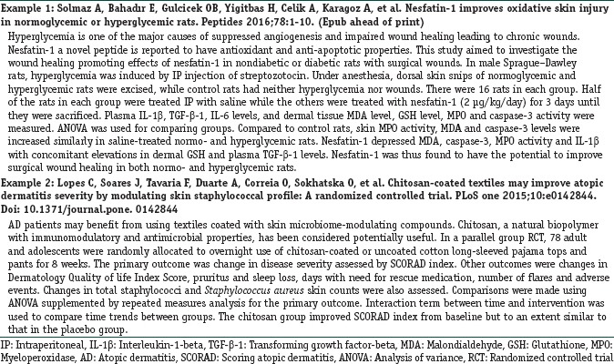
Box 1 provides some examples of t-test applications from published literature.
Box 1.
Examples of t-test applications from published literature
Comparing Means of More than Two Groups
The t-test should not be used to compare the means of three or more groups. Although it is possible to compare groups in pairs, when there are more than two groups, this will increase the probability of making a Type I error. For instance in an eight group study, there would be 28 possible pairs and with α of 0.05, or 1/20, there is every possibility that the observed difference in one of the pairs would occur by chance.
To circumvent the problem of inflated Type I error risk during multiple pair-wise testing, it has been proposed to divide the critical P value for each test by the total number of pair-wise comparisons, so that overall, the Type I error is limited to the original α. For example, if there are three t-tests to be done, then the critical value of 0.05 would be reduced to 0.0167 for each test and only if the P value is less than this adjusted α, would we reject the null hypothesis. This maintains a probability of 0.05 of making a Type I error overall. This principle is known as the Bonferroni correction (after Carlo Emilio Bonferroni). However, it is apparent that as the number of comparisons increases, the adjusted critical value of P becomes increasingly smaller, so that the chance of finding a significant difference becomes miniscule. Therefore, the Bonferroni correction is not universally accepted, and in any case, is considered to be untenable when more than 5 comparisons could be made, as it renders the critical value of P < 0.01.
The comparison of means of multiple groups is best carried out using a family of techniques broadly known as one-way analysis of variance (ANOVA). When conducting multiple comparisons, ANOVA is generally also more powerful, that is more efficient at detecting a true difference.
In biomedical literature, we sometimes come across a Z-test applied to situations where the t-test could have been used. The term actually refers to any statistical test for which the distribution of the test statistic under the null hypothesis can be approximated by a normal distribution. The test involves in the calculation of Z -score. For each significance level, the Z-test has a single critical value (e.g., 1.96 for two-tailed 5%) unlike the Student's t-test which has separate critical values for each sample size. Many statistical tests can be conveniently performed as approximate Z-tests if the sample size is large and the population variance is known. If the population variance is unknown (and therefore has to be estimated from the sample itself) and the sample size is not large (n < 30), the Student's t-test may be more appropriate.
A one-sample location test, two-sample location test, and paired difference test are examples of tests that can be conducted as Z-tests. The simplest Z-test is the one-sample location test that compares the mean of a set of measurements to a given population mean when the data are expected to have a common and known variance. The Z-test for single proportion is used to test a hypothesis on a specific value of the population proportion. The Z-test for difference of proportions is used to test the hypothesis that two populations have the same proportion. There are other applications such as determining whether predictor variables in logistic regression and probit analysis have a significant effect on the response and undertaking normal approximation for tests of poisson rates. These normal approximations are valid when the sample sizes and the number of events are large. A useful set of Z-test calculators can be found online at <http://in-silico.net/tools/statistics/ztest/>.
Analysis of Variance
ANOVA is employed to test for significant differences between the means of more than two groups. Thus, it may be regarded as a multiple group extension of the t-test. If applied to two groups, ANOVA will return a result similar to the t-test. ANOVA uses the same assumptions that apply to parametric tests in general.
Although it may seem strange that a test that compares means is called ANOVA, in ANOVA, we are actually comparing the ratio of two variances. We have already considered, in relation to the t-test, that a significant result is more likely when the difference between means is greater than the variance within the samples. With ANOVA, we also compare the difference between the means (using variance as our measure of dispersion) with the variance within the samples that results from random variation between the subjects within each group. The test asks if the difference between groups (between-group variability) can be explained by the degree of spread within a group (within-group variability). To answer this, it divides up the total variability into between group variance and within group variance and takes a ratio of the two. If the null hypothesis was true, the two variances will be similar, but if the observed variance between groups is greater than that within groups, then a significant difference of means is likely. The within-group variability is also known as the error variance or residual variance because it is variation we cannot readily account for in the study design since it stems from random differences in our samples. However, in a clinical trial situation, we hope that the between-group, or effect variance, is the result of our treatment.
From these two estimates of variance we compute the F statistic that underlies ANOVA. In a manner analogous to the t-test, the F statistic calculated from the samples is compared with known values of the F distribution, to obtain a P value. If this value is less than the preselected critical value of the probability of Type I error (α), then the null hypothesis of no difference between means can be rejected. However, it is important to note that if k represents the number of groups and n the total number of results for all groups, the variation between groups has degrees of freedom k − 1, and the variation within groups has degrees of freedom n − k. When looking at the F distribution table, the two degrees of freedom must be used to locate the correct entry. These complex manipulations are programmed into statistical software that provides ANOVA routines, and a P value is automatically returned.
If ANOVA returns P < 0.05, this only tells us that there is a significant difference but not exactly where (i.e., between which two groups) the difference lies. Thus, if we are comparing more than two samples, a significant result will not identify which sample mean is different from any other. If we are interested in knowing this, we must make use of further tests to identify where the differences lie. Such tests that follow a multiple group comparison test are called post hoc tests.
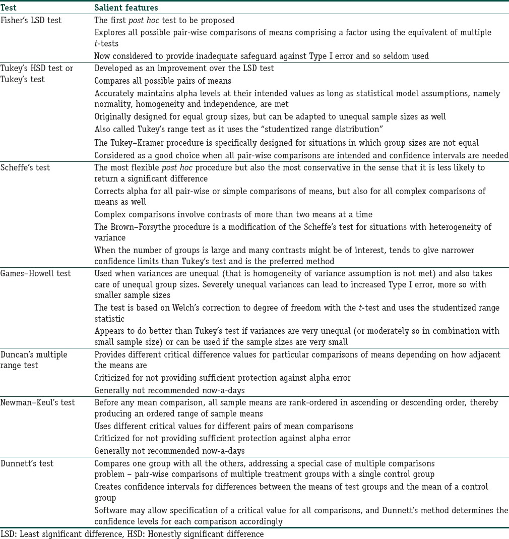
One confusing aspect of ANOVA is that there are many post hoc tests without consensus among statisticians as to which test should be used most commonly. The tests differ in the amount and kind of adjustment for alpha error provided. Statistical software packages offer choice of multiple post hoc tests. Tukey's (honestly significant difference) test (after John Wilder Tukey) is frequently used. Dunnett's test (after Charles William Dunnett) is used specifically when one wishes to compare all other means to the mean of one data set (the “control” group). Table 1 provides a summary of the post hoc tests used following ANOVA.
Table 1.
Post hoc tests that may be applied following analysis of variance
The advancement in statistical software permits use of ANOVA beyond its traditional role of comparing means of multiple groups. If we simply compare the means of three or more groups, the ANOVA is often referred to as a one-way ANOVA or one-factor ANOVA. There is also two-way ANOVA when two grouping factors are analyzed and multivariate ANOVA when multiple dependent variables are analyzed. An example of one-way ANOVA would be to compare the changes in blood pressure between groups after the administration of three different drugs. If we wish to look at one additional factor that influences the result, we can perform the two-way ANOVA. Thus, if we are interested in gender-specific effect on blood pressure, we can opt for a two-factor (drug treatment and gender) ANOVA. In such a case the ANOVA will return a P value for the difference based on drug treatment and another P value for the difference based on gender. There will also be P value for the interaction of drug treatment and gender, indicating perhaps that one drug treatment may be more likely to be effective in patients of a certain gender. As an extended statistical technique, ANOVA can test each factor while controlling for all other factors and also enable us to detect interaction effects between factors. Thus, more complex hypotheses can be tested, and this is another reason why ANOVA is considered more desirable than applying multiple t-tests.
Repeated measures ANOVA can be regarded as an extension of the paired t-test, used in situations where repeated measurements of the same variable are taken at different points in time (a time series) or under different conditions. Such situations are common in drug trials, but their analysis has certain complexities. Parametric tests based on the normal distribution assume that data sets being compared are independent. This is not the case in a repeated measures study design because the data from different time points or under different conditions come from the same subjects. This means the data sets are related, to account for which an additional assumption has to be introduced into the analysis. This is the assumption of sphericity which implies that the data should not only have the same variance at each time but also that the correlations between all pairs of repeated measurements should be equal. This is often not the case – in the typical repeated measures situation, values at adjacent time points are likely to be closer to one another than those further apart. The effect of violation of the sphericity assumption is loss of power, that is, the probability of Type II error is increased. Software may offer the Mauchly's test of sphericity which tests the hypothesis that the variances of the different conditions are equal. If Mauchly's test returns a significant P value we cannot rely on the F -statistics produced in the conventional manner. The Greenhouse-Geisser or Hunyh-Feldt correction factors are applied in this situation.
ANOVA is a powerful statistical technique and many complex analyses are possible. However, there are also many pitfalls, especially with repeated measures ANOVA. Assistance from an experienced statistician is highly desirable before making elaborate ANOVA analyses the basis for important clinical decisions. Box 2 provides two examples of ANOVA use from literature. The second example is more complicated, and readers can download and study the full paper for understanding it better.
Box 2.
Examples of analysis of variance applications from published literature
Nonparametric Tests
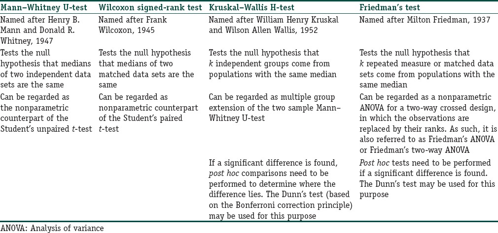
If the assumptions for the parametric tests are not met, there are many nonparametric alternatives for comparing data sets. Table 2 provides a summary.
Table 2.
Nonparametric tests commonly applied for assessing difference between numerical data sets
Nonparametric tests do not assume normality or some other underlying distribution and hence may be referred to as distribution-free tests. In addition to testing data that are known not to be normally distributed, they should be used for small samples where it is unlikely that the data can be demonstrated to be normally distributed. They do, however, have some underlying assumptions:
Data are at least on an ordinal scale
Observations within a group are independent of one another
The samples have been drawn randomly from the population.
Nonparametric tests convert the raw values into ranks and then perform calculations on these ranks to obtain a test statistic. The test statistic is then compared with known values for the sampling distribution of that statistic, and the null hypothesis is accepted or rejected. With these tests, the null hypothesis is that the samples come from populations with the same median. However, it is to be noted that, if applied to parametric data, nonparametric tests may fail to detect a significant difference where a parametric test may. In other words, they have less power to detect a statistically significant difference. Therefore, it is worthwhile to test for normality before finally selecting the test of significance to be applied.
Mann–whitney U-Test and Wilcoxon Rank Sum Test
The Mann–Whitney U-test is a distribution-free test used to determine whether two independent groups have been drawn from the same population. The test statistic U is calculated from comparing each pair of values, one from each group, scoring these pairs 1 or 0 depending on whether the first group observation is higher or lower than that from the second group and summing the resulting scores over all pairs. The calculated test statistic is then referred to the appropriate table of critical values to decide whether the null hypothesis of no difference in the location of the two data sets can be rejected. This test has fewer assumptions and can be more powerful than the t-test when conditions for the latter are not satisfied.
In the Wilcoxon rank sum test, data from both the groups are combined and treated as one large group. Then the data are ordered and given ranks, separated back into their original groups, and the ranks in each group are then added to give the test statistic for each group. Tied data are given the same rank, calculated as the mean rank of the tied observations. The test then determines whether or not the sum of ranks in one group is different from that in the other. This test essentially gives results identical to the more frequently used Mann–Whitney U-test.
Wilcoxon Signed-Rank Test
This test is considered as the nonparametric counterpart of the Student's paired t-test. It is named after Frank Wilcoxon, who, in a single paper in 1845, proposed both this test and the rank-sum test for two independent samples.
The test assumes data are paired and come from the same population. As with the paired t-test, the differences between pairs are calculated but then the absolute differences are ranked (without regard to whether they are positive or negative). The positive or negative signs of the original differences are preserved and assigned back to the corresponding ranks when calculating the test statistic. The sum of the positive ranks is compared with the sum of the negative ranks. The sums are expected to be equal if there is no difference between groups. The test statistic is designated as W.
Before the development of Wilcoxon matched pairs signed-rank test, the sign test was the statistical method used to check for consistent differences between pairs of observations. For comparisons of paired observations (designated x, y) the sign test is most useful if comparisons are only expressed as x > y, x = y, or x < y. If, instead, the observations can be expressed as numeric quantities (e.g., x = 7, y = 8), or as ranks (e.g., rank of x = 2nd, rank of y = 8th), then the Wilcoxon signed-rank test will usually have greater power than the sign test to detect consistent differences. If x and y are quantitative variables in the situation when we can draw paired samples, the sign test can be used to test the hypothesis that the difference between the median of x and the median of y is zero, assuming continuous distributions of the two variables x and y. The sign test can also assess if the median of a collection of numbers is significantly greater or lesser than a specified value.
Kruskal–Wallis Test
The Kruskal–Wallis test checks the null hypothesis that k independent groups come from populations with the same median. It is thus a multiple group extension of the two sample Mann–Whitney U-test.
Calculation of the test statistic H entails rank ordering of the data like other distribution-free tests. It is also referred to as the Kruskal–Wallis ANOVA because the calculation is analogous to the ANOVA of a one-way design.
If a significant difference is found between groups, post hoc comparisons need to be performed to determine where the difference lies. The Mann–Whitney U-test with a Bonferroni correction may be applied for this. Alternatively, the Dunn's test (named after Olive Dunn, 1964), which is also based on the Bonferroni correction principle, may be used.
Friedman's Test
Named after the Nobel Prize winning economist Milton Friedman, who introduced it in 1937, this tests the null hypothesis that k repeated measures or matched groups come from populations with the same median. It represents the distribution free counterpart of repeated measures ANOVA.
The test may be regarded as a nonparametric ANOVA for a two-way crossed design, in which the observations are replaced by their ranks. As such, it is also referred to as Friedman's two-way ANOVA or simply Friedman's ANOVA.
Post hoc tests need to be performed if a significant difference is found. The Dunn's test may be used for this purpose.
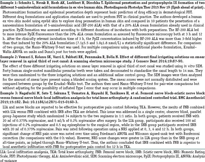
Box 3 provides some examples from literature of use of nonparametric tests.
Box 3.
Examples of nonparametric tests from published literature
Financial support and sponsorship
Nil.
Conflicts of interest
There are no conflicts of interest.
Further Reading
- 1.Pereira-Maxwell F. A-Z of Medical Statistics: A Companion for Critical Appraisal. London: Arnold (Hodder Headline Group); 1998. [Google Scholar]
- 2.Kirkwood BR, Sterne JA. Essential Medical Statistics. 2nd ed. Oxford: Blackwell Science; 2003. [Google Scholar]
- 3.Everitt BS. Medical Statistics from A to Z: A Guide for Clinicians and Medical Students. Cambridge: Cambridge University Press; 2006. [Google Scholar]
- 4.Miles PS. Statistical Methods for Anaesthesia and Intensive Care. Oxford: Butterworth-Heinemann; 2000. [Google Scholar]
- 5.Field A. Discovering Statistics Using SPSS. 3rd ed. London: SAGE Publications Ltd; 2009. [Google Scholar]