Developing EHR-driven Heart Failure Risk Prediction Models using CPXR(Log) with the Probabilistic Loss Function

Abstract

Computerized survival prediction in healthcare identifying the risk of disease mortality, helps healthcare providers to effectively manage their patients by providing appropriate treatment options. In this study, we propose to apply a classification algorithm, Contrast Pattern Aided Logistic Regression (CPXR(Log)) with the probabilistic loss function, to develop and validate prognostic risk models to predict 1, 2, and 5 year survival in heart failure (HF) using data from electronic health records (EHRs) at Mayo Clinic. The CPXR(Log) constructs a pattern aided logistic regression model defined by several patterns and corresponding local logistic regression models. One of the models generated by CPXR (Log) achieved an AUC and accuracy of 0.94 and 0.91, respectively, and significantly outperformed prognostic models reported in prior studies. Data extracted from EHRs allowed incorporation of patient co-morbidities into our models which helped improve the performance of the CPXR(Log) models (15.9% AUC improvement), although did not improve the accuracy of the models built by other classifiers. We also propose a probabilistic loss function to determine the large error and small error instances. The new loss function used in the algorithm outperforms other functions used in the previous studies by 1% improvement in the AUC. This study revealed that using EHR data to build prediction models can be very challenging using existing classification methods due to the high dimensionality and complexity of EHR data. The risk models developed by CPXR(Log) also reveal that HF is a highly heterogeneous disease, i.e., different subgroups of HF patients require different types of considerations with their diagnosis and treatment. Our risk models provided two valuable insights for application of predictive modeling techniques in biomedicine: Logistic risk models often make systematic prediction errors, and it is prudent to use subgroup based prediction models such as those given by CPXR(Log) when investigating heterogeneous diseases.

Graphical abstract

1. Introduction

Heart Failure (HF) is a major health issue and is one of the most common causes of hospitalization in the United States (US) with an estimated 6.6 million US adult cases in 2010 at a cost of 34.4 billion US dollars in healthcare expenses [1]. In the general population, the lifetime risk of subsequently developing HF in individuals initially free of the disease at the of age 40 years is 1 in 5 [2]. The high mortality rate in HF patients is a major public health care priority [3]. Identification of cost-effective strategies to reduce the incidence of hospitalization, a major driver of costs, is a major objective. Central to the management of HF is multifaceted pharmacological intervention that involves treatment of volume overload for symptom relief and disease modification in high risk patients to reduce mortality.

Accurate HF survival prediction models can be beneficial to both patients and physicians. Physicians could prescribe more aggressive treatment plans for high risk patients based on accurate risk predictions, and patients can have confidence in the treatment plan prescribed by physicians, and hence are more likely to comply with treatment. Accurate HF survival prediction models also help clinical researchers in designing clinical trials by targeting high risk patients with heterogeneous characteristics for disease modifying therapeutic interventions [4]. Multiple HF survival prediction models, such as the Seattle Heart Failure Model (SHFM) [5], [6], and [7], have been developed and validated in multiple cohorts and are being used in routine clinical care to manage HF patients with varying degrees of success and adoption [8]. However, there are two major limitations hindering the broad-scale adoption of such survival prediction models for HF: (1) These prognostic HF models were derived from clinical trials databases that represent a population of patients with limited generalizability (e.g., care provided in closely monitored settings in larger academic medical centers, smaller patient sample size, lack of heterogeneity in the patient population). Such models are not very useful for making accurate predictions in real-world community based settings [9]. (2) These clincial trial based models do not always include multiple co-morbid factors found in a real-world population that can be accurately derived from EHRs. Incorporating co-morbdities is important because the true value of prognostic models used for routine clinical care can only be achieved when prognostic models can facilitate (EHR-driven) clinical decision making at the bedside.

Consequently, with increasing availability of EHR data that allows tracking of real-world patient chracteristics and outcomes, it is imperative to develop and validate EHR derived survival prediction models for HF prognosis of patients seen in routine clincial practice instead of those derived from clinical trials databases. However, there are many challenges, at least from the modeling perspective, in developing purely EHR-driven risk prediction models. Some of these challenges include: (1) models need to be highly accurate with very few false positive cases; (2) models need to be highly interpretable [10] so that healthcare providers can apply them to identify clinically relevant prognostic markers, that allow them to make informed clinical decisions, and (3) the models need to minimize overfitting so that they are generalizable and can make accurate predictions on new cases.

To address these challenges, in this study, we apply the recently introduced CPXR(Log) method (Contrast Pattern Aided Logistic Regression) on HF survival prediction with the probabilistic loss function. CPXR(Log) is the classification adoption of CPXR, which was recently introduced in [11] by two of the current authors. The algorithm proposed in [11] involves prediction for numerical response variables, whereas CPXR(Log) involves classification for binary class labels. The CPXR(Log) method constructs a pattern aided logistic regression model defined by several patterns and corresponding local logistic regression models. CPXR(Log) has several significant advantages including

• CPXR(Log) builds highly accurate models, often outperforming standard logistic regression and state-of-the-art classifiers significantly on various accuracy measures.

• CPXR(Log) has the ability to handle data with diverse and heterogeneous predictor-response relationships.

• CPXR(Log) models are easy to interpret and are less overfitting when compared to other classifiers (see Table 6).

Table 6.

Odd ratios of CPXR(Log) for 1-year HF survival model

Odds Ratios in baseline and local models
Variable	Logistic Regression	f1	f2	f3	f4	f5	f6	f7	f8	f9	f10
Age	1.01	1.00	1.02	1.00	1.02	1.01	1.01	1.00	1.01	1.00	1.01
Sex (Male)	1.26	1.19	1.57	0.96	0.76	1.23	1.87	1.09	1.53	0.97	1.35
Race (White)	1.03	0.98	1.00	0.98	0.54	0.38	1.00	0.9	1.00	0.49	1.00
Ethnicity	0.4	0.42	0.33	0.34	0.66	1.00	0.44	0.35	0.40	1.00	0.31
BP	1.00	1.00	1.00	1.00	1.00	1.00	0.99	1.00	1.00	0.99	1.00
BMI	0.98	0.97	0.99	0.98	0.99	0.97	0.96	0.98	0.97	0.96	0.99
EF	0.99	1.00	1.00	0.99	0.99	0.99	1.00	1.00	1.00	0.99	1.00
Hemoglobin	0.91	0.95	0.94	1.00	1.00	1.08	0.94	0.95	0.95	1.03	0.96
Lymphocytes	1.01	1.02	1.06	1.00	1.01	0.99	1.08	1.03	1.02	1.03	1.00
Cholesterol	1.00	1.01	1.01	1.01	1.00	1.01	1.01	1.00	1.01	1.01	1.00
Sodium	1.00	1.00	0.99	1.00	1.00	1.00	0.99	1.00	1.00	1.00	1.00
ACE	0.65	0.77	0.63	0.84	0.71	0.61	0.93	0.64	0.72	0.77	0.61
β-blockers	0.86	0.93	1.19	0.84	0.76	1.00	0.95	0.9	1.04	1.00	1.00
ARB	1.16	1.15	1.74	1.16	1.16	0.97	1.48	1.73	1.07	1.28	1.05
CCB	1.44	1.78	2.22	1.78	1.53	2.12	1.00	2.13	1.00	1.00	3.05
Statins	1.02	0.94	0.85	0.81	0.88	1.30	0.96	1.00	1.07	1.24	1.08
Allopurinol	1.10	0.91	0.93	0.79	1.00	0.65	0.99	0.86	0.81	0.64	0.87
Diuretics	1.28	1.33	1.4	1.45	1.40	1.67	1.00	1.26	1.28	1.61	1.36
Ischemic heart disease	0.92	1.01	1.14	1.26	1.14	1.23	1.09	1.29	1.11	1.07	1.17
Alzheimer	1.75	1.74	0.80	1.88	1.59	1.29	1.58	0.75	1.00	1.79	0.51
Anemia	1.19	1.14	1.20	1.05	1.21	1.67	1.02	1.3	0.90	1.31	1.21
Arthritis	0.86	0.94	1.14	0.84	0.94	1.04	1.22	1.02	1.22	1.11	1.23
Asthma	0.75	0.65	0.51	0.52	0.45	0.60	0.72	0.99	1.00	0.63	0.51
Breast cancer	0.63	1.15	1.62	2.73	1.00	1.00	2.08	0.59	0.92	1.00	1.90
Cataract	0.74	0.97	0.92	0.90	1.22	0.89	0.86	1.15	1.0	1.04	1.13
Colorectal cancer	1.00	1.00	1.27	0.86	0.62	1.00	1.00	0.83	1.00	0.70	1.00
Depression	0.99	1.23	1.46	1.41	1.02	0.96	1.18	1.00	1.45	0.80	1.08
Diabetics	1.06	1.07	0.92	0.92	1.13	0.91	1.07	1.17	1.22	1.13	1.02
Atrial fibrillation	0.86	1.05	0.86	0.95	0.93	0.78	0.88	0.92	0.93	0.70	1.00
Glaucoma	1.13	1.18	1.34	1.22	1.34	1.58	1.32	1.51	1.89	1.00	1.78
Hip fracture	1.00	1.19	4.53	1.00	1.00	1.00	0.72	1.00	0.62	1.00	1.00
Hyperlipidemia	0.93	0.86	1.06	0.81	0.72	0.79	0.76	1.09	0.55	0.73	0.86
Hypertension	0.91	0.67	0.68	0.79	0.70	0.86	0.59	0.53	0.71	0.78	0.69
Hypothyroid	1.13	1.23	1.84	1.00	1.25	1.44	1.59	2.22	1.47	1.66	1.48
Kidney disease	1.41	1.40	1.06	2.14	1.32	1.83	1.51	1.17	1.68	1.68	1.28
Lung cancer	1.16	1.12	0.87	1.00	1.00	1.06	1.00	1.08	1.00	1.00	0.73
Myocardial infarction	1.34	1.27	1.00	1.24	1.44	0.8	1.00	1.51	1.05	0.71	1.31
Osteoporosis	1.3	1.36	1.15	1.03	1.52	1.00	1.67	1.00	1.48	1.61	1.00
Prostate cancer	0.48	0.39	1.00	0.67	0.69	1.00	0.34	0.51	0.59	0.44	0.31
Prostatic	0.6	0.61	0.56	0.35	0.78	0.53	0.63	0.60	0.72	1.22	0.44
Pulmonary embolism	1.03	1.22	0.76	1.45	1.11	1.20	0.73	0.88	0.98	1.05	1.24
Stroke	0.86	0.80	1.00	1.77	0.92	0.64	1.01	1.00	0.38	1.10	1.00

The ability to effectively handle data with diverse predictor-response relationships is especially useful in clinical applications, as modern medicine is becoming increasingly personalized, and the patient population for a given disease is often highly heterogeneous. As stated by President Obama when he announced the Precision Medicine Initiative [12]: “Most medical treatments have been designed for the average patient. As a result of this one-size-fits-all-approach, treatments can be very successful for some patients but not for others. This is changing with the emergence of precision medicine, an innovative approach to disease prevention and treatment that takes into account individual differences in people’s genes, environments, and lifestyles”. CPXR(Log) can effectively identify important disease subgroups from patients EHR data, and it can produce localized prediction models for “personalized” considerations for those subgroups. In prior studies, two of the current authors applied CPXR(Log) on outcome prediction for Traumatic Brain Injury (TBI) patients [13], where they obtained highly accurate prediction models and identified different patient subgroups that require different considerations for TBI. The main differences between the algorithm introduced in this study and [13] are the following: (1) A new probabilistic loss function is used to split instances into large error and small error classes. Our experimental results demonstrate that the new loss function returns more accurate models compared to methods introduced in [13]. (2) A new method is applied to select cutoff values in order to optimize accuracy, precision, and recall.

The major contributions of this work include:

• We demonstrate that CPXR(Log) is a powerful methodology for clinical prediction modeling for high dimensional complex medical data: It can

  • ○produce highly accurate models (One CPXR(Log) model achieved an AUC and accuracy of 0.94 and 0.91, respectively, significantly outperforming models reported in prior studies), and
  • ○help to identify and correct significant systematic errors of logistic regression models.

• We present classification models for HF which are much more accurate than logistic models and models produced by other state-of-the-art classifiers.

• Our CPXR(Log) models for HF reveal that HF is highly heterogeneous, suggesting that patients with heterogeneous characteristics (e.g, clincial characteristics, co-morbidities) should be evaluated for different HF management strategies.

• We propose a novel probabilistic loss function in the CPXR(Log) algorithm. It returns more accurate models comparing to CPXR(Log) introduced in our previous studies.

The subsequent sections are organized as follows: In the next section, key related studies will be presented. In the materials and methods section, details of the Mayo Clinic EHR data for HF will be presented, and the CPXR(Log) algorithm will be explained. The experimental result section will report the prediction models produced by CPXR(Log) and other classification algorithms, together with an analysis of those models and discussions on various implications for the field of medicine. Finally, we will provide an overall summary in the conclusion section. The Mayo Clinic IRB approved this observational study.

2. Related Work

Studies related to our work can be categorized into three main groups:

1. Studies on general prediction models using EHR data: clinical prediction modeling is a very broad area of research. Logistic regression [14] is the most popular method in clinical prediction modeling. Most recently different machine learning methods such as Random Forest (RF), Support Vector Machine (SVM) and AdaBoost have been used in clinical prediction modeling. Kennedy et al. [15] applied Random Forest to predict the probability of depression after Traumatic Brain Injury (TBI) diagnosis in a rehabilitation setting. In [16], Wei et al. applied SVM on a dataset from National Health and Nutrition Examination Survey (NHANES) to classify diagnosed diabetes patients from pre-diabetes and the reported AUC is 0.83. In a similar study, Wu et al. [17] used EHR data to develop a model to detect heart failure within 6 months before the actual HF diagnosis. They compared the performance of logistic regression, SVM and Boosting, and SVM had the poorest performance. Lack of balance in class distribution and difficulty to define patient’s outcome are two EHR related challenges reported by Wu et al. Similarly, Zupan et al. [18] proposed a method to adopt machine learning techniques to handle censored data. They applied their algorithm to predict the recurrence of prostate cancer and compared the performance of Naïve Bayes, Decision Tree, and Cox regression.

   There are also some studies that used clustering techniques to identify subgroups of heart failure patients. Hertzong et al. [19] used hierarchical clustering to derive 3 clusters based on 14 symptoms. In another study, Song et al. [20] also applied agglomerative hierarchal clustering with Ward’s method to explore which physical symptom clusters occur in HF patients and to determine the impact of symptom clusters on event-free survival.

   There are some substantial differences between the CPXR methodologies and clustering based methodologies. CPXR(Log) models are easier to understand as each subgroup of a CPXR(Log) model is described by a pattern (which is a simple condition involving a small number of variables); in contrast the subgroups (clusters) obtained by clustering methods do not have natural discriminative descriptions other than cluster means. Secondly, Clustering methods are typically based on distance functions where the features are usually treated as equally important, but in practice, not all features are equally important. CPXR(Log) uses contrast mining algorithms to extract the most informative interactions between predictor variables and response variable and utilize them to build accurate prediction models.

2. Studies on HF survival prediction models: The Seattle Heart Failure Model (SHFM) is a well known HF risk model. It was derived from a cohort of 1125 HF patients from the PRAISE I clinical trial using a multivariate Cox model [21]. The model has been prospectively validated in 5 other cohorts totaling 9942 heart failure patients and 17307 person-years of follow-up. In addition to SHFM, several other risk prediction models have been developed including SHOCKED, Frankenstein, PACE Risk Score, and HFSS [7]; these 4 models were validated in independent cohorts along with SHFM. The Heart Failure Survival Score (HFSS) was validated in 8 cohorts (2240 patients), showing poor-to-modest accuracy (AUC, 0.56–0.79); the score is lower in more recent cohorts. In [2], Ouwerkerk et al. compared the performance of 117 HF models with 249 different variables. They concluded that clinical trial based models have lower performance compared to EHR based models.

   Furthermore, there are studies that applied machine learning algorithms to study risk factors and predict patient outcomes in HF. For example, Dai et al. [22] used boosting and SVM to build models to predict heart failure around 6 months before the actual diagnosis. Their results show that SVM has poor performance. Similarly, Panahiazar et al. [23] used decision tree, Random Forest, AdaBoost, SVM and logistic regression to predict survival risk of HF patients. They concluded that logistic regression generates more accurate models.

3. Studies on applying CPXR methodology: There are two studies that applied CPXR method. In [13], we applied CPXR(Log) to predict patient outcomes with Traumatic Brain Injury (TBI) within 6 months after the injury using admission time data. CPXR achieved AUC as high as 0.93. In [24], Ghanbarian et al. used CPXR to predict Saturated Hydraulic Conductivity, and the R² of their models was 0.98. Another advantage of this method was that the effect of sample size on the performance that was not detectable by linear regression.

3. Materials and Methods

3.1. Study population

Our primary goal in this study is to develop classifiers to predict survival in 1-, 2- and 5- years after HF diagnosis. Our classifiers are built using EHR data on 119,749 patients admitted to Mayo Clinic between 1993 and 2013. Some patient records (N=842) were excluded due to incomplete and missing data. In consultation with cardiologists and cardiovascular epidemiologists, the following cohort identification criteria were developed:

• A diagnosis of HF based on the ICD9-CM code (428.x).

• An EF measurement of ≤50% within two months of HF diagnoses.

• No prior diagnosis of coronary artery disease, myocarditis, infiltrative cardiomyopathy and severe valvular disease.

• Authorization to access EHR data for research.

To be included in this cohort, patients needed to meet all four criteria, leading to a final cohort size of 5044 HF patients admitted to Mayo Clinic between 1993 and 2013. To select predictor variables, we followed the SHFM [2] and added a series of new variables derived from the EHR data that were grouped into the following categories:

• Demographics including age, gender, race, and ethnicity.

• Vitals including Blood Pressure (BP), and Body Mass Index (BMI).

• Lab results including cholesterol, sodium, hemoglobin, lymphocytes, and ejection fraction (EF) measurements.

• Medications including Angiotensin Converting Enzyme (ACE) inhibitors, Angiotensin Receptor Blockers (ARBs), β-adrenoceptor antagonists (β-blockers), Statins, Calcium Channel Blocker (CCB), Diuretics, Allopurinol, and Aldosterone blocker.

• A list of 24 major chronic conditions [25] as co-morbidities including Acquired hypothyroidism, Acute myocardial infarction, Alzheimer, Anemia, Asthma, Atrial fibrillation, Benign prostatic hyperplasia, Breast cancer, Cataract, Chronic kidney disease, Colorectal cancer, Depression, Diabetes, Glaucoma, Hip/pelvic fracture, Hyperlipidemia, Hypertension, Ischemic heart disease, Lung cancer, Osteoporosis, Prostate cancer, Pulmonary disease, Rheumatoid arthritis, and Stroke.

Since our EHR data is time dependent, we considered the records that are closest to the HF event. Our class variable (response) is mortality status. For the 1-year version of the dataset, if a patient was dead within 1-year after the heart failure event, the class variable is 1, otherwise it is 0. We created 3-year and 5-year versions of the dataset similarly.

Table 1 represents demographics, vitals and lab characteristics of patients in our cohort, and Table 2 shows frequencies of co-morbidities. It can be observed that hypertension, ischemic heart disease, hyperlipidemia, chronic kidney disease and atrial fibrillation are the most frequent co-morbidities. Table 3 represents the frequency of different medication classes used in the cohort; apparently ACE inhibitors, β-blockers, and diuretics are the most popular medications used to treat heart failure.

Table 1.

Clinical characteristics of patients in the Mayo Clinic EHR-derived heart failure cohort

Age (in years)	78±10
Sex (male)	52%
Race (White)	94%
Ethnicity (Not Hispanic or Latino)	84%
BMI	28.7±11.25
Systolic Blood Pressure (mm/Hg)	120±25
Ejection Fraction (EF %)	36%±10.3
Hemoglobin (g/dL)	11.8±1.2
Cholesterol (mg/dL)	144±35
Sodium (mEq/L)	128±4.2
Lymphocytes (×10(9)/L)	1.32±0.7

Table 2.

Frequency of co-morbidities in the Mayo Clinic EHR-derived heart failure cohort

Co-morbidities	Frequency (N=5044)
Acquired hypothyroidism	21.20%
Acute myocardial infarction	16.30%
Alzheimer	11.90%
Anemia	53.01%
Asthma	10.72%
Atrial fibrillation	48.56%
Benign prostatic hyperplasia	9.50%
Cataract	31.40%
Chronic Kidney Disease	55.83%
Pulmonary disease	30.40%
Depression	25.50%
Diabetes	37.40%
Glaucoma	9.40%
Hip/pelvic fracture	4.30%
Hyperlipidemia	64.30%
Hypertension	81.06%
Ischemic heart disease	70.20%
Osteoporosis	18.30%
Rheumatoid Arthritis	39.20%
Stroke	12.40%
Breast cancer	2.20%
Colorectal cancer	1.58%
Prostate cancer	4.50%
Lung cancer	2.45%

Table 3.

Frequency of medication classes in the EHR-derived Mayo Clinic heart failure cohort

Medication class	Frequency (N=5044)
ACE inhibitor	55.7%
B blocker	48.6%
Angiotensin Receptor Blocker	12.8%
Calcium Channel Blocker	4.1%
STATIN use	43.2%
Diuretic use	68.7%
Allopurinol use	18.5%
Aldosterone Blocker	18.5%

Out of a total of 43 predictor variables, there are 35 binary predictor variables, which include race, ethnicity, gender, and all co-morbidities and medications, and there are 8 numerical variables, including lab results, age, BP, BMI and, EF measurement.

In the next section, we first discuss about preliminaries required by CPXR(Log) and then the CPXR(Log) algorithm will be presented.

3.2. The CPXR(Log) Algorithm

Preliminaries

Let D be a training dataset. A pattern is a finite set of single-variable conditions in one of two forms: (1) “A=a” where a is a constant, if A is a categorical variable, (2) “v₁ ≤ A <v₂”, where v₁ and v₂ are constants, if A is numerical. For us, the numerical constants are usually the bin boundaries produced when discretizing numerical variables using the entropy-based method [26]. A data instance X is said to satisfy, or match, a pattern P if X satisfies every condition in P. The matching dataset of P within a dataset D is mds(P,D) = {X∈D | X matches P}. The support of P in D is $\text{supp}(\mathrm{P},\mathrm{D})=\frac{\left|\text{mds}\right(\mathrm{P},\mathrm{D}\left)\right|}{\left|\mathrm{D}\right|}$.

Definition

Given two classes C₁ and C₂, the support ratio of P from C₁ to C₂ is $\mathbf{\text{suppRati}}{\mathbf{o}}_{{\mathbf{C}}_{\mathbf{1}}}^{{\mathbf{C}}_{\mathbf{2}}}(\mathbf{P})=\frac{\mathbf{supp}(\mathbf{P},{\mathbf{C}}_{\mathbf{2}})}{\mathbf{supp}(\mathbf{P},{\mathbf{C}}_{\mathbf{1}})}$. Given a support ratio threshold γ, a contrast/emerging pattern[27] of class C₂ is a pattern P satisfying $\mathbf{suppRati}{\mathbf{o}}_{{\mathbf{C}}_{\mathbf{1}}}^{{\mathbf{C}}_{\mathbf{2}}}(\mathbf{P})\ge \mathbf{\gamma }$. Thus, a pattern is a contrast pattern if its supports in different classes are very different. We may use a minSupp threshold, to limit contrast patterns to those P satisfying supp(P,C₂) ≥ minSupp.

3.2.1. CPXR(Log) concepts

This section presents the main ideas of the CPXR(Log) algorithm. More details can be found in [11] and [13]. We will also discuss our new contribution to the alogorithm where we measure errors in a probabilistic manner. Let D = {(X_i, Y_i)|1 ≤ i ≤ n} be a given training dataset for regression. Let f be a regression model built on D, which we will call the baseline model.

The main idea of CPXR is to use a pattern as logical characterization of a subgroup of data, and a regression model called local model as a behavioral characterization of the predictor-response relationship for data instances of that subgroup of data. CPXR is a powerful method, because it can pair a pattern and a local regression model to represent a specific predictor-response relationship for a subgroup of data and it has the flexibility in pairing multiple patterns and local regression models to represent diverse and distinct predictor-response relationships for multiple subgroups of data.

Definition

A pattern aided regression (PXR) model is represented by a tuple PM = ((P_i,f_i,w_i),…,(P_k,f_k,w_k), f_d) where, for each i, P_i (i=1,…,k) is a pattern, f_i (i = 1,…,k) is P_i′s local regression model, and is w_i ≥ 0 (i = 1,…,k) is f_i′s weight; f_d is the default model. The regression function of PM is defined (for each instance X) by

$$f(X)=\{\begin{array}{rr}\hfill \frac{{\displaystyle {\sum }_{P_i\in {\pi }_x}{w}_i{f}_i(X)}}{{\displaystyle {\sum }_{P_i\in {\pi }_x}{w}_i}},& \hfill if{\pi }_X\ne \text{Ø}\\ \hfill f_d(X),& \hfill \mathit{otherwise}\end{array},$$ (1)

where π_X = {P_i|1≤ i ≤ k, X satisfies P_i}.

Remark

f_i is applied on instances satisfying pattern P_i; f_d is used on instances not satisfying any pattern in PM.

In this study, we use standard logistic regression to build local regression models f_i. Standard logistic regression is a simple method producing interpretable models which have been used extensively in the field of biomedicine and bioinformatics [6].

Since the number of extracted patterns is huge and we want to have a small set of patterns with higher accuracy, it is necessary to define quality measures to remove patterns which reduce the overall accuracy of the models generated.

Let r_X(g) denote a function g’s residual on an instance X. The residual of logit function g on an instance X is the difference between the predicted and observed binary outcome variable values. The predicted outcome variable value of logit function is in the form of probability and is bounded to zero and one.

Definition

The average residual reduction (arr) of a pattern w.r.t. a prediction model f and a dataset D is

$$\mathit{arr}(P)=\frac{{\sum }_{X\in \mathit{mds}(P)}|r_X(f)|-{\sum }_{X\in \mathit{mds}(P)}|r_X(f_P)|}{|\mathit{mds}(P)|}$$ (2)

and the total residual reduction (trr) of a pattern set PS = {P₁,…P_k} w.r.t. to a prediction model f and a dataset D is:

$$\mathit{trr}(PS)=\frac{{\sum }_{X\in \mathit{mds}(PS)}|r_X(f)|-{\sum }_{X\in \mathit{mds}(PS)}|r_X(f_{PM})|}{{\sum }_{X\in D}|r_X(f)|}$$ (3)

where PM = ((P_i,f_i,w_i),…,(P_k,f_k,w_k), f), w_i = arr(P_i), mds(PS) = ∪_P∈PS mds(P).

We use arr to remove those patterns with little positive impact on the accuracy or those patterns that do not reduce the residual error. trr is used to measure how much a pattern set can reduce the residual error of the baseline model. Since some instances match more than one pattern, we need to use (1) to calculate the response (outcome) variable values.

3.2.2. Description of the CPXR(Log) algorithm

In this section, we explain the process of the CPXR(Log) algorithm. Readers can refer to [11] and [13] for more details on the algorithm. An outline of the CPXR(Log) algorithm is the following:

• Input: Training dataset D, ρ and minSup.

• Step 1: Train a baseline model on dataset D and calculate the residual error for each training instances using a loss function.

• Step 2: Split D into LE and SE using a splitting point cutr.

• Step 3: Discretize numerical predictor variables into bins using the equi-width or entropy binning method.

• Step 4: Mine contrast patterns of the LE dataset.

• Step 5: Perform a set of filtering methods to remove patterns that are highly similar to others or are not very generalizable (to avoid overfitting).

• Step 6: Train local models for the remaining patterns.

• Step 7: Remove patterns of low utility.

• Step 8: Select an optimal set of patterns, PS = {P₁,…P_k} with the highest trr.

• Step 9: Determine arr and local model f_P associated to each pattern in PS (to be used as weightes of local models).

• Step 10: Train the default model f_d.

• Output: A set of patterns associated with local models, weights, and default model; PXR = ((P₁,f₁,w₁), …,((P_k,f_k,w_k), f_d).

The CPXR(Log) algorithm has three inputs: a training dataset D, a ratio ρ to split dataset into large error (LE) and small error (SE) instances and a minSup threshold on the support of contrast patterns.

In the first step, CPXR(Log) builds a standard regression model f, called the baseline model, using a standard regression model. The model f returns a residual error for each instance X in dataset D. The residual error is calculated using a loss function. Then we use a parameter ρ to find a splitting point cutr (on residuals) to divide D into LE (large error) and SE (small error); we define $\rho =\frac{{\sum }_{X\in LE}|r_X(f)|}{{\sum }_{X\in D}|r_X(f)|}$. Then we have a dataset with two classes LE and SE. LE instances have large residuals (≥cutr) and SE instances have small residuals (< cutr) based on the baseline model f. Then the algorithm mines all contrast patterns of LE. These contrast patterns are more frequent on LE instances and less frequent on SE instances. Subsequently, filters are applied to remove some patterns with highly similar matching datasets.

In the next step, a local model f_P is built corresponding to each remaining contrast patterns. Some of these patterns do not improve the accuracy or have a small residual reduction. We use arr to identify and remove those patterns. Then the algorithm uses a double loop to search for a desirable pattern set with large trr. The inner loop performs repeated pattern replacements, and the outer loop adds a new pattern to the pattern set and then calls the inner loop. The inner loop terminates when the improvement of the best replacement is smaller than a threshold. The outer loop terminates when the improvement of the previous iteration is too small. The output of CPXR(Log) is a set of patterns PS = {P₁,…P_k}, a set of associated local standard regression models $f_{P_1},\cdots ,f_{P_k}$ for patterns in PS and arr(P₁),…,arr(P_k). arrs will be used when a new test case is matched with more than one pattern in PS. The algorithm also builds a logistic regression model f_d for the set of instances that do not match any pattern in PS.

3.2.3: The CPXR(Log) algorithm: new techniques and advancements

This section describes some new techniques and advancements introduced in the CPXR(Log) algorithm that were not used in previous studies involving CPXR and CPXR(Log).

The loss function is a key part of the CPXR(Log) algorithm, which is needed to measure classification errors on individual data instances. We now present three methods to measure classification error. Let h be a classifier, x be a data instance and y be the response variable of data instance x. In the first option h is assumed to return a class label and in the other two options h is assumed to return a probalility (of x being in one fixed class, e.g., the positive class).

• The binary error measure is defined by

  $$er{r}_b(h,x)=\{\begin{array}{cc}1,& ifh(x)=y\\ 0,& \mathit{otherwise}\end{array}$$
• The probabilistic error measure is defined by

  $$er{r}_p(h,x)=|y-h(x)|$$
• The Pearson residual error (standardized) is defined by

  $$er{r}_s(h,x)=\frac{|y-h(x)|}{\sqrt{h(x)(1-h(x))}}$$

Pearson residual error is a well-known formula used to measure the goodness of fit for logistic regression models and it was used in [13]. In this study, we evaluated the above functions, and our results suggest that probabilistic loss function returns more accurate models (see details in Section 4).

We also consider how to select the cutoff value in order to optimize accuracy, precision, and recall. The default cutoff value is usually 0.5 (if the predicted value is larger than 0.5, then the predicted class is 1, otherwise the predicted class is 0). In some experiments, we observed that 0.5 is not an optimal cutoff value for classification of the instances. Looking deeper at the predicted probabilities, we observed that, in some datasets, there are many false positive instances with the predicted probabilities close to 0.5 or there are many false negative instances with the predicted probabilities close to 0.5. To solve this problem, we designed the following simple method to find the optimal cutoff values: After CPXR(Log) returns a PXR model, we evaluate different cutoff values ranging from 0.3 to 0.8 on the training data; for each potential cutoff value, we calculate accuracy × precision × recall on the training data; the cutoff value that yields the optimal accuracy × precision × recall is chosen as the final cutoff value. This final cutoff value is used to classify new data instances, including to measure accuracy, precision and recall on the testing data.

4. Results and Discussions

This section presents the results of CPXR(Log) on HF risk prediction models, which are focused on four main aspects: (1) We compare the performance of CPXR(Log) against state-of-the-art classification algorithms such as Logistic Regression, Decision Tree, Support Vector Machine, Random Forest and AdaBoost. The results show that CPXR(Log) is much more accurate and outperforms other classifiers significantly. (2) We also present details on patterns and local models found by CPXR(Log) for HF risk prediction. Each pattern and the corresponding local model extracted by CPXR(Log) represent a distinct subgroup of patients with specific behaviors, whose survival risk should be calculated based on the local model assigned specifically to that subgroup of patients. Distinct pairs of patterns and local models are highly different from each other and they are highly different from the baseline model. (3) We show that the incorporation of co-morbidities extracted from EHR into our models improves the accuracy of CPXR(Log) and gives us more insights about the complexity of heart failure. We also show that the predictive power of co-morbidities has not been fully utilized by other classification algorithms – in fact those algorithms produced less accurate prediction models when they use the co-morbidities as features for modeling building. (4) We examine the effect of the probabilistic loss function and compare it with the loss function used in [13].

CPXR(Log) depends on two parameters, minSup and ρ. In this study, we used fixed parameter values (minSup = 0.03 and ρ = 0.45). Regarding the other classifiers, we used their implementation in standard R packages [28] Note that there are patient records with missing values for certain lab results and blood pressure measurements, a characteristic typical for real-world EHR data. We used multiple imputation to handle those missing values using a package called mi in R [29].

As explained earlier our problem is classifying patients who survived after a diagnosis of HF vs those who did not survive using the CPXR(Log) algorithm based on EHR data. Hence, our outcome (response) variable is mortality status. In this study, we developed and validated three models to predict 1-, 2-, and 5- years survival in HF patients with the use of EHR extracted variables including demographic, vitals, lab results, medications, and co-morbidities.

To enhance the generalizability of CPXR(Log) models, following common practice in clinical prediction modeling, we divide our dataset into two separate parts: a training part and a test part; the training dataset contains data for 1560 out of the 5044 patients, and the test dataset contains data for the remaining 3484 patients. The training and test datasets do not overlap.

We now compare the performance of CPXR(Log) against standard logistic regression and state-of-the-art classifiers concerning accuracy. Table 4 presents the AUC of the three models built by different classification algorithms. The results show that CPXR(Log) outperforms other classifiers consistently by large margins. The strong performance of CPXR(Log) implies there are highly diverse predictor-response relationships for HF patients and they were successfully extracted by CPXR(Log).

Table 4.

AUC of different classifiers for HF risk prediction using EHR-derived Mayo Clinic cohort

Algorithm	1 year	2 years	5 years
Decision Tree	0.66	0.5	0.5
Random Forest	0.8	0.72	0.72
Ada boost	0.74	0.71	0.68
SVM	0.59	0.52	0.52
Logistic Regression	0.81	0.74	0.73
CPXR(Log)	0.937	0.83	0.786

Furthermore, all CPXR(Log) models outperformed corresponding logistic regression and SVM models on all three other performance measures, as shown in Table 5. In Table 5, the cutoff values to optimize accuracy, precision and recall are determined in the way described in the previous section. In particular, CPXR(Log) improved the AUC of logistic regression, SVM, Random Forest and AdaBoost models by 15.6%, 58.8%, 17.1% and 26.6% on average, respectively. Further, Figures 1, 2 and 3 show that the ROC curves of all three CPXR(Log) models have larger true positive rate for every false positive rate, than that of logistic regression and SVM models. Our results are also better than those reported by prior from Levy et al. [5]. Specifically, the AUC of 1- year model developed by CPXR(Log) is 5.6% larger than the most accurate model developed by Levy et al. [5].

Table 5.

Precision, recall, and accuracy of different classifiers

Measure	Model	SVM	Log Reg.	CPXR (Log)
	1 year	0.66	0.752	0.82
Precision	2 Years	0.42	0.703	0.78
	5 years	0.2	0.513	0.721
	1 year	0.7	0.66	0.782
Recall	2 Years	0.68	0.643	0.76
	5 years	0.5	0.506	0.615
	1 year	0.75	0.89	0.914
Accuracy	2 Years	0.55	0.758	0.83
	5 years	0.66	0.717	0.809

Figure 1.

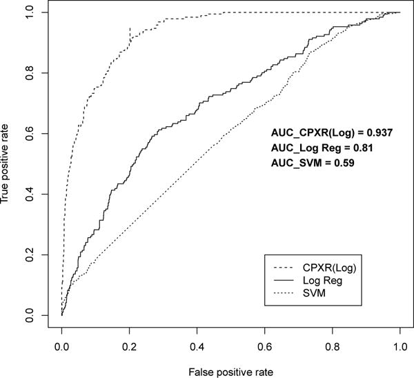
ROC curves for one year models

Figure 2.

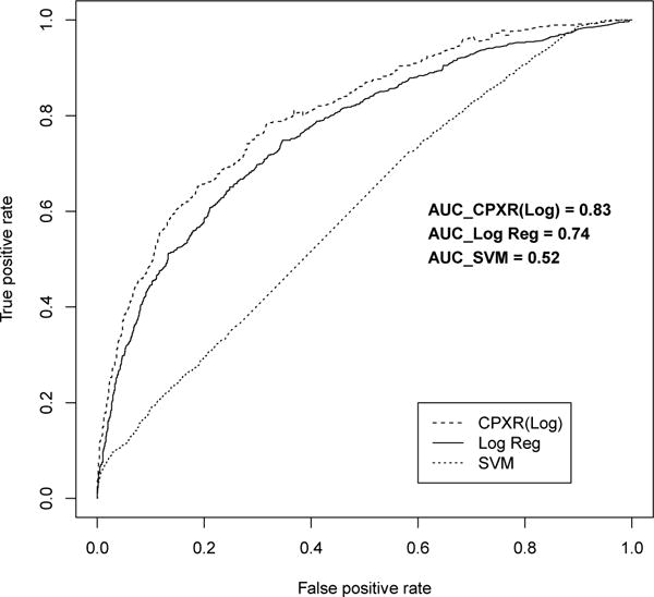
ROC curve for two year models

Figure 3.

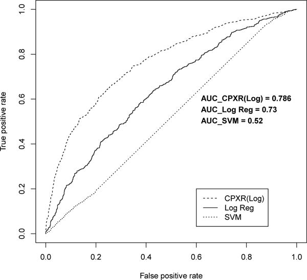
ROC curve for five year models

Next we present the CPXR(Log) patterns and models. Table 7 represents CPXR(Log) patterns and the odds ratios according to CPXR(Log) shown in Table 6. If a patient’s data matches any of the patterns listed in Table 7, then we should not follow the baseline model built for the whole population. Instead, to measure the survival risk, we should use the local model built specifically for the subgroup of patients associated with the matched pattern. The last column of Table 7 shows which model should be used to calculate the risk for which pattern. For example, according to pattern P₉, if a patient has a history of stroke, then the patient should be evaluated using model 9 (f₉) concerning his/her mortality risk. The 4^th column of Table 7 represents the coverage or support for each pattern in the training dataset.

Table 7.

Details on CPXR(Log) patterns

ID	Pattern	arr	Coverage	Model
P1	History of Asthma AND without history of Glaucoma	0.0007	10.6%	f1
P2	Age < 40 AND Cholesterol > 230 (mg/dL) AND EF =< 35 AND history of diabetes AND history of atrial fibrillation AND without history of Alzheimer	0.0021	6.2%	f2
P3	History of diabetes AND History of ARB use	0.0022	19.7%	f3
P4	Ethnicity = white AND history of kidney disease	0.0024	11.9%	f4
P5	History of CCB use AND history of Alzheimer	0.0022	8.7%	f5
P6	History of asthma AND without history of glaucoma	0.0021	10.5%	f6
P7	Lymphocyte < 2.4 (mg/dL) AND history of Alzheimer AND history of myocardial infarction	0.0014	3.6%	f7
P8	BP >= 130 AND history of pulmonary embolism	0.0018	21.8%	f8
P9	History of lung cancer AND history of ARB use	0.0027	5.3%	f9
P10	History of hypothyroid	0.0009	16.1%	f10

As we said earlier, Table 6 gives the odds ratios of variables, according to the local models of the 1-year CPXR(Log) model and the baseline model. (f_i is the local model of pattern i). Large differences in odds ratio between the baseline model and the CPXR(Log) local models can be of interest to physicians, as they indicate that for certain large population groups, survival risk should be evaluated in a manner different from how the risk is evaluated based on the standard logistic regression model for the whole patient population. Due to the popularity of logistic regression, one can assume that physicians are familiar with logistic regression models and they may have been using the information implied by such models in practice.

In Table 6, we use bold to indicate cases where odds ratio based on CPXR(Log) models is significantly higher or lower than that based on the standard logistic regression model (by at least 30% relative difference). There are quite a number of variables and value pairs where odds ratio differences are much larger. For example, the odds ratio for depression is 0.99 based on the baseline model, which says that if a patient has been diagnosed with depression within 3 years before the HF event, depression almost does not have any effect on increasing or decreasing the survival risk. However, if the patient’s data matches pattern 2 from Table 7, the odds ratio for depression is 1.46, making depression a very significant risk factor. We also highlight to indicate cases where the odds ratio changed from larger than one (positive effect) to smaller than one (negative effect). For example, the odds ratio of breast cancer according to the baseline model is 0.63, which says that if a patient has been diagnosed with breast cancer within 3 years before the HF event, the risk of death decreases. However, if a patient matches any of patterns 1, 2, 3, 6 or, 10 from Table 7, the risk of death increases. The above shows that local models can be different from the baseline model concerning both the positive and negative effects on the response variable.

Another interesting aspect of CPXR(Log) models is that they help identify diversity and heterogeneity of subgroups of HF patients. CPXR(Log) models are not only significantly different from the standard logistic regression model but also they are different from each other; such differences indicate that each (pattern, model) pair represents a distinct subgroup of patients with different behavior. For example, patterns 1 and 2 do not share any item with each other, and their odds ratios are significantly different in some of the predictor variables such as β-blockers use and Alzheimer disease.

We now give a concrete example where CPXR(Log) corrected a large prediction error observed in the baseline model. This is regarding a 39 years old male patient who was diagnosed with HF with a previous history of hypertension, but blood tests are normal. Since the patient is young and does not have abnormal lab results, the effect of hypertension is downgraded by SHFM [5] and the logistic model, and the risk of death is estimated at 38% and 47% by SHFM and logistic regression model, respectively. However, the observed outcome is that the patient deceased within one year after the HF event. We also had additional information about the patient that was not considered (or may have been ignored) by the other models. The EHR data indicate that the patient had a history of hip replacement surgery and had been diagnosed with pulmonary embolism. Many studies have found that hip and knee arthroplasty have high impact on the risk of pulmonary embolism [30]. This patient matches pattern 6 (BP >= 130 AND history of pulmonary embolism) of our CPXR(Log) model which includes patient co-morbidities, and the mortality risk is estimated to be 58% by the local model associated with pattern 6 – much higher compared to what was observed using SHFM and standard logistic regression. This example illustrates heterogeneity in HF, and highlights that co-morbidities play an important role in making accurate predictions of patients’ outcomes.

We now use our experimental results to discuss and highlight one of the main strengths of CPXR(Log), namely its ability to effectively utilize more predictor variables to derive more accurate models (a fact also observed in [24] when CPXR was used for linear regression), and to highlight the observation that large number of dimensions is also one of the challenges of EHR datasets (for traditional classification algorithms). EHR datasets often have a large number of variables and traditional classifiers fail to handle the high dimensionality data robustly, Table 8 demonstrates the extent to which AUC improved/decreased when more variables are used for CPXR(Log) and other classifiers. As we discussed earlier, we divided our predictor variables into four groups of Demographics and Vitals, labs, medications, and co-morbidities (Demographics and Vitals are in one group). We started with demographic and vital variables, and then in each step, added more variables in the model building process. In general, CPXR(Log) consistently produced better AUCs when more variables are added, and it also obtained larger improvement in most cases than other classifiers. Interestingly, other classifiers sometimes performed worse when additional variables were included in the models. For example, adding the 24 co-morbidity variables improved the AUC of CPXR(Log) models by 15.9%; in contrast, the accuracy of other classifiers did not improve – in fact they decreased by 5.3% on average. It shows CPXR can effectively extract useful information capturing interactions among multiple predictor variables such as co-morbidities that are often missed by other classification algorithms.

Table 8.

AUC improvement when more predictor variables are used by CPXR(Log) and other classifiers

Variable set change	CPXR (Log)	Logistic Regression	Random Forest	SVM	Decision Tree	Boosting
(Demo&Vital)→(Demo&Vital)+Lab	4.8%	11.5%	19%	17.3%	0%	14.7%
(Demo&Vital)→(Demo&Vital)+Lab+Med	8.9%	13.4%	21.2%	21.7%	0%	5.7%
(Demo&Vital)→(Demo&Vital) +Lab+Med+Co-Morbid	27.8%	9.6%	19.1%	19.5%	−10.4%	7.6%
(Demo&Vital) +Lab→(Demo&Vital) +Lab+Med	3.2%	1.7%	1.7%	3.7%	0%	−9.8%
(Demo&Vital) +Lab→(Demo&Vital) +Lab+Med+Co-morbid	20.9%	−1.7%	0%	1.8%	−10.4%	−8.1%
(Demo&Vital) + Lab+Med→(Demo&Vital) +Lab+Med+Co-morbid	15.9%	−3.3%	−1.7%	−1.7%	−10.4%	1.8%

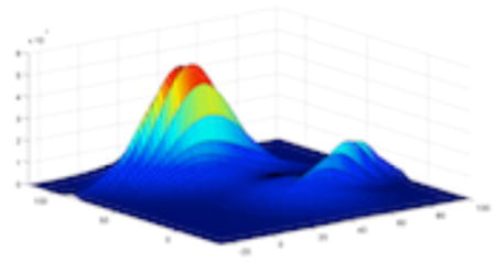
In the last part of our experimental results, we turn to the impact of the loss function on the CPXR(Log) algorithm. As mentioned earlier, (at least) three different loss functions can be used in CPXR(Log). Figure 4 shows how CPXR(Log)’s performance changes when different loss functions are used in the algorithm.

Figure 4.

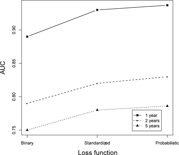
Impact of the loss function on CPXR(Log)’s performance

Clearly, the probabilistic loss function returns the most accurate models. In fact, the AUC obtained when the probabilistic loss function is used is 1% more than the AUC obtained when Pearson’s loss function, and 4.8% more than the AUC obtained when the binary loss function is used, on average for the 1 year, 3 year and 5 year HF survival models.

5. Conclusion

We used a new clinical prediction modeling algorithm, CPXR(Log) to build heart failure survival prediction models, for 1-, 2-, and 5-years after HF is diagnosed based on EHR data. The models built by CPXR(Log) achieved much higher accuracy than standard logistic regression, Random Forest, SVM, decision tree and AdaBoost, which implies that there are fairly complicated interactions between predictor and response variables for heart failure. We also included 24 co-morbidities into our models and showed that adding these new variables gives us both more insights and improved accuracy of our models. In general, CPXR(Log) can effectively build highly accurate prediction models on datasets with diverse predictor-response relationships, but the other classification algorithms cannot effectively handle the high dimensionality and complexity of EHR data in order to build accurate prediction models. This study indicates that the behavior of HF patients is highly heterogeneous and that different pat terns and local prediction models better suitable in predicting HF survival to properly handle the disease heterogeneity. We also proposed to use the probabilistic loss function in the CPXR(Log) algorithm, and the results showed the new loss function outperforms other loss function used in the previous studies.

Highlights.

• An approach called Contrast Pattern Aided Regression, CPXR(Log) with a new loss function is proposed.

• A series of heart failure survival risk models are developed using CPXR (Log) on an EHR dataset.

• The performance of CPXR(Log) models are compared with some of the state-of-the-art classification methods.

References

- 1.Heart disease and stroke prevention. http://www.cdc.gov/chronicdisease/resources/publications/AAG/dhdsp.htm. Accessed from July 2010.
- 2.Ouwerkerk W, Adriaan AV, Zwinderman AH. Factors influencing the predictive power of models for predicting mortality and/or heart failure hospitalization in patients with heart failure. JACC: Heart Failure. 2014;2.5:429–436. doi: 10.1016/j.jchf.2014.04.006. [DOI] [PubMed] [Google Scholar]
- 3.Gerber Y, Weston SA, Redfiled MM, Chamberlain AM, Manemann SM, Killian JM, Roger VL. A Contemporary Appraisal of the Heart Failure Epidemic in Olmsted County, Minnesota, 2000 to 2010. JAMA internal medicine. 2015 doi: 10.1001/jamainternmed.2015.0924. [DOI] [PMC free article] [PubMed] [Google Scholar]
- 4.Dunlay SM, Pereira NL, Kushwaha SS. Mayo Clinic Proceedings. Elsevier; 2014. Contemporary strategies in the diagnosis and management of heart failure; p. 89.5. [DOI] [PMC free article] [PubMed] [Google Scholar]
- 5.Levy WC, Mozaffarian D, Linker DT, Sutradhar SC, Anker SD, Cropp AB, Anand Maggioni A, Burton P, Sullivan MD, Pitt B, Poole-Wilson PA, Mann DL, Packer M. The Seattle Heart Failure Model prediction of survival in heart failure. Circulation. 2006;113.11:1424–1433. doi: 10.1161/CIRCULATIONAHA.105.584102. [DOI] [PubMed] [Google Scholar]
- 6.Brophy JM, Dagenais GR, McSherry F, Williford W, Yusuf S. A multivariate model for predicting mortality in patients with heart failure and systolic dysfunction. The American journal of medicine. 2004;16.5:300–304. doi: 10.1016/j.amjmed.2003.09.035. [DOI] [PubMed] [Google Scholar]
- 7.Koelling TM, Joseph S, Aaronson KD. Heart failure survival score continues to predict clinical outcomes in patients with heart failure receiving beta-blockers. J Heart Lung Transplant. 2004;23:1414–1422. doi: 10.1016/j.healun.2003.10.002. [DOI] [PubMed] [Google Scholar]
- 8.Gottlieb SS. Prognostic indicators: useful for clinical care. J Am Coll Cardiol. 2009;53(4):343–344. doi: 10.1016/j.jacc.2008.09.044. [DOI] [PubMed] [Google Scholar]
- 9.Califf RM, Pencina MJ. Predictive Models in Heart Failure: Who Cares? Circulation: Heart Failure. 6.5(2013):877–878. doi: 10.1161/CIRCHEARTFAILURE.113.000659. [DOI] [PubMed] [Google Scholar]
- 10.Letham B, Rudin C, McCormick TH, Madigan D. An Interpretable Stroke Prediction Model using Rules and Bayesian Analysis. AAAI (Late-Breaking Developments) 2013 [Google Scholar]
- 11.Dong G, Taslimitehrani V. Pattern-Aided Regression Modeling and Prediction Model Analysis. IEEE Transaction on Knowledge and Data Engineering. 2015;27.9:2452–2465. [Google Scholar]
- 12.https://www.whitehouse.gov/the-press-office/2015/01/30/fact-sheet-president-obama-s-precision-medicine-initiative
- 13.Taslimitehrani V, Dong G. A New CPXR Based Logistic Regression Method and Clinical Prognostic Modeling Results Using the Method on Traumatic Brain Injury. Proceedings of IEEE International Conference on BioInformatics and BioEngineering. 2014. 2014 Nov;:283–290. [Google Scholar]
- 14.Bagley SC, Halbert W, Golomb BA. Logistic regression in the medical literature: Standards for use and reporting, with particular attention to one medical domain. Journal of clinical epidemiology. 2001;54.10:979–985. doi: 10.1016/s0895-4356(01)00372-9. [DOI] [PubMed] [Google Scholar]
- 15.Kennedy RE, Livingston L, Riddick A, Marwitz JH, Kreutzer JS, Zasler ND. Evaluation of the Neurobehavioral Functioning Inventory as a depression screening tool after traumatic brain injury. The Journal of head trauma rehabilitation. 2005;20.6:512–526. doi: 10.1097/00001199-200511000-00004. [DOI] [PubMed] [Google Scholar]
- 16.Wei Y, Liu T, Valdez R, Gwinn M, Khoury MJ. Application of support vector machine modeling for prediction of common diseases: the case of diabetes and pre-diabetes. BMC Medical Informatics and Decision Making. 2010;1:16. doi: 10.1186/1472-6947-10-16. [DOI] [PMC free article] [PubMed] [Google Scholar]
- 17.Wu J, Roy J, Stewart WF. Prediction modeling using EHR data: challenges, strategies, and a comparison of machine learning approaches. Medical care. 2010;48.6:S106–S113. doi: 10.1097/MLR.0b013e3181de9e17. [DOI] [PubMed] [Google Scholar]
- 18.Zupan B, Demsar J, Kattan MW, Beck JR, Bratko I. Machine learning for survival analysis: a case study on recurrence of prostate cancer. Artif Intell Med. 2000;20(1):59–75. doi: 10.1016/s0933-3657(00)00053-1. [DOI] [PubMed] [Google Scholar]
- 19.Hertzong M, et al. Cluster Analysis of Symptom Occurrence to Identify Subgroups of Heart Failure Patients, A Pilot Study. Journal of Cardiovascular Nursing. 25.4(2010):273–283. doi: 10.1097/JCN.0b013e3181cfbb6c. [DOI] [PubMed] [Google Scholar]
- 20.Song Eun Kyeung, et al. Symptom clusters predict event-free survival in patients with heart failure. The Journal of cardiovascular nursing. 25.4(2010):284. doi: 10.1097/JCN.0b013e3181cfbcbb. [DOI] [PMC free article] [PubMed] [Google Scholar]
- 21.Alba CC, Agoritsas T, Jankowski M, Courvoisier D, Walter SD, Guyatt GH, Ross HJ. Risk Prediction Models for Mortality in Ambulatory Patients With Heart Failure A Systematic Review. Circulation: Heart Failure. 2013;6.5:881–889. doi: 10.1161/CIRCHEARTFAILURE.112.000043. [DOI] [PubMed] [Google Scholar]
- 22.Dai W, Brisimi TS, Adams WG, Mela T, Saligrama V, Paschalidis LC. Prediction of hospitalization due to heart diseases by supervised learning methods. International Journal of Medical Informatics. 2014;84.3:189–197. doi: 10.1016/j.ijmedinf.2014.10.002. [DOI] [PMC free article] [PubMed] [Google Scholar]
- 23.Panahiazar M, Taslimitehrani V, Pereira N, Pathak J. Using EHRs and Machine Learning for Heart Failure Survival Analysis. Studies in Health Technology and Informatics MedInfo. 2015;216:40–44. [PMC free article] [PubMed] [Google Scholar]
- 24.Ghanbarian B, Taslimitehrani V, Dong G, Pachepsky YA. Sample dimensions effect on prediction of soil water retention curve and saturated hydraulic conductivity. Journal of Hydrology. 2015;528:127–137. [Google Scholar]
- 25.U.S. Department of Health & Human Services. doi: 10.3109/15360288.2015.1037530. http://www.hhs.gov/ash/initiatives/mcc/ [DOI] [PubMed]
- 26.Fayyd U, Irani K. Multi-interval discretization of continuous-valued attributes for classification learning. Proc Int’l Joint Conf on Uncertainty in AI. 1993 [Google Scholar]
- 27.Dong G, Li J. Efficient mining of emerging patterns: Discovering trend and differences. Proc KDD. 1999:45–32. [Google Scholar]
- 28.R Core Team. R: A Language and Environment for Statistical Computing. R Foundation for Statistical Computing; Vienna, Austria: Version 2.14.1 (2011-12-22) [Google Scholar]
- 29.Su Yu-Sung, et al. Multiple imputation with diagnostics (mi) in R: Opening windows into the black box. Journal of Statistical Software. 2011;45:2. 1–31. [Google Scholar]
- 30.Memtsoudis Stavros G, et al. Risk factors for pulmonary embolism after hip and knee arthroplasty: a population-based study. International orthopaedics. 33.6(2009):1739–1745. doi: 10.1007/s00264-008-0659-z. [DOI] [PMC free article] [PubMed] [Google Scholar]