A convenient data structure for the nearest-neighbor problem is discussed.
Keywords: nearest-neighbor search, neartree data structure, post office problem
Abstract
Many problems in crystallography and other fields can be treated as nearest-neighbor problems. The neartree data structure provides a flexible way to organize and retrieve metric data. In some cases, it can provide near-optimal performance. NearTree is a software tool that constructs neartrees and provides a number of different query tools.
1. Introduction
Nearest-neighbor search (NNS) (also known as the post office problem; Knuth, 1998 ▸), has many uses. In crystallography, many geometric questions, e.g. inferring bonding from distances between atoms, can be resolved by NNS. It has other uses in pattern recognition (Zhang et al., 2006 ▸), computer graphics (Freeman et al., 2002 ▸), machine learning (Shaw & Jebara, 2009 ▸), tumor detection (Ballard & Sklansky, 1976 ▸) and other fields, including being a critical component of many data-mining algorithms. A considerable number of data structures have been developed to speed NNS. Examples are cubing (Levinthal, 1966 ▸), quadtrees (Samet, 1984 ▸), kd-trees (Bentley, 1975 ▸) and R-trees (Guttman, 1984 ▸). These differ from neartrees in that their internal structures are always aligned along coordinate axes. In neartrees, the orientations of the spatial divisions are derived from the relative positions of data points, independent of the coordinate system.
There are also closely related searches, such as k-nearest neighbors, range searches (Skiena, 1998 ▸) and farthest neighbor, as well as corresponding approximate searches for use when the exact answer is not required or is not feasible (Knuth, 1998 ▸; Muja & Lowe, 2014 ▸). The neartree data structure can be used in the implementation of each of these searches.
2. The nearest-neighbor problem
The nearest-neighbor search is well defined in any data space that satisfies the rules of a ‘metric space’. This means that there is a measure of distance, a ‘metric’, d(x, y), defined between all points x and y in the space, which is a non-negative real number for which a zero distance implies the points are equal, for which the distance is symmetric, i.e. d(x, y) = d(y, x), and for which the triangle inequality is satisfied, i.e. d(x, z) ≤ d(x, y) + d(y, z). Obviously, for a single probe datum, a simple linear search testing the distance to each data point will succeed. Searches can be complicated by issues such as the metric being discontinuous, the Hausdorff dimension of the data being high or the metric being time consuming to calculate. Direct application of the rules of a metric space may not work if multiple points are at zero distance from one another, e.g. two different atoms with partial occupancy at the same position, or two different structures with the same unit cell. These issues can all be addressed. If the search for the nearest datum is to be done for each of many probe data, then it is often advantageous to use an algorithm that reduces the number of distance calculations that must be performed. The linear search scales as O(n), where n is the number of points in the space. Optimal methods can scale by O[log(n)] for the average case (Kalantari & McDonald, 1983 ▸).
For those cases where the cost of distance evaluation is expensive, methods to reduce the number of evaluations are important, both in constructing the tree and in retrieving the sought datum. When multiple searches are needed, a linear search may be too expensive, even for testing a single probe at a time.
3. Searches related to the nearest-neighbor problem
Searches for nearest neighbors can be useful for exploring the vicinity of a probe. Farthest-neighbor search can be used to estimate the diameter of a data set (note this is only guaranteed to be the actual diameter in the one-dimensional case). Searches for all neighbors within a sphere or outside a sphere centered at the probe can be useful when the properties of a neighborhood are to be investigated (for instance, what atom types surround a particular atom in a protein). Searches for all the neighbors within an annulus centered at a probe can also be useful. Finally, the exact k-nearest-neighbor search has many uses. For instance, when a search might return a large number of results because of an unknown density of points, but a small sample would suffice, then the search could be limited to k. Surprisingly, rapid exact k-nearest-neighbor search has been found to be a somewhat difficult problem (Bernstein & Andrews, 2016 ▸).
There is also a considerable body of literature on the approximate k-nearest-neighbor search (see e.g. Knuth, 1998 ▸; Muja & Lowe, 2014 ▸). For some difficult problems, it is better to obtain at least an estimate of what the neighborhood is like. Approximate k-nearest-neighbor searches can be much faster than exact search, but obviously there are cases where an exact answer is preferred.
4. The neartree data structure
The ancestor of the neartree structure was described by Kalantari & McDonald (1983 ▸). Their structure is a double-linked tree, and retrieval is implemented using markers of where to resume searching when a branch has been bypassed. The concept was streamlined by Andrews (2001 ▸), where recursion replaces both the double linking and the inserted markers. Although the neartree structure is simpler to describe using recursion, implementation is more robust if one maintains an internal stack structure.
Neartrees can be used to store many kinds of data. The two requirements are that the data have a metric and that they obey the triangle inequality (that is, no one side of a triangle has a length that exceeds the sum of the lengths of the other two sides).
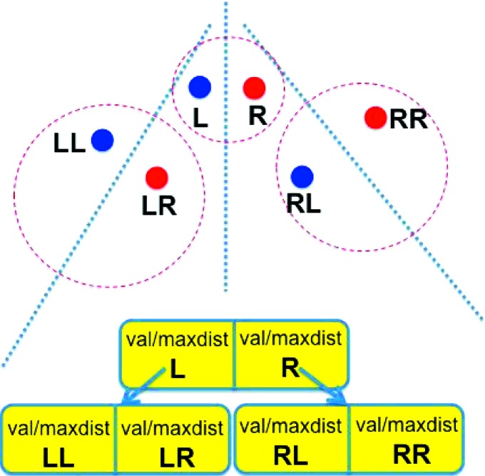
The neartree structure has a close resemblance to a binary tree. At each node, there is a right and a left point (see Fig. 1 ▸). In leaf nodes, there will be either one or two points. Each point stores a data object (or a reference to one) and the maximum distance from that data object to any data object in the subtree descending from the point. For the case of searching for the nearest (or farthest) neighbor of some probe point, that maximum distance frequently allows the search of some subtrees to be pruned (i.e. ignored). Kalantari & McDonald (1983 ▸) suggest that the use of more than two points in a node might be useful (resembling a B+ tree; Bayer & McCreight, 2002 ▸). Some experiments did not show consistent improvement in retrieval (Andrews, 1984 ▸).
Figure 1.
Example of a neartree containing six points. At the top of the figure we show the points in space. At the bottom of the figure we show the equivalent neartree. Each dashed circle in space represents one node, containing a pair of points, and each dotted line represents the partitioning of space for that node. The points in the root node are labeled ‘L’ and ‘R’. The points in the left node at the next level are labeled ‘LL’ and ‘LR’.
5. Limitations of neartrees in practice
The first limitation on neartrees is that the structure and the retrieval both require that the metric obey the triangle inequality. Small violations could lead to answers that are approximately correct, but, because incorrect pruning of the neartree search will occur, actual nearest neighbors could be missed. This problem is related to the requirement that, in a metric space, d(x, y) = 0 if and only if x = y. However, there is no requirement that the metric vary continuously. Discrete metrics, such as integers, work, and the objects stored in neartrees can be clusters of metric equivalent points. For example, in working with databases of unit cells, we store collision chains of structures with identical cells and just store a single representative of the collision chain in the tree proper.
Like any tree data structure, neartrees provide the best performance if they are relatively well balanced. Unfortunately, the standard methods for rebalancing a tree have a major drawback in neartrees. If a data point (or a subtree) is moved, many of the distances back to the root node will need to be recalculated. The only place that rebalancing does not incur a relatively large cost is at leaf nodes when a point is being added.
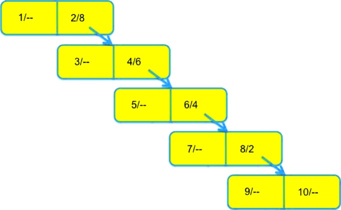
The loading of data into a neartree can influence the balancing of the tree. In a case where the data are sorted in some way before being added, unbalancing of the whole tree or multiple subtrees can result. As a particular unfortunate example, consider loading a sequence of integers into a neartree. When a datum is added to a filled node, it will be added to the subtree below the nearer of the two points. When the data are in sequence, then every filled node will have only a subtree on one side: a one-sided tree (see Fig. 2 ▸). Various schemes for randomizing the addition of data can mitigate this problem.
Figure 2.
An unbalanced neartree constructed by inserting, in order, the integers from 1 to 10.
Because the descending distances are stored in each node of a neartree, there are no simple methods either to delete points or to update the positions of points.
Bellman’s so-called ‘curse of dimensionality’ (Bellman, 1961 ▸) affects all schemes for improving NNS other than simple linear search. In high dimensions, it has been found that simpler NNS methods tend to become as slow as a linear search, because more and more points must be searched, asymptotically approaching all points.
6. Constructing a neartree
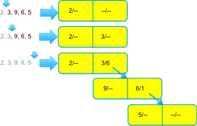
The algorithm will be described as a recursive algorithm. However, implementation by recursion to use a stack explicitly has the advantage of avoiding potential stack overflow, and it may lead to more efficient execution (see Fig. 3 ▸).
Figure 3.
An example of the growth of a neartree when inserting nodes in order as discussed in §6. The data consist of the integers 2, 3, 9, 6 and 5. The tree is empty when 2 and 3 are inserted, so 2 goes into the left side of the root node. 9 is closer to 3 than to 2, so it is inserted in the left side of a node pointed to from the right side of the root node, and the maximum distance on the right side of the root node is set to 6 = |9 − 3|. 6 is also closer to 3 than to 2, so it is inserted into the right side of the same child node. 5 is closer to 3 than to 2, so we follow the branch from the right side of the root node. We discover that 5 is closer to 6 than to 9, leading us to place 5 in a new child node pointed to from the right side of the previous child node and to set the maximum distance to 1 = |5 − 6|.
The procedure to add a new point at any node in a neartree is as follows:
(i) If the node does not exist, create an empty node.
(ii) If the node is empty, add the point as a new left point to the node (see the first line of Fig. 3 ▸).
(iii) Else if the node has only a left point, add the point as a new right point to the node.
(iv) Else if the node has both a right and a left point, determine which point contains the point that is closer to the new point (see the second line of Fig. 3 ▸).
(a) For that closer point, update the distance to the farthest point below in the neartree (see the final section of Fig. 3 ▸).
(b) If the distance from the point in the closer point to the new point is larger than the stored distance to the farthest point, update the distance (see the final section of Fig. 3 ▸).
(c) Otherwise, leave the maximum distance (below in the tree) unchanged.
(v) Add the point to the node that descends from that closer point, and return to step (i).
7. Searching a neartree for the nearest neighbor
As in adding a new point to a neartree, the algorithm is described using recursion. Implementation using other methods may be desirable.
To find the nearest point in a neartree to a probe point, start at the root node. There should be no empty nodes. Each node will contain one or two points.
(i) For the current node, determine which point is closer to the probe point. (If there is only one point in the node, it will be the left point.)
(a) For the closer point, calculate the distance from the probe to the point. If that is less than the shortest distance found so far, update the shortest known distance.
(b) Using the triangle inequality, determine whether the tree descending from the closer point could possibly contain a point closer than the current shortest distance. If the currently known shortest distance plus the farthest distance from the current point to any point below is less than the distance from the probe to the current point, then ignore any descending tree (see Fig. 4 ▸).
Figure 4.
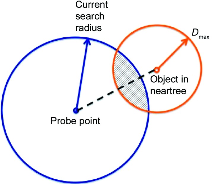
An example of a step in a search. Any possible objects that are closer than the current search radius lie only within the intersection of the circle around the probe point and the circle around the node object (with radius D max, the largest distance to any point below in the neartree). Only points in the crosshatched region can satisfy the triangle inequality for the particular objects. They satisfy the triangle inequality for the two circle centers.
(c) Otherwise, continue to search by taking the probe as the descending point [step (i)] (see Fig. 5 ▸).
Figure 5.
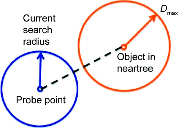
An example of a step in a search where the search cannot be completed. If the two circles do not intersect, then no object exists in the neartree that could form a triangle with the probe and the node object. In other words, D − d radius ≥ D max, where D is the distance between the probe point and the node object, and d radius is the current search radius. The inequality must be true if any further solutions are possible deeper in the tree.
(ii) Repeat the previous step [i.e. step (i)(a)] for the farther point (if any).
(iii) Output the shortest distance found from the probe to any point in the neartree.
8. Improving a neartree
One limitation of neartrees listed above is that inserting sorted data can lead to excessively unbalanced trees. Three schemes have been found to improve the balancing. The first (and simplest) is to delay insertion of new points into the tree until it is absolutely necessary to insert them (for instance, when a retrieval from the tree is requested). At that point in time, a random selection of points are added to the tree in random order. The best number of randomly selected points to use to initialize a balanced scaffold in the tree in this way is somewhat arbitrary; however, for n points, n 1/2 has been found to function relatively well.
The second scheme involves monitoring the depth of the tree during construction. When the currently constructed tree becomes too unbalanced, the random scheme (described above) can be invoked for the remaining uninserted points. This scheme can be particularly effective for cases such as the coordinates of a protein molecule, where the separate domains can cause a group of well sorted atoms to be processed sequentially.
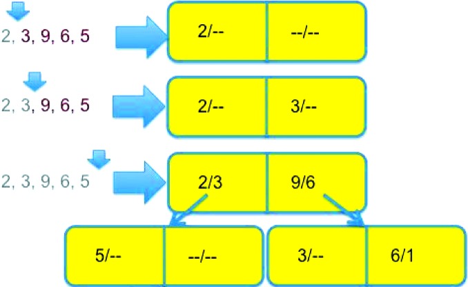
The third scheme (the ‘flip’) improves the depth of the tree by improving the separation between pairs of points in nodes. In the course of inserting a new point P in the tree, when a leaf node with left point L and right point R is encountered, the distances d(P, L) and d(P, R) have to be computed in order to decide whether to insert P in the subtree that descends from L or in the one that descends from R. If d(P, L) is larger than d(L, R), replace L with P in the node and insert P in the subtree that now descends from P. If d(P, R) is larger than d(L, R), replace R with P in the node and insert R in the subtree that now descends from P. See Fig. 6 ▸ for an example of the process.
Figure 6.
An example of the growth of a neartree when inserting nodes in order, with the ‘flip’ logic discussed in §8 enabled. We use the same data as in Fig. 3 ▸, but the tree grows differently because we are allowed to flip already-inserted data further down into the tree to achieve a better balance. The first two data points, 2 and 3, are first inserted as before, but when we get to 9, as before we see that 9 is closer to 3 than it is to 2, but also further from 2 than 3 is, so we replace 3 in the root node with 9 and insert 3 on the left side of a node pointed to by the right side of the root node, where 9 would have gone before. Note that the maximum distance on the right side of the root node is still 6 = |3 − 9|. The inserted 6 goes as before, because 6 is closer to 9 than it is to 2, but 5 now goes to the left branch of the root node, because 5 is closer to 2 than it is to 9.
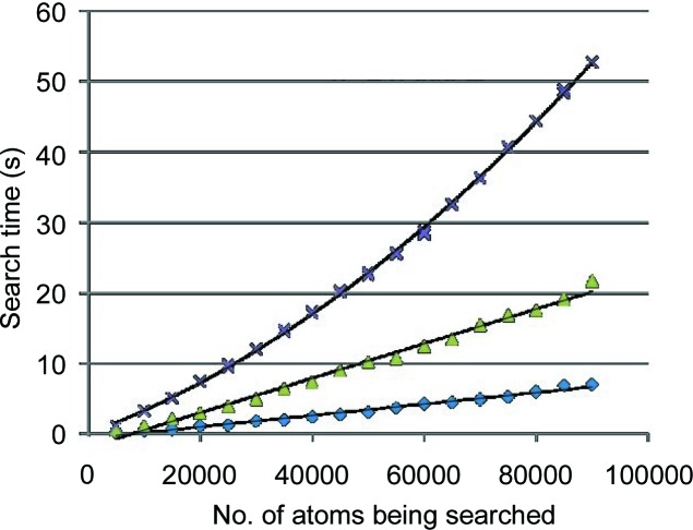
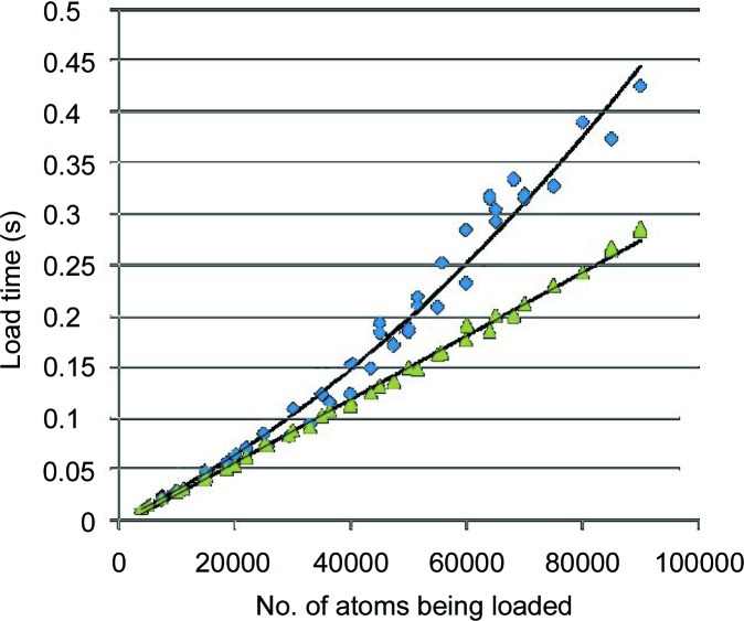
Each of these schemes contributes to shallower trees, which result in a shorter average time to retrieve nearest neighbors (see Fig. 7 ▸). However, the third scheme does result in somewhat slower tree builds (see Fig. 8 ▸). For a tree of fewer than 100 000 nodes, the cost is justified if there will be at least two searches for each tree build. For larger trees with several million nodes and more and a small number of searches per build, the second scheme is sometimes preferable.
Figure 7.
Using NearTree to identify nearest neighbors for each atom in partial sets of coordinates from PDB entry 1jj2 (Klein et al., 2001 ▸). For each group, every atom is searched for its nearest neighbor. The expected order is O[nlog(n)]. The top curve is for all atoms in a group inserted into the tree in sequential order. The middle curve is for initially inserting n 1/2 randomly selected points. The bottom curve uses more insertion randomization based on measured differences in subtree depths, as well as applying the ‘flip’ logic discussed in §8.
Figure 8.
Using NearTree to identify nearest neighbors for each atom in partial sets of coordinates from PDB entry 1jj2 (Klein et al., 2001 ▸). For each group, every atom is searched for its nearest neighbor. The expected order is O[nlog(n)]. The top curve is for all atoms in a group inserted into the tree in sequential order. The bottom curve uses more insertion randomization based on randomly selected points and on measured differences in subtree depths, as well as applying the ‘flip’ logic discussed in §8.
9. NearTree, a package and interface for searching
NearTree is a collection of functions for constructing and searching a neartree data structure. NearTree has been used for a wide range of applications, including as the engine for inferring the connectivity of molecular structures for which only three-dimensional atomic coordinates are known (replacing the traditional use of Levinthal cubing in RasMol; Bernstein, 2000 ▸), and in ocean color analysis (Klein et al., 2001 ▸), sonic boom prediction (Park & Darmofal, 2010 ▸), elastoplastics simulations (Wicke et al., 2010 ▸), transportation systems (Homerick, 2010 ▸), estimation of molecular surfaces (Bernstein & Craig, 2010 ▸), lattice identification (Andrews & Bernstein, 2014 ▸) and searching the Protein Data Bank (PDB) for entries matching experimental cells (McGill et al., 2014 ▸).
10. Conclusion
The neartree structure enables simple methods for probing the environments of points in a geometric space. Many important problems in engineering and science can be addressed as problems in geometry. Neartrees provide a technique for creating databases that can be queried using user-selected precision, rather than requiring fixed scalar key values. The NearTree implementation has been found to outperform other software for the NNS (Bernstein & Craig, 2010 ▸). The NearTree package of open source code provides code to construct neartrees and to retrieve results using several search techniques: nearest point, all nearest within a zone and all within a zone around the probe. The same are provided for farthest points and for only some specified number of results.
11. Availability of NearTree
The latest version of the source code of NearTree is maintained at http://sf.net/projects/neartree.
Acknowledgments
The authors express their thanks to Frances C. Bernstein for helpful suggestions and comments. This work was supported in part by US NIGMS grant No. GM078077.
References
- Andrews, L. C. (1984). Personal communication.
- Andrews, L. C. (2001). C/C++ Users J. 19, 40–49. http://www.drdobbs.com/cpp/a-template-for-the-nearest-neighbor-prob/184401449.
- Andrews, L. C. & Bernstein, H. J. (2014). J. Appl. Cryst. 47, 346–359. [DOI] [PMC free article] [PubMed]
- Ballard, D. H. & Sklansky, J. (1976). IEEE Trans. Comput. 100, 503–513.
- Bayer, R. & McCreight, E. (2002). Organization and Maintenance of Large Ordered Indexes. Berlin, Heidelberg: Springer.
- Bellman, R. (1961). Adaptive Control Processes: A Guided Tour. Princeton University Press.
- Bentley, J. L. (1975). Commun. ACM, 18, 509–517.
- Bernstein, H. J. (2000). Trends Biochem. Sci. 25, 453–455. [DOI] [PubMed]
- Bernstein, H. J. & Andrews, L. C. (2016). J. Appl. Cryst. 49. Submitted. [DOI] [PMC free article] [PubMed]
- Bernstein, H. J. & Craig, P. A. (2010). J. Appl. Cryst. 43, 356–361. [DOI] [PMC free article] [PubMed]
- Freeman, W. T., Jones, T. R. & Pasztor, E. C. (2002). IEEE Comput. Graph. 22(2), 56–65.
- Guttman, A. (1984). SIGMOD ’84. Proceedings of the 1984 ACM SIGMOD International Conference on Management of Data, Vol. 14, Part 2, pp. 14–57, 10.1145/602259.602266. New York ACM.
- Homerick, D. J. (2010). MSc thesis in Computer Science, University of California Santa Cruz, USA.
- Kalantari, I. & McDonald, G. (1983). IEEE Trans. Software Eng. 36, 631–634.
- Klein, D. J., Schmeing, T. M., Moore, P. B. & Steitz, T. A. (2001). EMBO J. 20, 4214–4221. [DOI] [PMC free article] [PubMed]
- Knuth, D. E. (1998). The Art of Computer Programming, Vol. 3, Searching and Sorting, 2nd ed., ch. 6.5, pp. 559–582. Reading: Addison-Wesley.
- Levinthal, C. (1966). Sci. Am. 214(6), 42–52. [DOI] [PubMed]
- McGill, K. J., Asadi, M., Karakasheva, M. T., Andrews, L. C. & Bernstein, H. J. (2014). J. Appl. Cryst. 47, 360–364. [DOI] [PMC free article] [PubMed]
- Muja, M. & Lowe, D. G. (2014). IEEE Trans. Pattern Anal. 36, 2227–2239. [DOI] [PubMed]
- Park, M. A. & Darmofal, D. L. (2010). AIAA J. 48(9), 1–40.
- Samet, H. (1984). ACM Comput. Surveys, 16, 187–260.
- Shaw, B. & Jebara, T. (2009). Proceedings of the 26th Annual International Conference on Machine Learning, pp. 937–944. New York: ACM.
- Skiena, S. S. (1998). The Algorithm Design Manual: Text. Heidelberg: Springer Science and Business Media.
- Wicke, M., Ritchie, D., Klingner, B. M., Burke, S., Shewchuk, J. R. & O’Brien, J. F. (2010). ACM Trans. Graph. 29(4), 49:1–49:11.
- Zhang, H., Berg, A. C., Maire, M. & Malik, J. (2006). Proceedings of the IEEE Computer Society Conference on Computer Vision and Pattern Recognition, Vol. 2, pp. 2126–2136. New York: IEEE.


