

Abstract
Tsunamis generated by landslides and volcanic island collapses account for some of the most catastrophic events recorded, yet critically important field data related to the landslide motion and tsunami evolution remain lacking. Landslide-generated tsunami source and propagation scenarios are physically modelled in a three-dimensional tsunami wave basin. A unique pneumatic landslide tsunami generator was deployed to simulate landslides with varying geometry and kinematics. The landslides were generated on a planar hill slope and divergent convex conical hill slope to study lateral hill slope effects on the wave characteristics. The leading wave crest amplitude generated on a planar hill slope is larger on average than the leading wave crest generated on a convex conical hill slope, whereas the leading wave trough and second wave crest amplitudes are smaller. Between 1% and 24% of the landslide kinetic energy is transferred into the wave train. Cobble landslides transfer on average 43% more kinetic energy into the wave train than corresponding gravel landslides. Predictive equations for the offshore propagating wave amplitudes, periods, celerities and lengths generated by landslides on planar and divergent convex conical hill slopes are derived, which allow an initial rapid tsunami hazard assessment.
Keywords: landslide, tsunami, physical model, wave generation
1. Introduction
Tsunamis are generated by impulsively displacing a volume of water and can be generated by submarine earthquakes and landslides, volcanic eruptions and asteroid impacts [1]. Landslide-generated tsunamis can occur in confined bays, lakes, reservoirs, at islands or at continental shelf breaks, and are particularly hazardous in the near-field region, producing locally extremely large amplitude waves and run-up [2]. Landslide-generated tsunamis can be classified as subaerial, partially submerged or submarine, depending on the initial landslide position. Major subaerial and partially submerged landslide impact-generated tsunamis occurred at Knight Inlet in British Columbia, Canada (1500s) [3], Tafjord (1934) and Lake Loen (1936) in Norway [4,5], Lituya Bay, AK, USA, in 1958 [6–9], Vajont Dam in Italy in 1963 [10,11], Yanahuin Lake, Peru, in 1971 [12], Fatu Hiva (Marquesas Islands; French Polynesia) in 1999 [13], Aisén Fjord, Chile, in 2007 [14,15], Chehalis Lake in British Columbia, Canada, in 2007 [16–18] and in Haiti in 2010 [19]. Tsunamis generated by submarine landslides were associated with the ancient Storegga slides [20,21], and were observed in Puerto Rico in 1918 [22], Grand Banks, Newfoundland, in 1929 [23] and Papua New Guinea in 1998 [24,25]. Tsunamis generated by volcanic activity associated with eruptions or gravitational flank collapses have been recorded at Mount Unzen, Japan, in 1792 [26], Ritter Island, New Guinea, in 1881 [27], Krakatau, Indonesia, in 1883 [28] and Stromboli, Italy, in 2002 [29,30].
Field data from these events are limited to the landslide scarp, run-up trimline, far-field tide gauge recordings and the submarine deposit, where mapped. Physical models are used to study the wave generation, propagation and run-up of impulsively generated waves. The subaerial landslide tsunami generation process is a transient multi-phase flow involving unsteady interaction between the landslide material, water and air. Historically, physical modelling of landslide-generated tsunami focused on two-dimensional models with a solid block sliding down an inclined slope [31–46] or with granular landslides [9,47–54]. Three-dimensional models using a solid block slide on a plane hill slope were studied by Liu et al. [55], Lynett & Liu [56], Panizzo et al. [57], Enet & Grilli [58,59] and Grilli & Watts [35], and a solid block slide on a conical hill slope was performed by Di Risio et al. [60] and Romano et al. [61]. Direct comparisons of two-dimensional and three-dimensional block models on planar hill slopes were studied by Heller & Spinneken [62] and Heller et al. [63]. Lindstrøm et al. [64] physically modelled the potential Åknes landslide with a block slide in a scaled model of Storfjorden in Norway. Tsunami wave evolution around a conical island originating from offshore was physically modelled by Yeh et al. [65], Briggs et al. [66] and Liu et al. [67]. Granular landslides were studied in three-dimensional model basins with an inclined channel by Huber [51] and a planar hill slope by Mohammed & Fritz [68,69]. This study extends the physical modelling of three-dimensional tsunami generation by including gravel and cobble landslide material in various topographic scenarios. This study analyses the offshore propagating waves. Owing to manuscript length requirements and the exhaustive run-up analysis performed, the run-up analysis will be included in a separate manuscript.
2. Experimental set-up
Physical model experiments based on real-world events using Froude similarity were conducted at the George E. Brown Network of Earthquake Engineering and Simulation (NEES) tsunami wave basin (TWB) at Oregon State University in Corvallis, OR, USA. The concrete TWB is 48.8 m long, 26.5 m wide and 2.1 m deep. The offshore propagating wave is studied in two topographic and bathymetric scenarios, basin-wide propagation and run-up scenario, and conical island scenario, shown in figure 1a,b, respectively. The effects of the lateral hill slope are studied by comparing the offshore propagating wave characteristics between the two scenarios. A total of 159 experimental trials were conducted in these two configurations, 39 of which were repeated trials. Landslides are modelled using a unique landslide tsunami generator (LTG) shown in figure 1c and described by Mohammed & Fritz [68], which can simulate landslides with varying geometry and kinematics. The LTG consists of a sliding box filled with 0.756 or 0.378 m3 of landslide material which is accelerated by means of four pneumatic pistons down a 27.1° slope. This hill slope, α, is selected to match the natural angle of repose of natural sediments and hill slopes. Near peak box velocity, the landslide material exits the slide box and continues to accelerate solely by gravity towards the water surface. Landslides were deployed into water depths, h, of 0.3, 0.6, 0.9 and 1.2 m. Two different landslide materials were used to study the effects of the landslide granulometry on the wave characteristics. Naturally rounded river gravel was used in both scenarios with a grain size gradation of 95% passing the 19.1 mm sieve, 5% passing the 12.7 mm sieve and median grain size diameter (d50) of 13.7 mm. In the conical island scenario, naturally rounded river cobbles were tested with a grain size diameter larger than the 19.1 mm, and some cobbles were larger than 100 mm in all dimensions. The landslide materials can be seen in figure 1d,e. Both landslide materials had a slide grain density ρg=2.6 t m−3, bulk slide density ρs=1.76 t m−3, porosity n=0.31, internal friction angle ϕ′=41° and basal friction angle on steel δ=23°. The two landslide volumes tested correspond to masses of 1350 and 675 kg. The granular landslide material used in the present model is similar to past granular landslide models that match the bulk slide characteristics of subaerial rock landslides [48,68,70]. The results from the present model may not appropriately scale to cohesive materials, such as clays, or fine particle sediments, such as sands and silts [71–73].
Figure 1.

Wave gauge array used in the Network for Earthquake Engineering and Simulation (NEES) tsunami wave basin at the O.H. Hinsdale Wave Research Laboratory at Oregon State University, Corvallis, OR, with water depth of h= 0.3 m forthe (a) basin-wide propagation and run-up scenario and (b) conical island scenario. (c) Pneumatic landslide tsunami generator (LTG) in the retracted position after launching landslide material; naturally rounded (d) river gravel and (e) river cobble landslide materials.
The investigated parameters that govern tsunami generation by granular landslides are the water depth, h, slide impact front velocity, vs, slide thickness, s, slide width, b, slide volume, V s, and shoreline radius, rc. The corresponding non-dimensional parameters are the landslide Froude number, F, relative slide thickness, S, relative slide width, B, relative landslide volume, V , and relative shoreline radius, Rc. The landslide Froude number is defined as . The landslide Froude number is the ratio of the slide impact front velocity and the linear shallow water depth wave celerity, . Because the landslide Froude number, F, is proportional to h−0.5, the slide Froude number is more sensitive to the landslide impact velocity than the water depth. The landslide Froude number is tested in the range 1.05≤F≤3.85. Typical real-world subaerial landslide-generated tsunamis are in the range of 1<F<4 and submarine landslide-generated tsunamis are typically in the range F<1. The subaerial landslide-generated tsunami in Lituya Bay, AK, USA, in 1958 produced the largest recorded wave run-up of 524 m with a landslide Froude number of F=3.2, in a water depth of h=122 m at the impact site and landslide impact velocity of vs=110 m s−1 [6].
The relative slide thickness and width are measured at impact and are, respectively, defined as S=s/h and B=b/h. The relative slide thickness, S, is determined by the water depth and the local landslide thickness, s, which is dependent on the landslide motion and downslope sliding distance. The relative thickness is tested in the range of 0.08≤S≤0.46. The relative landslide width, B, is determined by the water depth and the local slide width, b, which is dependent on the landslide motion, downslope sliding distance and the lateral hill slope curvature. The convex conical hill slope of the conical island scenario produced larger landslide widths at impact than the planar hill slope. The relative landslide width at impact on the planar hill slope is in the range 1≤B≤7. Minor differences are observed in the slide width between the gravel and cobble landslides on the convex conical hill slope. The relative slide width on the convex conical hill slope is in the range 1.4≤B≤11.7 for the gravel landslide and 1.4≤B≤11.2 for the cobble landslide.
The relative landslide volume is defined as V =V s/h3. The relative landslide volume is dependent on the dimensional landslide volume and the water depth. The relative landslide volume is tested in the range 0.2≤V ≤28. The landslide length scale is given as Ls=V s/(sb), thus the relative slide length is defined as L=Ls/h, and is tested in the range 0.7≤L≤34. The relative shoreline radius is only applicable to the conical island scenario and is defined as Rc=rc/h, where rc is the dimensional shoreline radius. The relative shoreline radius is an important parameter for describing the curvature of the shoreline and is tested in the range 2.2≤Rc≤14.7.
State-of-the-art instrumentation is deployed in the wave basin to measure the characteristics of the landslide motion and the wave properties of the tsunami-generated waves. Water surface elevations are recorded by an array of resistance wave gauges. The landslide evolution is measured from above and underwater camera recordings. The landslide deposit is measured on the basin floor with a multiple transducer acoustic array. Landslide surface velocities are determined with a stereo particle image velocimetry system. Wave run-up is recorded with resistance wave gauges along the slope and validated with video image processing.
The offshore waves are investigated in the basin-wide propagation and the conical island scenarios. In the basin-wide propagation and run-up scenario, 18 offshore wave gauges are analysed between the two planar hill slopes. The two wave gauges in proximity to the opposing hill slope are omitted from this offshore wave propagation analysis owing to interfering wave reflections. The analysed offshore gauges are spaced in a radial and angular array within the ranges of 3<r/h<50 and 0°≤θ≤75°. Similarly, in the conical island scenario, 21 offshore wave gauges are analysed in a radial and angular array within the ranges of 3<r/h<50 and 0°≤θ≤86°. The gauge locations in the basin-wide propagation and the conical island scenarios are shown in figure 1a,b.
The origin of the cylindrical coordinate system is defined as the intersection of the longitudinal landslide motion centre and the waterline on the hill slope. The gauges remained constant, but the relative position of the wave gauges, r/h, along given wave angle, θ, varied dependent on the water depth. In both scenarios, 10 wave gauges are cantilevered from the instrumentation bridge, whereas the remaining wave gauges are mounted in the basin. The instrumentation bridge is placed close enough to the wave generation source to measure the water surface elevation in the near-field region while avoiding landslide run-out. The gauge locations are strategically placed to directly compare the waves between the two scenarios and investigate the influence of the lateral hill slope on the offshore propagating wave.
3. Landslide source and tsunami generation
The landslide material is initially in the slide box and is accelerated by four pneumatic pistons. Near peak box velocity, the landslide smoothly transitions out of the slide box to the hill slope and continues to accelerate by gravitational force towards the water while decreasing the slide thickness and increasing the slide width [74]. The coordinate system for the landslide travel distance down the hill slope is noted as xs, and the origin is set at the initial slide box front. The landslide front velocity is measured with side view and high-resolution (2.8 mm per pixel in the object plane) overhead cameras. The evolutions of the landslide front velocity with distance down the hill slope for gravel landslides on planar and conical hill slopes, along with cobble landslides on a conical hill slope, are shown in figure 2a,b. Similarly, the landslide thickness and width are measured with overhead and side view cameras. The landslide velocity, thickness and width at impact determine the landslide mass, momentum and energy fluxes. The landslide evolution shown in figure 2 is normalized by the initial slide thickness, so, rather than the water depth, h, to clearly show the landslide evolution at all water depths.
Figure 2.

Subaerial slide evolution: dimensionless landslide front velocity vs/(gso)1/2 as a function of propagation distance down the hill slope after the landslide exits the slide box with a slide volume of (a) and (b) ; dimensionless landslide maximum thickness, sm/so, as a function of propagation distance down the hill slope with a slide volume of (c) and (d) ; dimensionless landslide width, bm/so, with a slide volume of (e) and (f) , where the gravel landslide on the planar hill slope is black, on the conical hill slope is red and the cobble landslide on the conical hill slope is blue. The initial slide box front is xs=0. The slide launch velocities with slide volume are vs/(gso)1/2=1.3 (dotted), vs/(gso)1/2=1.6 (dashed-dot), vs/(gso)1/2=1.8 (dashed) and vs/(gso)1/2=2.2 (solid), and slide volume are vs/(gso)1/2=1.3 (dotted), vs/(gso)1/2=1.6 (dashed-dot), vs/(gso)1/2=1.9 (dashed) and vs/(gso)1/2=2.3 (solid). The water impact locations for the tested depths of h=0.3, 0.6, 0.9 and 1.2 m correspond to xs/so=13.5, 11.3, 9.1 and 7.0, respectively.
Variability in the wave measurements can be attributed to uncertainties in the landslide impact parameters. Uncertainty in the landslide measurements can be estimated by the absolute value of error in the camera image measurements and is based on the image calibration and scaling. The maximum relative error in the dimensionless landslide parameters cannot exceed the sum of the relative error from the dimensional components [75]. The maximum uncertainties for the landslide front velocity, thickness and width are estimated as 3%, 2.7% and 3%, respectively. The uncertainty in the measurement of the water depth is estimated as 1.7%. Therefore, the maximum uncertainties for F, S, B and V are 3.8%, 4.4%, 4.7% and 5.0%. Repeated landslide measurements found the differences in non-dimensional parameters to be less than 3% [76].
The offshore propagating wave characteristics are dependent on the landslide impact characteristics [48,68]. The landslide tsunami generation process is shown in figure 3 with a gravel landslide on a divergent convex conical hill slope. The landslide impacts the water and transfers kinetic energy to the water body. This displaces the water in the impact region primarily in the landslide motion direction, but also laterally around the landslide front. This displacement produces a radial wave crest that propagates away from the impact site. The engulfing landslide creates an impact crater by drawing down the water surface in the impact region, which becomes the leading wave trough. Crater collapse and gravitational restoring forces drive the vertical fluid uprush and onshore run-up, evolving into the second wave crest. As the trailing wave crest propagates away from the impact site, several oscillating water surface depressions and elevations occur resulting in the subsequent waves. Nonlinear transition-type wave profiles generated by gravel landslides on planar and conical hill slopes and cobble landslides on conical hill slopes are shown in figure 4. The size of the impact crater generated on both planar and convex conical hill slopes varies with the landslide impact velocity, slide thickness and slide width. This is due to the mass and momentum flux being primarily dependent on these impact parameters.
Figure 3.
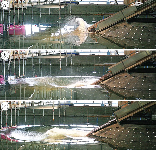
Wave generation: (a) gravel landslide impacts the water body and the initial water displacement becomes the radially propagating leading wave crest, (b) the landslide creates an impact crater in the water surface which becomes the leading wave trough and (c) the crater collapses producing the second wave crest. (Online version in colour.)
Figure 4.

Propagation of landslide-generated waves with slide parameters F=3.8, S=0.46, V =14, h=0.3 m (corresponding to slide evolution measurements in figure 2 of vs/(gso)1/2=2.2 and ) measured at (a) θ=0°, r/h=11.6, (b) θ=30°, r/h=13.4 and (c) θ=60°, r/h=15.2, and with slide parameters F=1.1, S=0.18, V =0.44, h=1.2 m (corresponding to slide evolution measurements of vs/(gso)1/2=1.6 and ) measured along θ=0° at (d) r/h=4.4, (e) r/h=7.8 and (f) r/h=11.9.
4. Wave amplitude
(a). Wave amplitude attenuation and prediction
Tsunami wave crest and trough amplitudes are critical hazards with each posing its own danger. In the near-field region, impulsively generated waves are commonly in the nonlinear regime, deviating from the equipartition characteristic of linear waves. Wave crest and trough amplitudes are analysed individually because of the varying amplitudes and celerities of each component. Predictive equations for individual wave crest and trough amplitudes often note inversely proportional wave generation parameters, making a single maximum wave amplitude predictive equation practically challenging.
Mohammed & Fritz [68,69] produced predictive equations using multi-variable regression analysis for the leading wave crest and trough amplitudes introducing the form a/h=kaf(r/h,θ), where the wave amplitude, a, is non-dimensionalized by water depth, h, whereas ka represents a wave generation function coupled with an amplitude decay function involving the radial distance from the source, r, and the wave ray angle, θ. Empirical equations for the individual wave amplitudes are given by Mohammed & Fritz [68] and applied to the current dataset as
| 4.1 |
| 4.2 |
| 4.3 |
for the first wave crest, ac1, first wave trough, at1, and second wave crest, ac2. The second wave crest decays more rapidly in the angular direction than the leading wave owing to the differing wave generation mechanisms [68]. The radial propagation decay function, n, describes the amplitude decay owing to three-dimensional energy spreading, frequency dispersion and nonlinear effects. Effects of the higher-order nonlinear amplitude dispersion were observed in the propagating wave celerity. The wave generation is described as a function of the landslide impact and hill slope characteristics, ka=g(F,S,B,V,L,α,Rc). The planar hill slope equations are expanded for applicability to convex conical hill slopes by deriving coefficients for the amplitude generation and propagation decay functions. The wave amplitude generation, ka, and radial propagation decay, na, functions are given as
| 4.4 |
| 4.5 |
| 4.6 |
| 4.7 |
| 4.8 |
| 4.9 |
where C is the conical hill slope coefficient which is equal to 1 for planar hill slopes. The conical hill slope coefficients are given as
| 4.10 |
| 4.11 |
| 4.12 |
| 4.13 |
| 4.14 |
| 4.15 |
where all the conical hill slope coefficients are functions of the dimensionless shoreline radius, Rc, which smoothly transitions the coefficients to 1 for large radiuses approaching planar hill slopes. The wave amplitude conical coefficients, C, were derived using a nonlinear least-squares solving technique with a fixed form and ranged in this study from 0.4 to 2.1. The leading wave crest amplitude in this study results in an r2 correlation coefficient of 0.94 with a gravel landslide on a planar hill slope and 0.93 with gravel and cobble landslides on a convex conical hill slope. The predictive equation for the leading wave trough on planar and convex conical hill slopes result in an r2 correlation coefficient of 0.94 and 0.95, respectively. The predictive equations for the second wave crest on the planar and convex conical hill slopes produce an r2 correlation coefficient of 0.87 and 0.88, respectively. The measured versus predicted leading wave crest and trough amplitudes are shown in figure 5a,b.
Figure 5.

Comparison of the measured and predicted (a) leading wave crest amplitude, ac1/h, and (b) leading wave trough amplitude, at1/h, where the gravel slide material on a planar hill slope is denoted with blue symbols, on a convex conical hill slope with cyan symbols, and the cobble landslide material on a conical hill slope with red symbols. The 30% and 50% error thresholds are shown with dashed lines. Lateral hill slope effects: comparison of the wave amplitudes generated on planar and convex conical hill slopes for the (c) leading wave crest and (d) leading wave trough. Granulometry effects: comparison of the wave amplitude between gravel and cobble landslides for the (e) leading wave crest and (f) leading wave trough.
The expanded predictive equation for the leading wave crest on a planar hill slope matches the equation by Mohammed & Fritz [68]. Measurements of the second crest's amplitude at the water depth h=0.3 m in this study extend the range of parameters incorporated in the second wave crest amplitude predictive equation compared with Mohammed & Fritz [68]. The first wave trough and second wave crest amplitude data from the physical model described in Mohammed & Fritz [68] were combined with amplitude data from the planar hill slope in this study to produce the respective expanded predictive equations.
The leading wave crest amplitude is a function of the landslide Froude number, F, and relative slide thickness, S, and the amplitude decay is inversely proportional to the relative slide width, B. The strong dependency of the wave amplitude on the landslide Froude number and the slide thickness was shown in two-dimensional granular experiments by Fritz et al. [48]. Increasing the landslide Froude number produces a larger initial displacement of water, resulting in a larger leading wave crest. Decreasing the slide width leads to a generation mechanism closer to a point source with increasing radial decay. The leading wave trough is a function of the landslide Froude number, F, relative slide thickness, S, and relative slide length, L. The leading wave trough is generated by the drawdown produced when the landslide impacts the water surface and is dependent on the landslide velocity and length scales, as noted in the equation. The second wave crest is generated by the collapse of the impact crater and is a function of the landslide Froude number, F, thickness, S, width, B, and length, L.
(b). Lateral hill slope effects
The lateral hill slope effects on the wave amplitude are compared between the planar and convex conical hill slopes. The ratio of wave amplitudes (aplan/acon) generated by a gravel landslide on planar (aplan) and convex conical (acon) hill slopes for the first wave crest, first wave trough and second wave crest are in the ranges 0.85≤ac1 plan/ac1 con≤1.17, 0.40≤at1 plan/at1 con≤1.30 and 0.42≤ac2 plan/ac2 con≤1.64. The mean values for the lateral hill slope ratios for the first wave crest, first wave trough and second wave crest are 1.02, 0.88 and 0.86, respectively. The measured wave amplitudes generated by a gravel landslide on planar and convex conical hill slopes are shown in figure 5c,d. The corresponding leading wave crest amplitude is on average larger when generated on the planar hill slope than on the convex conical hill slope. In contrast, the corresponding leading wave trough and second wave crest are on average smaller when generated on the planar hill slope than on the convex conical hill slope. The lateral hill slope plays a more significant role in the impact crater formation evolving into the leading wave trough and crater collapse with subsequent uprush resulting in the second wave crest. The increased amplitude of the leading wave trough and second wave crest on the convex conical hill slope may be attributed to the curvature of the island shoreline being closer to normal with the wave rays of the offshore propagating radial waves than the planar hill slope [76]. Increased wave amplitude normal to the hill slope has been observed in previous planar hill slope studies [57,62,68,76,77].
(c). Landslide granulometry effects
The effects of the landslide granulometry are analysed by comparing the corresponding wave amplitudes generated by gravel and cobble landslides on the convex conical hill slope. The ratios of the wave amplitudes generated by cobble (acob) and gravel (agrav) landslides for the first wave crest, first wave trough and second wave crest are in the ranges 1.08≤ac1 cob/ac1 grav≤1.51, 1.08≤at1 cob/at1 grav≤1.46 and 0.82≤ac2 cob/ac2 grav≤1.28. The mean values for the granulometry ratios are 1.25, 1.20 and 1.11 for the first wave crest, first wave trough and second wave crest, respectively. On average, the cobble landslide produced mostly larger wave amplitudes than the corresponding gravel landslide with the differences being most pronounced for the first wave crest and trough. The wave amplitudes generated by cobble and gravel landslides on the convex conical hill slope are shown in figure 5e,f.
The larger wave amplitude created by the cobble than by the gravel landslide may be due to a more efficient energy transfer from the landslide to the wave. It is observed that the corresponding cobble landslide width remains narrower than the gravel landslide on the convex conical hill slope. Although the maximum thickness in the centre of the landslide is equivalent between the landslide materials, the average thickness across the cobble landslide width decays less rapidly than that of the gravel landslide. The larger cobbles also have more inertia to displace water than smaller gravel granulates. This is visualized by the hummocky features in the deposits with larger cobbles producing larger run-out than smaller material.
(d). Comparison with previous studies
Panizzo et al. [57] physically modelled landslide-generated tsunamis in a three-dimensional basin with vertical walls using a sliding block on a rectangular trolley ramp to reach F≤2.22. Similar to the two-dimensional approach by Watts [34], the relative time of underwater motion was determined to be an important factor which is given as
| 4.16 |
The predicted first wave height by Panizzo et al. [57] is given by
| 4.17 |
where is the dimensionless front cross-section given as A*w=(bs)/h2. The mechanical stoppers used in the Panizzo et al. [57] model at the toe of the ramp abruptly cropped the underwater slide run-out and significantly reduced the duration of slide motion compared with the granular landslide run-out. This results in an underprediction by a factor of 2 when applying equation (4.17) to this study. Doubling the predicted values from equation (4.17) produces an r2 correlation coefficient of 0.94 with the leading wave height generated with a gravel landslide on a planar hill slope, matching the results discussed in Mohammed & Fritz [68].
Huber [51] conducted three-dimensional physical experiments on landslide-generated tsunamis with granular material released by a rotating flap on a ramp that was laterally confined by sidewalls forming a chute for the subaerial portion of the ramp. The lack of sidewalls and lateral hill slope extensions in the basin produced complex hydrodynamics around the edges of the ramp in the landslide impact site [68]. Huber & Hager [77] re-analysed wave amplitude data from Huber [51] to produce a radial wave height distribution and decay figure without showing the underlying experimental data [48], and derived the predictive equation for the maximum wave height as
| 4.18 |
where α is the ramp slope angle, ρs is the landslide density and ρw is water density. Equation (4.18) overpredicts with significant scatter the majority of the leading wave height measurements in the present study with an r2 correlation coefficient of 0.73. The equation does not directly include the landslide Froude number, F, or any other dynamic parameter at impact.
5. Wave period
The tsunami wave periods are measured from the water surface elevation time-series recordings at each wave gauge in the array. The individual waves in the wave train are measured with a zero up-crossing point technique adequate for the characterization of positive leading N-waves. The time difference between the up-crossing points is the wave period. The first up-crossing point is defined as 5% of the first wave crest amplitude, η=0.05 ac1. The wave gauges are spaced in a radial array (r,θ) to describe the wave period evolution in the spatial domain.
The first two wave periods are analysed to derive predictive equations. The usable portion of the wave profiles is truncated by wave reflections, prohibiting the analysis of additional wave periods for some wave gauges. The offshore propagating wave periods are measured in the spatial ranges of 3<r/h<50 and 0°≤θ≤75° with the planar hill slope and 3<r/h<50 and 0°≤θ≤86° with the convex conical hill slope. The offshore propagating tsunami wave periods generated by granular landslides on a planar hill slope are invariable in the angular wave ray direction, producing a nearly constant radial wavefront period [57,62,68,76,78].
The first two offshore propagating wave periods are in the ranges of and for waves generated on both the planar and convex conical hill slopes. Mohammed & Fritz [68] produced predictive wave period equations for impulsively generated waves by granular landslides on a planar hill slope which have been extended to a convex conical hill slope as
| 5.1 |
and
| 5.2 |
where C is the conical hill slope coefficient given as
| 5.3 |
and
| 5.4 |
resulting in r2 correlation coefficients of 0.94 and 0.89 for the first and second wave periods on the planar hill slope and 0.96 and 0.92 on the convex conical hill slope. The conical coefficients are asymptotic to 1 as the shoreline radius increases, transitioning back to the planar hill slope equation. The conical hill slope coefficients for the first two wave periods are in the range 1.0<C<1.1. The measured versus predicted wave periods are shown in figure 6a,b.
Figure 6.

Measured versus predicted wave period for the (a) first wave period, , and (b) second wave period, , generated by a gravel landslide on a planar hill slope (blue) and a convex conical hill slope (cyan), and by a cobble landslide on a convex conical hill slope (red). The 30% and 50% error thresholds are shown with dashed lines. Lateral hill slope effects: comparison of wave periods generated on planar and convex conical hill slopes with gravel landslide material for the (c) first wave period and (d) second wave period. Granulometry effects: comparison between the gravel and cobble landslide materials on the convex conical hill slope for the (e) leading wave period and (f) second wave period.
The influence of the lateral hill slope on the wave period is analysed by comparing the ratio of the wave periods generated by a gravel landslide material on planar and convex conical hill slopes. The ratio of the wave periods generated on a planar hill slope, Tplan, and a convex conical hill slope, Tcon, are in the ranges 0.79≤T1 plan/T1 con≤1.19 and 0.73≤T2 plan/T2 con≤1.40 with practically equal mean values of 0.98 and 0.99 for the first and second wave periods, respectively. The lateral hill slope appears to play a minor role in the offshore propagating wave period. The wave periods observed for gravel landslides on planar and convex conical hill slopes are shown in figure 6c,d.
The effects of the landslide granulometry on the offshore propagating wave period generated on the convex conical hill slope are analysed. The ratios of the cobble landslide-generated wave periods, T1 cob, to the gravel landslide-generated wave periods, T1 grav, are in the ranges of 0.73≤T1 cob/T1 grav≤1.40 and 0.81≤T2 cob/T2 grav≤1.41. Figure 6e,f compares the wave periods generated by cobble and gravel landslides on a convex conical hill slope. The landslide granulometry and resulting differences in downslope landslide spreading appear to have a minor effect on the wave period. The wave periods observed for gravel and cobble landslides on convex conical hill slopes are shown in figure 6e,f.
6. Wave celerity
The tsunami wave celerity is important to calculate tsunami arrival times for issuing and cancelling tsunami warnings. It should be noted that this analysis focuses on the offshore propagating wave celerity, which would be different from the alongshore propagating wave celerity [79]. The linear wave celerity can be determined by the linear dispersion relationship using the wavelength, λ, or period, T, and the water depth, h, but linear wave theory is valid for a/h<0.03 [80]. The range of a/h in the present study is 0.001<a/h<0.35. The measured wave amplitudes are typically nonlinear in the near-field region, but may become increasingly linear with distance from the impact location.
The nonlinear solitary wave theory celerity has been used to predict the wave celerity of impulsively generated waves [36,38,47,48,51,62,68]. The speed of a solitary wave is given as
| 6.1 |
where ac1=H for a solitary wave [81,82] with total wave height H. The non-breaking solitary wave celerity can exceed the linear shallow water celerity of by 39% when applying the solitary wave breaking limit given by McCowan [83] as Hb/h=0.78. This increased celerity can lead to early tsunami arrival times when compared with the linear shallow water celerity.
The wave celerity is measured for the individual wave crests and troughs as each component propagates from gauge to gauge along an angular wave ray. The celerity is obtained by dividing the distance between wave gauges by the travel time of the wave crests and troughs to pass the successive wave gauges along an angular array. The offshore propagating wave ranged in the angular dimension from 0° to 75° in the basin-wide propagation and run-up scenario and 0° to 86° in the conical island scenario. The measured wave celerities as a function of the wave amplitude for waves generated on planar and convex conical hill slopes are shown in figure 7.
Figure 7.

Wave crest and trough propagation celerities for the (a) first wave and (b) second wave. The solitary wave celerity is shown as the dashed line. Trough celerities are indicated by negative wave amplitudes. Celerity and amplitude measurements generated by a gravel landslide on a planar hill slope are blue and on a convex conical hill slope are cyan, and by a cobble landslide on a convex conical hill slope are red.
The offshore propagating wave celerity is measured in the range of 4<r/h<50. The measured wave celerities for the first wave crest and trough generated with a gravel landslide on planar and convex conical hill slopes and a cobble landslide on the convex conical hill slope are in the ranges of and . The celerity ranges for the second wave's crest and trough are and . The mean celerities of the second wave's crest and trough are 0.78 and 0.73 with the planar hill slope and 0.80 and 0.75 with the convex conical hill slope. The leading wave trough celerity is on average 14% lower than the leading wave crest celerity. The second wave crest and trough are on average 23% and 28%, respectively, slower than the first wave crest celerity. The reduction of wave celerity between the first and second wave is due to frequency dispersion in the intermediate water depth wave regime given the decreasing wavelengths of the trailing waves.
The importance of amplitude dispersion in the wave celerity is observed in the dependence of the first wave's crest and trough celerities on the wave's amplitude. The first wave propagates at velocities up to the approximate solitary wave celerity. The celerity of the second wave is deficient to both the solitary and linear shallow water depth wave celerities. The second wave tends to be in the intermediate water depth and nonlinear wave regimes. Therefore, neither solitary wave theory nor linear wave theory are universally applicable to the second wave. Solitary wave celerity could be viewed as an upper bound for the celerity of the second wave, and linear wave theory may be practical and appropriate when a/h<0.03 [80].
The effects of the amplitude dispersion on the wave celerity highlight the higher-order nonlinear effects in addition to the linear wave's frequency dispersion. The majority of the waves generated in this study are in the intermediate water depth regime, 2<λ/h<20, where λ is the wavelength. Nonlinear effects can be quantified using the wave steepness parameter ε=H/λ and the Ursell number U=(acλ2)/h3. Linear wave theory is appropriate when ε<0.006 [80] or when U<1 [84]. Wave steepness measurements for the first two waves were in the range 0.001<ε<0.07. The wave steepness was nonlinear near the landslide source and decreased to linear applicability away from the impact. The Ursell numbers for the first two waves were in the range 0.01<U<55 and increased with propagation distance. The majority of measured waves were nonlinear according to both linear wave criteria.
7. Wavelength
The tsunami wavelength is an important wave characteristic and is measured by multiplying the wave period by the wave celerity. This approach is only applicable to transient waves assuming the wave celerity is steady. For impulsively generated waves, the wave celerity for the different waves in the wave train varies, inducing a bias in the wavelength measurement from the wave period and celerity. The celerity applied is the mean celerity between wave gauges in an angular array [68]. The wavelength measurement is given as
| 7.1 |
where i denotes the number of the wave in the wave train.
The predictive equations for the first two wavelengths generated by a gravel landslide on a planar hill slope are given by Mohammed & Fritz [68] and have been extended to gravel and cobble landslides on a convex conical hill slope as
| 7.2 |
and
| 7.3 |
where the decay function for the leading wavelength nL1 is 0.3 for the planar hill slope and 0.38 for the convex conical hill slope, and the convex conical hill slope coefficients (Cλ1 and Cλ2) are given as
| 7.4 |
and
| 7.5 |
which are asymptotic to 1 as the dimensionless shoreline radius increases, resulting in r2 correlation coefficients of 0.94 and 0.84 for the first and second waves, respectively, on the planar hill slope and 0.97 and 0.89, respectively, for the first and second waves on the convex conical hill slope. The conical island coefficients ranged from 0.79 to 1.05. The measured versus predicted wavelengths are shown in figure 8a,b.
Figure 8.

Measured versus predicted wavelength for the (a) first wavelength, λ1/h, and (b) second wavelength, λ2/h, generated by a gravel landslide on a planar hill slope (blue) and a convex conical hill slope (cyan), and by a cobble landslide on a convex conical hill slope (red). The 30% and 50% error thresholds are shown with dashed lines. Lateral hill slope effects: comparison of wavelengths generated on planar and convex conical hill slopes with gravel landslide material for the (c) first wavelength and (d) second wavelength. Granulometry effects: comparison between the gravel and cobble landslide materials on the convex conical hill slope for the (e) first wavelength and (f) second wavelength.
The effects of the lateral hill slope are studied by analysing the ratio of the wavelengths generated by a gravel landslide on a planar hill slope, λplan, and a convex conical hill slope, λcon. Only wave gauges in the same spatial position for both scenarios are analysed. The ratio of the first wavelength is in the range of 0.78≤λ1 plan/λ1 con≤1.39 with a mean value of 0.97 or practically equal. The ratio of the second wavelength is in the range of 0.81≤λ2 plan/λ2 con≤1.39 with a mean value of 0.99 or practically equal. The planar versus conical wavelengths are shown in figure 8c,d for the first two wavelengths.
The effects of the landslide granulometry are analysed on the convex conical hill slope by comparing the ratio of the wavelength generated by a cobble landslide λ1 cob with the wavelength generated by a gravel landslide λ1 grav. The ratio for the first wavelength is within the range 0.75≤λ1 cob/λ1 grav≤1.37 with an equal mean of 1.00. The ratio for the second wavelength is within the range 0.63≤λ2 cob/λ2 grav≤1.47 with an essentially equal mean of 0.99. The gravel versus cobble landslide-generated wavelengths are shown in figure 8e,f.
8. Energy conversion
The energy conversion estimates the transfer of kinetic energy from the landslide impacting the water to the tsunami wave. The landslide kinetic energy is given as , where ρs is the landslide density, V s is the landslide volume and vs is the landslide velocity at impact. The wave energy is composed of two parts: kinetic and potential energy. The kinetic energy is due to the water particle motion in the water body, and the potential energy is due to the displacement of the water surface from the mean position. The wave potential energy for a radial wave in cylindrical coordinates in the angular range −π/2≤θ≤π/2 is given as
| 8.1 |
at propagation distance r from the landslide impact site, where ρw is the water density and η is the water surface elevation. To account for the varying wave crest and trough celerities, the potential energy is measured for each individual crest and trough in the wave train. The spatial variation of the potential energy for the first wave crest follows the form
| 8.2 |
within the ranges of 0≤r≤rmax and −π/2≤θ≤π/2, where n is analogous to the method used for the wave amplitude decay rate owing to nonlinear effects and frequency dispersion.
The kinetic energy of the measured waves is difficult to estimate without measurements of the water particle kinematics in the water column. The total wave energy may be estimated as Etot≈2Epot by assuming equipartition of potential and kinetic energy as in linear waves [85]. Williams [86] found that the total wave energy (Etot=Epot+Ekin) computed numerically may exceed the equipartition assumption by 11% for the extreme case of a solitary wave approaching the breaking height, but is typically only a few per cent for the present study's wave characteristics. Using the equipartition assumption, the total wave energy for the first wave crest is given as
| 8.3 |
where Tcr1 is the period of the leading wave crest from the initial rise to the first down-crossing. The decay of the leading wave crest energy as a function of relative distance from the source is shown in figure 9a. The landslide kinetic energy conversion to the leading wave crest with a gravel landslide on a planar hill slope ranged from 0.5% to 3%, with a gravel landslide on a convex conical hill slope from 0.5% to 5% and with a cobble landslide on a convex conical hill slope from 1% to 11%. Slides with highly supercritical Froude numbers and bulkier slide thickness, typical of the cobble slides compared with the gravel, generally transfer more energy into the leading wave crest.
Figure 9.

Decay of wave energy relative to the landslide kinetic energy for the (a) leading wave crest energy, Ecr1/Es, and (b) wave train, Ewt/Es, generated by a gravel landslide on planar (blue) and convex conical (cyan) hill slopes, and a cobble landslide on a convex conical (red) hill slope. Lateral hill slope effects: comparison of the wave energy generated on planar and convex conical hill slopes for the (c) first wave crest energy and (d) wave train energy. Granulometry effects: comparison of the wave energy generated by gravel and cobble landslides for the (e) first wave crest energy and (f) wave train energy.
The energy measurement for the wave train is analogous to the method used for the first wave crest. Owing to the varying wave celerity of the waves in the wave train, the energy of the individual wave crests and troughs are determined and summed for the wave energy of the total wave train. The wave train measurement is the energy packet contained in the first three waves. The wave train energy is given as
| 8.4 |
where the water surface between Tj and Tj+1 represents a wave crest or trough depending on the index j. The decay of the wave train as a function of relative distance from the source is shown in figure 9b. The landslide kinetic energy conversion to the wave train with a gravel landslide on a planar hill slope ranged from 1% to 20%, with a gravel landslide on a convex conical hill slope from 1% to 21% and with a cobble landslide on a convex conical hill slope from 1% to 24%.
The three-dimensional gravel landslide on a planar hill slope experiments by Mohammed & Fritz [68] found similar energy conversions from the landslide to the leading wave crest (0.5–3%) and the wave train (1–15%). Wave energy conversion in two-dimensional granular landslide experiments ranged from 1% to 85.7% [47,51,87,88]. Wave energy conversion in two-dimensional block experiments ranged from 2% to 50% [34,36,45]. The energy conversion from the landslide to the wave energy is much larger in the two-dimensional experiments than in the three-dimensional experiments of Mohammed & Fritz [68] and this study. Tsunami generation in two-dimensional experiments is efficient because it confines both the landslide and water body to the channel constraining the landslide and water deformations to the vertical plane. In contrast, in the three-dimensional experiments the landslide can spread horizontally and the water can flow laterally around the slide. Landslide energy is dissipated by friction during the subaerial and subaqueous motion. Landslide energy is also dissipated by the impact on the basin floor at the hill slope–basin floor transition, requiring the landslide material to abruptly deform and resulting in energy dissipation owing to landslide internal friction. Other sources of landslide energy dissipation include both form and skin friction drag as well as turbulence and multi-phase mixing in the impact region.
The effects of the lateral hill slope curvature on the wave energy conversion from a gravel landslide on planar and convex conical hill slopes are compared in figure 9c,d. The first wave crest amplitude is generally larger when generated on the planar hill slope than on the conical hill slope, but the first wave trough and second wave crest amplitudes are typically smaller when generated on the planar hill slope. Similarly, the first wave crest energy is on average 2% larger on the planar hill slope than on the conical hill slope and 9% smaller for the wave train. The gravel landslide with large relative thickness and highly supercritical Froude number on the planar hill slope can generate a long, multi-peaked wave trough in the first or second wave in the nearfield. This results in a large wave train energy measurement using a zero up-crossing method as shown in figure 9d. Frequency dispersion and nonlinear effects change the profile farther from the source to approach the wave profile generated on a conical hill slope.
The effects of the landslide granulometry on the wave energy conversion from a convex conical hill slope with gravel and cobble landslides are shown in figure 9e,f. The leading wave crest energy generated by a cobble landslide is on average 31% larger than that generated by a gravel landslide and the wave train energy is on average 43% larger in accordance with the observed differences in the wave amplitudes.
9. Conclusion
Landslide-generated tsunamis were physically modelled with granular materials in planar hill slope and conical island scenarios based on the generalized Froude similarity at the three-dimensional NEES TWB at Oregon State University. This paper analyses the offshore propagating waves. The effects of the lateral hill slope on wave amplitudes are analysed, and the leading wave crest is on average larger when generated on a planar hill slope than on the convex conical hill slope, whereas the leading wave trough and second wave crest are both smaller. The wave amplitudes generated by cobble landslides are 11–25% larger for the first two waves than wave amplitudes generated by gravel landslides. The lateral hill slope and landslide granulometry showed essentially no effect on the offshore propagating wave period. The leading wave celerity generated by both landslide materials on planar and convex conical lateral hill slopes may be estimated by solitary wave theory. Between 0.5% and 11% of the landslide kinetic energy is converted to the leading wave crest and 1–24% is converted to the wave train. Landslides with highly supercritical landslide Froude numbers, F, and bulky relative slide thickness, S, converted more energy into the leading wave crest. Minimal differences are observed in the gravel landslide energy conversion between the planar to convex conical hill slopes. The cobble landslides converted on average 31% more energy into the leading wave crest and 43% more energy into the wave train than the gravel landslides.
This study extends previous two-dimensional and three-dimensional physical modelling of subaerial landslide-generated tsunamis to combine planar hill slope and conical island scenarios, and two different landslide materials. This represents the first time the effects of the lateral hill slope curvature and landslide granulometry on the offshore wave characteristics have been analysed in a three-dimensional physical model. Previously produced three-dimensional predictive equations for the wave characteristics generated by granular landslides on a planar hill slope have been extended for application to convex hill slopes. Possible scale effects were minimized by the dimensions of the experimental set-up selected. The predictive equations allow for a rapid, first-order, initial landslide-generated tsunami hazard assessment. The wave amplitude and celerity are of particular practical importance in predicting the landslide-generated tsunami hazard. The experimental data provide high-precision benchmark scenarios to advance and validate fully three-dimensional numerical models of complex landslide-generated tsunamis.
Acknowledgements
Support from the staff of the O.H. Hinsdale Wave Research Laboratory, Oregon State University, Corvallis, OR, the Network for Earthquake Engineering and Simulation, and the NSF REU students is acknowledged. The research material developed and provided by Fahad Mohammed during his tenure at the Georgia Institute of Technology is graciously acknowledged.
Data accessibility
Supporting data for this paper can be found on the NEEShub website at http://nees.org.
Authors' contributions
Both authors performed the experiment. B.C.M. performed the data analysis under the supervision of H.M.F. Both authors have discussed, edited and approved the manuscript.
Competing interests
We have no competing interests.
Funding
This work was supported by the National Science Foundation (NSF), Division of Civil, Mechanical and Manufacturing Innovation awards: CMMI-0421090, CMMI-0936603, CMMI-0402490 and CMMI-0927178, and the US Department of Defense through the Science, Mathematics and Research for Transformation fellowship.
References
- 1.Løvholt F, Pedersen G, Harbitz CB, Glimsdal S, Kim J.. 2015. On the characteristics of landslide tsunamis. Phil. Trans. R. Soc. A 373, 20140376 (doi:10.1098/rsta.2014.0376) [DOI] [PMC free article] [PubMed] [Google Scholar]
- 2.Okal EA, Synolakis CE. 2004. Source discriminants for near-field tsunamis. Geophys. J. Int. 158, 899–912. (doi:10.1111/j.1365-246X.2004.02347.x) [Google Scholar]
- 3.Bornhold BD, Harper JR, McLaren D, Thomson RE. 2007. Destruction of the first nations village of Kwalate by a rock avalanche-generated tsunami. Atmosphere-Ocean 45, 123–128. (doi:10.3137/ao.450205) [Google Scholar]
- 4.Harbitz CB, Pedersen G, Gjevik B. 1993. Numerical simulations of large water waves due to landslides. J. Hydraul. Eng. 119, 1325–1342. (doi:10.1061/(ASCE)0733-9429(1993)119:12(1325)) [Google Scholar]
- 5.Jørstad F. 1968. Waves generated by landslides in Norwegian fjords and lakes. Norwegian Geotech. Inst. Publ. 79, 13–32. [Google Scholar]
- 6.Fritz HM, Hager WH, Minor H-E. 2001. Lituya Bay case rockslide impact and wave run-up. Sci. Tsunami Haz. 19, 3–22. [Google Scholar]
- 7.Weiss R, Fritz HM, Wünnemann K. 2009. Hybrid modeling of the mega-tsunami runup in Lituya Bay after half a century. Geophys. Res. Lett. 36, L09602 (doi:10.1029/2009GL037814) [Google Scholar]
- 8.Miller DJ. 1960. Giant waves in Lituya Bay, Alaska. Geological Survey Professional Paper 354-C. US Government Printing Office, Washington, DC.
- 9.Fritz HM, Mohammed F, Yoo J. 2009. Lituya Bay landslide impact generated mega-tsunami 50th anniversary. Pure Appl. Geophys. 166, 153–175. (doi:10.1007/s00024-008-0435-4) [Google Scholar]
- 10.Müller L. 1964. The rock slide in the Vajont valley. Rock Mech. Eng. Geol. 2, 148–212. [Google Scholar]
- 11.Crosta G, Imposimato S, Roddeman D. 2015. Landslide spreading, impulse water waves and modelling of the Vajont rockslide. Rock Mech. Rock Eng. (doi:10.1007/s00603-015-0769-z) [Google Scholar]
- 12.Plafker G, Eyzaguirre V. 1979. Rock avalanche and wave at Chungar, Peru. In Rockslides and avalanches, pp. 269–279. Amsterdam, The Netherlands: Elsevier. [Google Scholar]
- 13.Okal EA, Fryer GJ, Borrero JC, Ruscher C. 2002. The landslide and local tsunami of 13 September 1999 on Fatu Hiva (Marquesas Islands; French Polynesia). Bull. Soc. Géol. France 173, 359–367. (doi:10.2113/173.4.359) [Google Scholar]
- 14.Sepúlveda SA, Serey A.. 2009. Tsunamigenic, earthquake-triggered rock slope failures during the April 21, 2007 Aisén earthquake, southern Chile (45.5 S). Andean Geol. 36, 131–136. (doi:10.5027/andgeoV36n1-a10) [Google Scholar]
- 15.Naranjo JA, Arenas M, Clavero J, Muñoz O.. 2009. Mass movement-induced tsunamis: main effects during the Patagonian Fjordland seismic crisis in Aisén (45 25′ S), Chile. Andean Geol. 36, 137–145. (doi:10.5027/andgeoV36n1-a11) [Google Scholar]
- 16.Roberts NJ, McKillop RJ, Lawrence MS, Psutka JF, Clague JJ, Brideau M-A, Ward BC. 2013. Impacts of the 2007 landslide-generated tsunami in Chehalis Lake, Canada. In Landslide science and practice, vol. 6 (eds C Margottini, P Canuti, K Sassa), pp. 133–140. Berlin, Germany: Springer. [Google Scholar]
- 17.Brideau M-A, Sturzenegger M, Stead D, Jaboyedoff M, Lawrence M, Roberts NJ, Ward BC, Millard TH, Clague JJ.. 2012. Stability analysis of the 2007 Chehalis Lake landslide based on long-range terrestrial photogrammetry and airborne LiDAR data. Landslides 9, 75–91. (doi:10.1007/s10346-011-0286-4) [Google Scholar]
- 18.Lawrence MS, Roberts NJ, Clague JJ. 2013. The 2007 Chehalis Lake landslide, British Columbia: a landslide-generated surge wave (tsunami) with implications for dam safety. In GéoMontréal 2013, Montreal, Canada, 29 September–3 October 2013. [Google Scholar]
- 19.Fritz HM, Hillaire JV, Molière E, Wei Y, Mohammed F.. 2013. Twin tsunamis triggered by the 12 January 2010 Haiti earthquake. Pure Appl. Geophys. 170, 1463–1474. (doi:10.1007/s00024-012-0519-z) [Google Scholar]
- 20.Løvholt F, Harbitz CB, Haugen KB. 2005. A parametric study of tsunamis generated by submarine slides in the Ormen Lange/Storegga area off western Norway. Mar. Petrol. Geol. 22, 219–231. (doi:10.1016/j.marpetgeo.2004.10.017) [Google Scholar]
- 21.Bondevik S, Løvholt F, Harbitz C, Mangerud J, Dawson A, Svendsen JI. 2005. The Storegga Slide tsunami—comparing field observations with numerical simulations. Mar. Petrol. Geol. 22, 195–208. (doi:10.1016/j.marpetgeo.2004.10.003) [Google Scholar]
- 22.López-Venegas AM, Horrillo J, Pampell-Manis A, Huérfano V, Mercado A. 2015. Advanced tsunami numerical simulations and energy considerations by use of 3D–2D coupled models: the October 11, 1918, Mona Passage Tsunami. Pure Appl. Geophys. 172, 1679–1698. (doi:10.1007/s00024-014-0988-3) [Google Scholar]
- 23.Fine IV, Rabinovich AB, Bornhold BD, Thomson RE, Kulikov EA. 2005. The Grand Banks landslide-generated tsunami of November 18, 1929: preliminary analysis and numerical modeling. Mar. Geol. 215, 45–57. (doi:10.1016/j.margeo.2004.11.007) [Google Scholar]
- 24.Synolakis CE, Bardet J-P, Borrero JC, Davies HL, Okal EA, Silver EA, Sweet S, Tappin DR. 2002. The slump origin of the 1998 Papua New Guinea tsunami. Proc. R. Soc. Lond. A 458, 763–789. (doi:10.1098/rspa.2001.0915) [Google Scholar]
- 25.Bardet J-P, Synolakis CE, Davies HL, Imamura F, Okal EA. 2003. Landslide tsunamis: recent findings and research directions. Pure Appl. Geophys. 160, 1793–1809. (doi:10.1007/s00024-003-2406-0) [Google Scholar]
- 26.Ogawa T. 1924. Notes on the volcanic and seismic phenomena in the volcanic District of Shimabara: with a report on the earthquake of December 8th, 1922. Ser. B, 1, 3. Memoirs of the College of Science. Kyoto, Japan: Kyoto Imperial University.
- 27.Ward SN, Day S. 2003. Ritter Island volcano-lateral collapse and the tsunami of 1888. Geophys. J. Int. 154, 891–902. (doi:10.1046/j.1365-246X.2003.02016.x) [Google Scholar]
- 28.Simkin T, Fiske RS. 1983. Krakatau, 1883—the volcanic eruption and its effects. Washington, DC: Smithsonian Institute Press. [Google Scholar]
- 29.Tinti S, Manucci A, Pagnoni G, Armigliato A, Zaniboni F. 2005. The 30 December 2002 landslide-induced tsunamis in Stromboli: sequence of the events reconstructed from the eyewitness accounts. Nat. Haz. Earth Syst. Sci. 5, 763–775. (doi:10.5194/nhess-5-763-2005) [Google Scholar]
- 30.Tinti S, Pagnoni G, Zaniboni F, Bortolucci E. 2003. Tsunami generation in Stromboli island and impact on the south-east Tyrrhenian coasts. Nat. Haz. Earth Syst. Sci. 3, 299–309. (doi:10.5194/nhess-3-299-2003) [Google Scholar]
- 31.Heinrich P. 1992. Nonlinear water waves generated by submarine and aerial landslides. J. Waterw. Port C-ASCE 118, 249–266. (doi:10.1061/(ASCE)0733-950X(1992)118:3(249)) [Google Scholar]
- 32.Watts P. 1998. Wavemaker curves for tsunamis generated by underwater landslides. J. Waterw. Port C-ASCE 124, 127–137. (doi:10.1061/(ASCE)0733-950X(1998)124:3(127)) [Google Scholar]
- 33.Watts P. 1997. Water waves generated by underwater landslides. PhD thesis, California Institute of Technology, Pasadena, CA, USA.
- 34.Watts P. 2000. Tsunami features of solid block underwater landslides. J. Waterw. Port C-ASCE 126, 144–152. (doi:10.1061/(ASCE)0733-950X(2000)126:3(144)) [Google Scholar]
- 35.Grilli ST, Watts P. 2005. Tsunami generation by submarine mass failure. I: modeling, experimental validation, and sensitivity analyses. J. Waterw. Port C-ASCE 131, 283–297. (doi:10.1061/(ASCE)0733-950X(2005)131:6(283)) [Google Scholar]
- 36.Kamphuis J, Bowering R. 1970. Impulse waves generated by landslides. In 12th Coastal Engineering Conf., Washington, DC, 13–18 September 1970, pp. 575–588. Reston, VA: ASCE.
- 37.Russell JS. 1837. Report on the committee of waves. In Report of the 7th Meeting of the British Association for the Advancement of Science, pp. 417–496. See http://www.biodiversitylibrary.org/item/46624#page/7/mode/1up.
- 38.Russell JS. 1844. Report on waves. In Report of the 14th Meeting of the British Association for the Advancement of Science, pp. 311–390. See http://www.biodiversitylibrary.org/item/47344#page/5/mode/1up.
- 39.Wiegel RL, Noda EK, Kuba EM, Gee DM, Tornberg GF. 1970. Water waves generated by landslides in reservoirs. J. Waterw. Port C. Div. 96, 307–333. [Google Scholar]
- 40.Slingerland RL, Voight B. 1979. Occurrences, properties, and predictive models of landslide-generated water waves. In Rockslides and avalanches (ed. Voight B.). Amsterdam, The Netherlands: Elsevier. [Google Scholar]
- 41.Sælevik G, Jensen A, Pedersen G. 2009. Experimental investigation of impact generated tsunami; related to a potential rock slide, Western Norway. Coast. Eng. 56, 897–906. (doi:10.1016/j.coastaleng.2009.04.007) [Google Scholar]
- 42.Wiegel RL. 1955. Laboratory studies of gravity waves generated by the movement of a submerged body. Trans. Am. Geophys. Union 36, 759–774. (doi:10.1029/TR036i005p00759) [Google Scholar]
- 43.Heller V, Spinneken J. 2013. Improved landslide-tsunami prediction: effects of block model parameters and slide model. J. Geophys. Res: Oceans 118, 1489–1507. (doi:10.1002/jgrc.20099) [Google Scholar]
- 44.Ataie-Ashtiani B, Najafi-Jilani A. 2008. Laboratory investigations on impulsive waves caused by underwater landslide. Coast. Eng. 55, 989–1004. (doi:10.1016/j.coastaleng.2008.03.003) [Google Scholar]
- 45.Ataie-Ashtiani B, Nik-Khah A. 2008. Impulsive waves caused by subaerial landslides. Env. Fluid Mech. 8, 263–280. (doi:10.1007/s10652-008-9074-7) [Google Scholar]
- 46.Walder JS, Watts P, Sorensen OE, Janssen K. 2003. Tsunamis generated by subaerial mass flows. J. Geophys. Res. 108, 2236 (doi:10.1029/2001JB000707) [Google Scholar]
- 47.Fritz HM. 2002. Initial phase of landslide generated impulse waves. PhD thesis, Eidgenössische Technische Hochschule Zürich, Zürich, Switzerland, no. 14871.
- 48.Fritz HM, Hager WH, Minor H-E. 2004. Near field characteristics of landslide generated impulse waves. J. Waterw. Port C-ASCE 130, 287–302. (doi:10.1061/(ASCE)0733-950X(2004)130:6(287)) [Google Scholar]
- 49.Fritz HM, Hager WH, Minor H-E. 2003. Landslide generated impulse waves. 1. Instantaneous flow fields. Exp. Fluids 35, 505–519. (doi:10.1007/s00348-003-0659-0) [Google Scholar]
- 50.Fritz HM, Hager WH, Minor H-E. 2003. Landslide generated impulse waves. 2. Hydrodynamic impact craters. Exp. Fluids 35, 520–532. (doi:10.1007/s00348-003-0660-7) [Google Scholar]
- 51.Huber A. 1980. Schwallwellen in Seen als Folge von Bergstürzen (ed. D Vischer). VAW Mitteilung 47. Zurich, Switzerland: Versuchsanstalt für Wasserbau, Hydrologie und Glaziologie, ETH Zürich.
- 52.Heller V, Hager WH. 2010. Impulse product parameter in landslide generated impulse waves. J. Waterw. Port C-ASCE 136, 145–155. (doi:10.1061/(ASCE)WW.1943-5460.0000037) [Google Scholar]
- 53.Zweifel A, Hager WH, Minor H-E. 2006. Plane impulse waves in reservoirs. J. Waterw. Port C-ASCE 132, 358–368. (doi:10.1061/(ASCE)0733-950X(2006)132:5(358)) [Google Scholar]
- 54.Heller V, Hager WH. 2011. Wave types of landslide generated impulse waves. Ocean Eng. 38, 630–640. (doi:10.1016/j.oceaneng.2010.12.010) [Google Scholar]
- 55.Liu PL-F, Wu T, Raichlen F, Synolakis C, Borrero J. 2005. Runup and rundown generated by three-dimensional sliding masses. J. Fluid Mech. 536, 107–144. (doi:10.1017/S0022112005004799) [Google Scholar]
- 56.Lynett P, Liu PL-F. 2005. A numerical study of the run-up generated by three-dimensional landslides. J. Geophys. Res. 110, C03006 (doi:10.1029/2004JC002443) [Google Scholar]
- 57.Panizzo A, De Girolamo P, Petaccia A. 2005. Forecasting impulse waves generated by subaerial landslides. J. Geophys. Res. 110, C12025 (doi:10.1029/2004JC002778) [Google Scholar]
- 58.Enet F, Grilli ST. 2007. Experimental study of tsunami generation by three-dimensional rigid underwater landslides. J. Waterw. Port C-ASCE 133, 442–454. (doi:10.1061/(ASCE)0733-950X(2007)133:6(442)) [Google Scholar]
- 59.Enet F, Grilli ST. 2005. Tsunami landslide generation: modelling and experiments. In Proc. 5th Int. Conf. on Ocean Wave Measurement and Analysis (WAVES 2005), Madrid, Spain, 3–7 July 2005 (eds BL Edge, JC Santas), p. 88. Reston, VA: COPRI, American Society of Civil Engineers.
- 60.Di Risio M, De Girolamo P, Bellotti G, Panizzo A, Aristodemo F, Molfetta M, Petrillo A. 2009. Landslide-generated tsunamis runup at the coast of a conical island: new physical model experiments. J. Geophys. Res. 114, C01009 (doi:10.1029/2008JC004858) [Google Scholar]
- 61.Romano A, Bellotti G, Di Risio M. 2013. Wavenumber-frequency analysis of the landslide-generated tsunamis at a conical island. Coast. Eng. 81, 32–43. (doi:10.1016/j.coastaleng.2013.06.007) [Google Scholar]
- 62.Heller V, Spinneken J. 2015. On the effect of the water body geometry on landslide–tsunamis: physical insight from laboratory tests and 2D to 3D wave parameter transformation. Coast. Eng. 104, 113–134. (doi:10.1016/j.coastaleng.2015.06.006) [Google Scholar]
- 63.Heller V, Bruggemann M, Spinneken J, Rogers BD. 2016. Composite modelling of subaerial landslide–tsunamis in different water body geometries and novel insight into slide and wave kinematics. Coast. Eng. 109, 20–41. (doi:10.1016/j.coastaleng.2015.12.004) [Google Scholar]
- 64.Lindstrøm EK, Pedersen GK, Jensen A, Glimsdal S. 2014. Experiments on slide generated waves in a 1:500 scale fjord model. Coast. Eng. 92, 12–23. (doi:10.1016/j.coastaleng.2014.06.010) [Google Scholar]
- 65.Yeh H, Liu PL-F, Briggs M, Synolakis C. 1994. Propagation and amplification of tsunamis at coastal boundaries. Nature 372, 353–355. (doi:10.1038/372353a0) [Google Scholar]
- 66.Briggs MJ, Synolakis CE, Harkins GS, Green DR. 1995. Laboratory experiments of tsunami runup on a circular island. Pure Appl. Geophys. 144, 569–593. (doi:10.1007/978-3-0348-7279-9_12) [Google Scholar]
- 67.Liu PL-F, Cho Y-S, Briggs MJ, Kanoglu U, Synolakis CE. 1995. Runup of solitary waves on a circular island. J. Fluid Mech. 302, 259–286. (doi:10.1017/S0022112095004095) [Google Scholar]
- 68.Mohammed F, Fritz HM. 2012. Physical modeling of tsunamis generated by three-dimensional deformable granular landslides. J. Geophys. Res. Oceans 117, C11015 (doi:10.1029/2011JC007850) [DOI] [PMC free article] [PubMed] [Google Scholar]
- 69.Mohammed F, Fritz HM. 2013. Correction to ‘Physical modeling of tsunamis generated by three-dimensional deformable granular landslides’. J. Geophys. Res. Oceans 118, 3221–3221 (doi:10.1002/jgrc.20218) [DOI] [PMC free article] [PubMed] [Google Scholar]
- 70.Savage SB. 1979. Gravity flow of cohesionless granular materials in chutes and channels. J. Fluid Mech. 92, 53–96. (doi:10.1017/S0022112079000525) [Google Scholar]
- 71.Iverson RM, Logan M, Denlinger RP. 2004. Granular avalanches across irregular three-dimensional terrain: 2. Experimental tests. J. Geophys. Res. 109, F01015 (doi:10.1029/2003JF000084) [Google Scholar]
- 72.Rickenmann D. 1999. Empirical relationships for debris flows. Nat. Hazards 19, 47–77. (doi:10.1023/A:1008064220727) [Google Scholar]
- 73.Schatzmann M, Fischer P, Bezzola GR. 2003. Rheological behavior of fine and large particle suspensions. J. Hydraul. Eng. 129, 796–803. (doi:10.1061/(ASCE)0733-9429(2003)129:10(796)) [Google Scholar]
- 74.Mohammed F, McFall BC, Fritz HM. 2011. Tsunami generation by 3D deformable granular landslides. In Proc. 4th COPRI Solutions to Coastal Disasters Conf., Anchorage, AK, USA (doi:10.1061/41185(417)28)
- 75.Demidovich BP, Maron IA. 1987. Computational mathematics. Moscow, Russia: Mir Publishers. [Google Scholar]
- 76.McFall BC. 2014. Physical modeling landslide generated tsunamis in various scenarios from fjords to conical islands. PhD thesis, Georgia Institute of Technology, Atlanta, GA, USA.
- 77.Huber A, Hager WH. 1997. Forecasting impulse waves in reservoirs. Dix-neuvième Congrès des Grands Barrages C31, 993–1006. [Google Scholar]
- 78.Mohammed F. 2010. Physical modeling of tsunamis generated by three-dimensional deformable granular landslides. PhD thesis, Georgia Institute of Technology, Atlanta, GA, USA.
- 79.Bellotti G, Di Risio M, De Girolamo P. 2009. Feasibility of tsunami early warning systems for small volcanic islands. Nat. Hazards Earth Syst. Sci. 9, 1911–1919. (doi:10.5194/nhess-9-1911-2009) [Google Scholar]
- 80.Dean RG, Dalrymple RA. 1991. Water wave mechanics for engineers and scientists. Singapore: World Scientific. [Google Scholar]
- 81.Boussinesq J. 1872. Théorie des ondes et des remous qui se propagent le long d'un canal rectangulaire horizontal, en communiquant au liquide contenu dans ce canal des vitesses sensiblement pareilles de la surface au fond. J. Math. Pure Appl. 17, 55–108. [Google Scholar]
- 82.Laitone EV. 1960. The second approximation to cnoidal and solitary waves. J. Fluid Mech. 9, 430–444. (doi:10.1017/S0022112060001201) [Google Scholar]
- 83.McCowan J. 1894. On the highest wave of permanent type. Phil. Mag. Ser. 5 38, 351–358. (doi:10.1080/14786449408620643) [Google Scholar]
- 84.Lighthill J. 2001. Waves in fluids. Cambridge, UK: Cambridge University Press. [Google Scholar]
- 85.Lamb H. 1932. Hydrodynamics. New York, NY: Dover. [Google Scholar]
- 86.Williams JM. 1985. Tables of progressive gravity waves. Boston, MA: Pitman Advanced Pub. Program. [Google Scholar]
- 87.Heller V. 2008. Landslide generated impulse waves: prediction of near field characteristics. PhD thesis, Eidgenössische Technische Hochschule Zürich, Zürich, Switzerland, no. 17531.
- 88.Zweifel A. 2004. Impulswellen: Effeckte der Rutschdichte und der Wassertiefe. PhD thesis, Eidgenössische Technische Hochschule Zürich, Zürich, Switzerland, no. 15596.
Associated Data
This section collects any data citations, data availability statements, or supplementary materials included in this article.
Data Availability Statement
Supporting data for this paper can be found on the NEEShub website at http://nees.org.