Information Propagation in Prior-Image-Based Reconstruction

Abstract

Advanced reconstruction methods for computed tomography include sophisticated forward models of the imaging system that capture the pertinent physical processes affecting the signal and noise in projection measurements. However, most do little to integrate prior knowledge of the subject – often relying only on very general notions of local smoothness or edges. In many cases, as in longitudinal surveillance or interventional imaging, a patient has undergone a sequence of studies prior to the current image acquisition that hold a wealth of prior information on patient-specific anatomy. While traditional techniques tend to treat each data acquisition as an isolated event and disregard such valuable patient-specific prior information, some reconstruction methods, such as PICCS[1] and PIR-PLE[2], can incorporate prior images into a reconstruction objective function. Inclusion of such information allows for dramatic reduction in the data fidelity requirements and more robustly accommodate substantial undersampling and exposure reduction with consequent benefits to imaging speed and reduced radiation dose. While such prior-image-based methods offer tremendous promise, the introduction of prior information in the reconstruction raises significant concern regarding the accurate representation of features in the image and whether those features arise from the current data acquisition or from the prior images. In this work we propose a novel framework to analyze the propagation of information in prior-image-based reconstruction by decomposing the estimation into distinct components supported by the current data acquisition and by the prior image. This decomposition quantifies the contributions from prior and current data as a spatial map and can trace specific features in the image to their source. Such “information source maps” can potentially be used as a check on confidence that a given image feature arises from the current data or from the prior and to more quantitatively guide the selection of parameter values affecting the strength of prior information in the resulting image.

I. Introduction

A great deal of effort on the development of advanced tomographic reconstruction approaches has focused on increasingly sophisticated and accurate models for the data acquisition and noise associated with the measurements. Statistical methods using such advanced forward models have demonstrated a dramatically improved tradeoff between radiation dose and image quality [3] and such model-based techniques are being adopted for more widespread use in clinical diagnostic imaging. Despite these advances, most approaches use very little prior information about the anatomical structure of the patient. Typical model-based approaches use only very general concepts including image smoothness or edges [4] to encourage desirable image features.

In many cases, a great deal of knowledge about the object is available. Consider the case of interventional imaging. Prior to an image-guided intervention, a patient typically has one or more imaging studies conducted for purposes of diagnosis and treatment planning. Other sequential imaging situations include longitudinal surveillance of disease progression or therapy response. Traditionally, imaging systems treat each acquisition in isolation even though previous scans contain a wealth of patient-specific prior information.

While such knowledge is typically ignored (even in model-based reconstructors), two methods that integrate prior images include PICCS [1] and PIR-PLE [2]. Both use compressive sensing notions and use prior images to construct a sparse domain and apply sparsity encouraging metrics (e.g. the ℓ₁ norm). The methods differ in that PICCS does not include a noise model and relies on a linear constraint related to the data (requiring a linearizable forward model); whereas PIR-PLE uses a likelihood-based objective and forward model similar to other statistical, model-based methods. Both methods have demonstrated good image quality even under conditions of dramatic data undersampling, and PIR-PLE shows promise even under conditions of simultaneous undersampling and photon starvation.[5]

Despite these strengths, methods that integrate prior images into the reconstruction should be able to address a fundamental question if they are to find widespread adoption: to what extent are the features in the image the result of the newly acquired data, and to what extent are they the result of the prior image? For example, if a prior image is included in the reconstruction process, how can one determine if a reconstructed feature is “real” and supported by the current data collection, versus features that appear only because they were in the prior image. The question is complicated further in that such methods include parameters that can be tuned to adjust the strength of the prior images, allowing features to be selectively eliminated or reinforced in the resulting image. How, therefore, can one quantitatively select or justify these parameter values?

In this paper we investigate a novel framework that tracks the propagation of information from both the current measurement data and from the prior image portions of the reconstruction objective function in an attempt to begin answering these important questions. This investigation leverages the mathematical form of the PIR-PLE objective function where prior images are included as a penalty term and is extensible to PICCS as well. The work is somewhat similar in spirit to previous regularization analysis [6] where quantitative measures of the influence of regularization (e.g., on spatial resolution) have been developed. The current work is distinct, and identifies a method by which the contribution of prior and current data can be estimated for each image voxel.

II. Methods

A. Review of Prior Image Reconstruction Methods

We adopt the following forward model where the mean transmission measurements are written as

$$\overline{y}=\mathbf{D}\left\{b\right\}\text{exp}(-\mathbf{A}\mu )+r$$ (1)

where D represents an operator that forms a diagonal matrix from a vector, b is a vector comprising detector pixel-dependent photon levels and detector sensitivity effects, μ is a vector of the discretized attenuation volume we wish to estimate, r is a vector of the (presumed known) scatter contribution, and A represents the so-called system matrix that carries out the projection operation. (Note that A^T represents the matched backprojection operation.)

From this forward model, it is straightforward to adopt a noise model and derive a likelihood-based objective function to estimate the attenuation volume. Choosing a Poisson noise model results in the following log-likelihood function

$$\begin{array}{ll}\hfill L\left(\mu ;y\right)& =\sum _i{h}_i\left({\left[\mathbf{A}\mu \right]}_i\right)\hfill \\ \hfill h_i\left(l_i\right)& =y_{i}log\left(b_i{e}^{-l_i}+r_i\right)-\left(b_i{e}^{-l_i}+r_i\right)\hfill \end{array}$$ (2)

where h_i is the marginal log-likelihood for the i^th measurement.

Consider the general form of the PIR-PLE reconstruction technique introduced in [2] but without the simultaneous registration of the prior image. This estimator may be written

$$\widehat{\mu }=argmax\mathit{L}\left(\mu ;y\right)-{\beta }_R{\Vert {\mathbf{\Psi }}_R\mu \Vert }^{p_R}-{\beta }_P{\Vert {\mathbf{\Psi }}_P\left(\mu -{\mu }_P\right)\Vert }^{p_P}.$$ (3)

The objective has three terms: 1) The first term is the log-likelihood function that enforces a fit between the attenuation estimate and the data, and that incorporates the relative data fidelity of different measurements. 2) The second term is a generalized image penalty that typically discourages roughness in the reconstruction through the use of a gradient (or other sparsifying) operator Ψ_R applied to the image volume and a p-norm metric. 3) The third term encourages similarity with a previously obtained prior image, μ_P, and may also use a sparsifying operator Ψ_P. We have allowed for potentially different sparsifiers and p-norms for each of the two penalty terms (as indicated by subscripts), and the relative strength of the roughness and prior-image penalties are controlled by the regularization parameters, β_R and β_P, respectively. The implicit estimator described by (3) does not appear to have a closed-form solution, and solutions are found iteratively[2].

The PICCS methodology [1] is another promising approach that leverages information from prior images. Recall the general form of the PICCS objective function and constraint:

$$\begin{array}{c}\widehat{\mu }=argmin\mathrm{\Omega }\left(\mu \right)s.t.\mathbf{A}\mu =\widehat{l}\left(y\right)\\ \mathrm{\Omega }\left(\mu \right)=\alpha {\Vert {\mathbf{\Psi }}_P\left(\mu -{\mu }_P\right)\Vert }^p+\left(1-\alpha \right){\Vert {\mathbf{\Psi }}_R\mu \Vert }^p.\end{array}$$ (4)

Here, the objective is comprised of terms that are analogous to the prior image penalty and general image penalty terms in (3) with a control parameter α, but the data enters through a linear constraint based on an estimate of the line integrals. Again, solutions are computed iteratively. The relationship between PICCS and PIR-PLE can be elucidated somewhat by rewriting the PICCS estimator in an unconstrained form:

$$\begin{array}{l}\widehat{\mu }=argmin\mathrm{\Theta }\left(\mu \right)\\ \mathrm{\Theta }\left(\mu \right)=\underset{\beta \to \infty }{lim}\left\{\alpha {\Vert {\mathbf{\Psi }}_P\left(\mu -{\mu }_P\right)\Vert }^p+\left(1-\alpha \right){\Vert {\mathbf{\Psi }}_R\mu \Vert }^p+\beta {\Vert \mathbf{A}\mu -\widehat{l}\Vert }^2\right\}\\ =\underset{\beta \to \infty }{lim}\left\{{\Vert \mathbf{A}\mu -\widehat{l}\Vert }^2+\frac{\left(1-\alpha \right)}{\beta }{\Vert {\mathbf{\Psi }}_R\mu \Vert }^p+\frac{\alpha }{\beta }{\Vert {\mathbf{\Psi }}_P\left(\mu -{\mu }_P\right)\Vert }^p\right\}.\end{array}$$ (5)

Thus, PICCS and PIR-PLE are alike in a sense, but the latter uses an unweighted norm for the data fit term, and regularization parameters β_R = (1 − α)/ β and β_P = α/β with large β values.

B. Analysis of Prior-Image Reconstruction Approaches

Direct analysis of (3) is difficult due to the nonlinearities of the likelihood function and the use of p-norms. One approximation that has previously been applied is to use a second-order Taylor approximation of the likelihood [7] about an estimate of the line integrals, so that the objective may be re-written approximately as

$$\widehat{\mu }=argmin{\Vert \mathbf{A}\mu -\widehat{l}\Vert }_{\mathbf{W}}^2+{\beta }_R{\Vert {\mathbf{\Psi }}_R\mu \Vert }^{p_R}+{\beta }_P{\Vert {\mathbf{\Psi }}_P\left(\mu -{\mu }_P\right)\Vert }^{p_P}$$ (6)

where we have adopted a weighted norm for the first term and

$$\mathbf{W}=\mathbf{D}\left\{\frac{{\left(y-r\right)}^2}{y}\right\}{\widehat{l}}_i\left(y\right)=-ln\left(\frac{y_i-r_i}{b_i}\right).$$ (7)

The special case of quadratic penalties (p_R = 2 and p_P = 2) yields the closed-form:

$$\begin{array}{l}\widehat{\mu }=argmin{\Vert \mathbf{A}\mu -\widehat{l}\Vert }_{\mathbf{W}}^2-{\beta }_R{\Vert {\mathbf{\Psi }}_R\mu \Vert }^2-{\beta }_P{\Vert {\mathbf{\Psi }}_P\left(\mu -{\mu }_P\right)\Vert }^2\\ ={\left({\mathbf{A}}^T\mathbf{WA}+{\beta }_R{\mathbf{\Psi }}_R^T{\mathbf{\Psi }}_R+{\beta }_P{\mathbf{\Psi }}_P^T{\mathbf{\Psi }}_P\right)}^{-1}\left({\mathbf{A}}^T\mathbf{W}\widehat{l}+{\beta }_2{\mathbf{\Psi }}_P^T{\mathbf{\Psi }}_P{\mu }_P\right).\end{array}$$ (8)

Equation (8) is interesting since it implies a decomposition

$${\widehat{\mu }}_D=F\left(y\right)+G\left({\mu }_P\right)$$ (9)

$$\begin{array}{ll}\hfill F\left(y\right)& ={\left({\mathbf{A}}^T\mathbf{WA}+{\beta }_R{\mathbf{\Psi }}_R^T{\mathbf{\Psi }}_R+{\beta }_P{\mathbf{\Psi }}_P^T{\mathbf{\Psi }}_P\right)}^{-1}{\mathbf{A}}^T\mathbf{W}\widehat{l}\left(y\right)\hfill \\ \hfill G\left({\mu }_P\right)& ={\left({\mathbf{A}}^T\mathbf{WA}+{\beta }_R{\mathbf{\Psi }}_R^T{\mathbf{\Psi }}_R+{\beta }_P{\mathbf{\Psi }}_P^T{\mathbf{\Psi }}_P\right)}^{-1}{\beta }_P{\mathbf{\Psi }}_P^T{\mathbf{\Psi }}_P{\mu }_P.\hfill \end{array}$$ (10)

The first term, F(y), is a function of only the current data and the second term, G(μ_P) is a function of only the prior image. This additive form suggests two distinct attenuation domain volumes whose source can be traced to either the current data or the prior image. Analysis of these volumes should reflect how information is transferred from the two sources to the resulting image. The extent to which specific image features arise from a given information source can be identified in a spatially varying manner – an information source map. Note that we differentiate between the approximate “decomposition” reconstruction, μ̂_D, and the solution to (6), μ̂. With valid approximations, we expect these terms to be nearly identical.

Unfortunately, while the selection of quadratic penalties terms in (6) allows for the simple decomposition in (10), reconstructions with quadratic penalties provide a fairly poor integration of prior image information. That is, the real power of PIR-PLE and PICCS approaches lies in the use of lower p-values that encourage similarity to a prior image, but include a small enough penalty for larger differences that significant changes are still permitted in the reconstruction. The following section illustrates a decomposition methodology for accommodating nonquadratic penalties.

C. Additional Approximations for Nonquadratic Penalties

The additive decomposition in (9) is compelling, but raises questions about how to extend the decomposition to more general values of p. Consider the typical selection of p = 1 that can be difficult for some reconstruction algorithms and that is often replaced by a modified norm that is “rounded” near the origin and differentiable at zero. For example,

$${\Vert t\Vert }^1\approx \sum _{i}f\left(t_i\right)f\left(t_i\right)=\{\begin{array}{ll}\frac{1}{2\epsilon }{t}_i^2\hfill & \left|t_i\right|<\epsilon \hfill \\ \left|t_i-\frac{\epsilon }{2}\right|\hfill & \left|t_i\right|\ge \epsilon \hfill \end{array}.$$ (11)

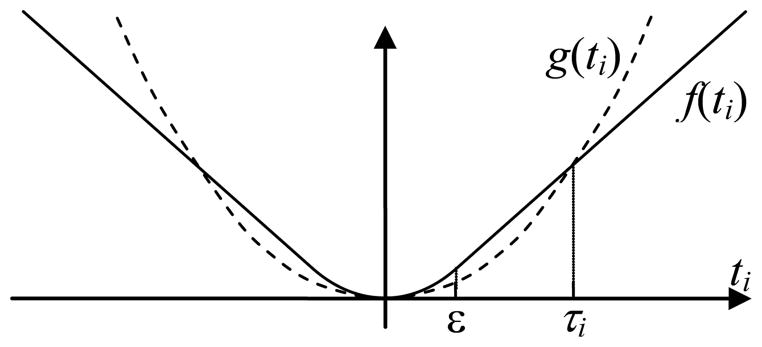
As illustrated in Figure 1, given a suitable operating point, τ, we approximate the modified norm using a quadratic function

Fig. 1.

Consider a prior image reconstruction that uses the modified norm that includes f(t_i). Finding a suitable operating point, τ_i, we may approximate f(t_i) with a quadratic function, g(t_i), that intersects at f(τ_i).

$$g\left(t_i\right)={\kappa }_i\left({\tau }_i\right)t_i^2{\kappa }_i\left({\tau }_i\right)=\{\begin{array}{ll}\frac{1}{2\epsilon }\hfill & \left|{\tau }_i\right|<\epsilon \hfill \\ \frac{\left|{\tau }_i-\frac{\epsilon }{2}\right|}{{\tau }_i^2}\hfill & \left|{\tau }_i\right|\ge \epsilon \hfill \end{array}$$ (12)

such that

$${\Vert t\Vert }^1\approx {\sum }_{i}g\left(t_i\right)={\left(t\right)}^T\mathbf{D}\left\{\kappa \left(\tau \right)\right\}\left(t\right).$$ (13)

Applying this approximation to (6) for the case of p_R = 1 and p_P = 1 yields an approximate decomposition:

$$\begin{array}{ll}\hfill F(y)& ={\left({\mathbf{A}}^T\mathbf{WA}+{\beta }_R{\mathbf{\Psi }}_R^T{\mathbf{D}}_R{\mathbf{\Psi }}_R+{\beta }_P{\mathbf{\Psi }}_P^T{\mathbf{D}}_P{\mathbf{\Psi }}_P\right)}^{-1}{\mathbf{A}}^T\mathbf{W}\widehat{l}\left(y\right)\hfill \\ \hfill G\left({\mu }_P\right)& ={\left({\mathbf{A}}^T\mathbf{WA}+{\beta }_R{\mathbf{\Psi }}_R^T{\mathbf{D}}_R{\mathbf{\Psi }}_R+{\beta }_P{\mathbf{\Psi }}_P^T{\mathbf{D}}_P{\mathbf{\Psi }}_P\right)}^{-1}·{\beta }_P{\mathbf{\Psi }}_P^T{\mathbf{D}}_P{\mathbf{\Psi }}_P{\mu }_P.\hfill \end{array}$$ (14)

It remains to choose an operating point for the approximation. In our analysis, we presume that the reconstruction in (3) has already been performed, allowing us to choose an operating point based on the solution, μ̂. This means the diagonal matrices in (14) may be defined as

$$\begin{array}{l}{\mathbf{D}}_R=\mathbf{D}\left\{\kappa \left({\mathbf{\Psi }}_R\widehat{\mu }\right)\right\}\\ {\mathbf{D}}_P=\mathbf{D}\left\{\kappa \left({\mathbf{\Psi }}_P\left(\widehat{\mu }-{\mu }_P\right)\right)\right\}.\end{array}$$ (15)

Note the close relation between (10) and (14) with equality if the diagonal matrices in (15) are identity. Moreover, it is straightforward to extend this methodology for other p-values. We note that the same decomposition may be applied to PICCS by leveraging the unconstrained form in (5). This necessitates setting W = I and choosing a sufficiently large β.

Since the system matrix is typically not computed explicitly and is too large to store, we adopt a conjugate gradient approach for approximating the terms F(y) and G(μ_P) in (14) to decompose a prior-image-based reconstruction (PIR-PLE or PICCS) into data- and prior-image-supported components.

III. Results/Discussion

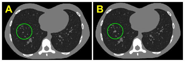
To investigate the data and prior image decomposition framework described in the previous section we adopted the imaging scenario illustrated in Figure 2. The experiment presumes the availability of a reconstructed prior image and data for a follow-up image that includes a change (viz., enlargement of a feature in the right lung). The follow-up acquisition involves highly sparse data. We investigate two acquisition strategies using a simulated C-arm geometry: 1) a region-of-interest (ROI) scan that acquires 60 laterally truncated projections over 360° (dashed white circle in Fig. 3); and 2) an angularly subsampled scan that acquires 20 untruncated projections over 360°. All experiments used 0.776 mm detector pixels, 0.8 mm isotropic voxels, and a monoenergetic x-ray beam with 10⁵ photons per detector element in the unattenuated beam. Both PIR-PLE and PICCS reconstructions are investigated.

Fig. 2.

Illustration of the prior image (A) and the true follow-up image (B) used to form current acquisition data (i.e., ROI or angularly undersampled). The images are the same except for the addition of a simulated lung nodule in the follow-up (green circle).

Fig. 3.

The information source decomposition applied to the ROI experiment using PIR-PLE. The two decomposition terms F(y) and G(μ_P) along with their sum (the predicted reconstruction, μ̂_D). The colorized source map combining F(y) and G(μ_P) in a single image conveys which features arise mainly from the prior image (red) and which arise largely from the newly acquired data (cyan/gray). The reconstruction is seen to rely more heavily on prior image information in regions outside the scanned region-of-interest (indicated by the dashed white circle).

We illustrate the application of the decomposition approach applied to the ROI acquisition experiment in Figure 3. A PIR-PLE reconstruction was formed, and both the data-based (F) and the prior-image-based (G) terms of the decomposition are shown. Moreover, the sum of the individual terms are presented as a check on the validity of the approximations leading to (9). (I.e., μ̂ ≈ μ̂_D which is qualitatively confirmed by the results.) A colorized information source map is also shown that identifies regions of the estimate that arise predominantly from either the current data (cyan/white) or the prior image (red). As one might expect, in this ROI scenario we see increasing contribution from the prior image in regions outside the scanned ROI. Moreover, the anatomical change (i.e., the simulated lung nodule) occurring between the prior image and follow-up can be clearly traced to the F term representing the newly acquired data.

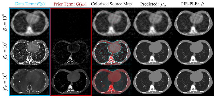
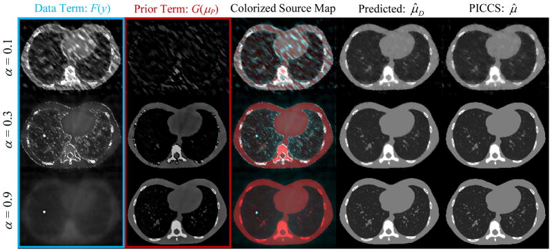
A second experiment considered the angularly undersampled case in which reconstructions were performed using both PIR-PLE and PICCS over a range of reconstruction parameters. Specifically, we performed a sweep over the prior image penalty strength (β_P) for PIR-PLE and a sweep of the α parameter in PICCS. The results are summarized in Figures 4 and 5, respectively. In both cases, the relationship between parameter strength and the strength of the prior image is clearly reflected in the decomposition. Moreover, the presence of the lung nodule is consistently represented in the data decomposition term, F. Interestingly, similar image reconstructions do not necessarily have similar decompositions – most evident in the reconstructions at higher levels of β_P and α. This suggests that even though the images appear very similar, they are actually relying on different sources of information transferred from the prior and newly acquired data, suggesting different conclusions regarding what might have changed in the image, and what is supported by the data.

Fig. 4.

Information source mapping applied to angularly undersampled data using PIR-PLE. Each row represents a different prior image penalty strength (β_P). The direct relationship between prior image penalty strength and the influence of the prior image is clear. Low β_P values result in a negligible G component and produce images similar to traditional penalized-likelihood with no prior image contribution. High β_P values yield greater similarity with the prior image, and the changes supported by the newly acquired data are readily apparent in the F component and the colorized source maps – most notably, the solitary lung nodule.

Fig. 5.

Information source mapping applied to the angular undersampling case and PICCS reconstruction. Each row represents a different choice of α, with larger α yielding increased reliance on the prior image and smaller α yielding increased reliance on the roughness penalty.

The ability to trace the source of information offers a potentially very important tool in beginning to understand how information propagates in prior-image-based reconstruction and how data and prior information are integrated in the resulting image. It also suggests a quantitative method by which one might justify the selection of penalty strengths and could even provide a basis by which one could design penalties that enforce a specific balance of information usage. Similarly, such a framework helps to illustrate the relationship between methods like PICCS and PIR-PLE and the particular information balance that is reached by either approach. Ongoing work includes analysis of such a relationship, the extent to which the information source map is quantitatively valid, and how such a framework could be implemented in systems employing prior-image-based reconstruction to communicate confidence levels to the observer that a perceived image feature arises from the prior or from the newly acquired data.

References

- 1.Chen GH, et al. Prior image constrained compressed sensing (PICCS): a method to accurately reconstruct dynamic CT images from highly undersampled projection data sets. Med Phys. 2008 Feb;35:660–3. doi: 10.1118/1.2836423. [DOI] [PMC free article] [PubMed] [Google Scholar]
- 2.Stayman J, et al. Penalized-likelihood reconstruction for sparse data acquisitions with unregistered prior images and compressed sensing penalties. SPIE Medical Imaging. 2011 [Google Scholar]
- 3.Thibault JB, et al. A three-dimensional statistical approach to improved image quality for multislice helical CT. Med Phys. 2007 Nov;34:4526–44. doi: 10.1118/1.2789499. [DOI] [PubMed] [Google Scholar]
- 4.Lange K. Convergence of EM image reconstruction algorithms with Gibbs smoothing. IEEE Trans Med Imaging. 1990;9:439–46. doi: 10.1109/42.61759. [DOI] [PubMed] [Google Scholar]
- 5.Ding Y, et al. Incorporation of Noise and Prior Images in Penalized-Likelihood Reconstruction of Sparse Data. SPIE Medical Imaging; San Diego, CA. 2012. [Google Scholar]
- 6.Fessler JA, Rogers WL. Spatial resolution properties of penalized-likelihood image reconstruction: space-invariant tomographs. IEEE Trans Image Process. 1996;5:1346–58. doi: 10.1109/83.535846. [DOI] [PubMed] [Google Scholar]
- 7.Sauer K, Bouman C. A Local Update Strategy for Iterative Reconstruction from Projections. Ieee Transactions on Signal Processing. 1993 Feb;41:534–548. [Google Scholar]