Statistical estimation of T₁ relaxation times using conventional magnetic resonance imaging

Abstract

Quantitative T₁ maps estimate T₁ relaxation times and can be used to assess diffusetissue abnormalities within normal-appearing tissue. T₁ maps are popular for studying the progression and treatment of multiple sclerosis (MS). However, their inclusion in standard imaging protocols remains limited due to the additional scanning time and expert calibration required and susceptibility to bias and noise. Here, we propose a newmethod of estimating T₁ maps using four conventional MR images, which are intensity-normalized using cerebellar gray matter as a reference tissue and related to T₁ using a smooth regression model. Using cross-validation, we generate statistical T₁ maps for 61 subjects with MS. The statistical maps are less noisy than the acquired maps and show similar reproducibility. Tests of group differences in normal-appearing white matter across MS subtypes give similar results using both methods.

1 Introduction

Quantitative magnetic resonance imaging (MRI) techniques are used to estimate features of human body tissue for the study of progression and treatment of diseases. For example, T₁ maps estimate T₁ relaxation times (T₁), which can be used as an indicator of inflammation and in nervous system tissue, demyelination, axonal loss and gliosis (Larsson et al., 1989; Vrenken et al., 2006). Increased relaxation times across normal-appearing white matter of the brain have been associated with a number of neurological diseases and disorders, including multiple sclerosis (MS), schizophrenia, alcoholism, optic neuritis, and near-terminal AIDS (Tofts and Du Boulay, 1990).

In MS, elevated T₁ relaxation times have been consistently observed in normal-appearing white matter (NAWM), relative to that of healthy control subjects (Bonnier et al., 2014; Castriota-Scanderbeg et al., 2004; Griffin et al., 2002; Parry et al., 2002; Vaithianathar et al., 2002; Vrenken et al., 2006). There is also evidence for elevated T₁ in MS patients in deep gray matter, particularly in the thalamus (Griffin et al., 2002; Parry et al., 2002; Vrenken et al., 2006), and in cortical gray matter (CGM) (Vrenken et al., 2006). Longitudinal studies have shown that the variance of T₁ in NAWM and CGM increases over time for MS patients (Davies et al., 2007; Manfredonia et al., 2007; Papadopoulos et al., 2010; Parry et al., 2003) and that average T₁ in NAWM may also increase (Manfredonia et al., 2007). Furthermore, T₁ is a clinically meaningful measure that contributes to a more complete picture of MS disease burden. In particular, the mean and variance of T₁ in NAWM have been found to be predictive of current and future disability (Manfredonia et al., 2007; Parry et al., 2002), and elevated T₁ in deep gray matter has been associated with fatigue (Neema et al., 2007; Niepel et al., 2006). Compared with lesion-based assessments of MS disease burden, which can be detected on standard clinical MR images, T₁ maps appear to provide complementary, not redundant, information (Griffin et al., 2002; Papadopoulos et al., 2010).

However, multiple factors have limited the widespread availability of T₁ maps. First, T₁ maps are still not included in most standard clinical or research protocols, due in part to the additional scanning time required for their acquisition. This is particularly true in the clinical setting, where limited resources and patient considerations typically restrict acquisition to conventional MR images. Second, many longitudinal studies of MS and other neurological diseases include years or even decades of imaging history, during only a fraction of which T₁ maps may have been acquired, thus limiting our understanding of the longitudinal evolution of T₁ in these diseases. Finally, T₁ mapping requires very careful scanner calibration, and many technical and environmental factors can introduce bias and noise, limiting reproducibility across acquisition methods, centers, scanners and visits.

In this paper, we introduce a novel method of computing T₁ maps based on conventional MR images. Traditional T₁ maps estimate T₁ analytically, using multiple (often two) T₁-weighted images acquired with different flip angles or inversion times to interpolate the T₁ relaxation curve (Blüml et al., 1993; Christensen et al., 1974; Crawley and Henkelman, 1988; Deoni, 2007; Henderson et al., 1999; Look and Locker, 1970; Messroghli et al., 2004). This curve is a non-linear function of T₁, a constant at a given physical location, and can be back-solved to estimate T₁. By contrast, our method estimates T₁ statistically using a voxel-wise regression model based on conventional MR images that are already included in many standard protocols. Using our method, a T₁ map can be estimated and added to a clinical or research study at any point following acquisition of the conventional MR images. A novel intensity normalization technique that utilizes the cerebellar gray matter as a reference tissue is key to the success of our method, Quantitative MR Estimation Employing Normalization (QuEEN). Henceforth, we refer to the traditional, analytically estimated T₁ maps as “T₁ maps” and to the QuEEN-estimated T₁ maps as “QuEEN maps”. The QuEEN model is fully automated and computationally efficient.

2 Methods

In this section, we detail the QuEEN method of T₁ estimation. QuEEN is comprised of two primary steps: intensity normalization of predictor MR images, followed by training of a flexible regression model relating the intensity-normalized predictor images to T₁. We use four predictor MR images that are routinely acquired in clinical and research protocols: T₁-weighted (T₁w), T₂-weighted (T₂w), proton density-weighted (PDw), and T₂-weighted fluid attenuated inversion recovery (FLAIR) images. These predictors were chosen due to their relatively wide availability and contribution to model performance. However, we also consider several alternative models based on subsets of these four predictors.

Prior to intensity normalization and model training, a standard MRI preprocessing pipeline is performed, including rigid registration (alignment) of images within each subject, removal of extracerebral voxels, and segmentation of brain tissue types. We validate the proposed methods by demonstrating that QuEEN maps are comparable to T₁ maps in terms of reproducibility and utility. Specifically, we illustrate that QuEEN maps can detect group differences in acute and diffuse white matter pathologies between subjects with different MS subtypes as well as, and possibly better than, T₁ maps, and we show that QuEEN and T₁ maps have similar measurement error rates.

2.1 QuEEN Model

2.1.1 Intensity Normalization

The MR images used as predictors in the QuEEN model are unitless, and therefore their intensities only have relative meaning within a scan. Intensity normalization of conventional MR images is often performed to introduce units and make intensities more comparable across images. By normalizing with respect to a reference region, intensities are converted to a measure of deviation from that reference, thus introducing meaningful units. For example, the z-score normalization method (Shinohara et al., 2011, 2014) estimates the center and variance of the distribution of intensities within a reference region, then normalizes the intensity of each voxel in the image by subtracting the center and dividing by the standard deviation; the resulting normalized intensities are therefore in units of standard deviations away from the center. For healthy subjects, NAWM is a useful reference region since it is well-imaged and easy to segment (Shinohara et al., 2014).

However, in many diseased populations, tissue damage occurs in NAWM that cannot be visually detected on contrast-based images; T₁ maps, which are sensitive to damage in normal-appearing tissue, are therefore often used to assess this damage. In order for QuEEN maps to possess this same property, a reference region that is minimally affected by disease—or that has low sensitivity on MRI to disease-related changes—should be chosen, so that the normalized intensities within NAWM reflect any tissue damage. Therefore, a good choice of reference region for the predictor images is vital. Candidate regions include cerebellar white and gray matter, cortical gray matter, deep gray matter, and cerebrospinal fluid (CSF). While CSF has the advantage of being generally unaffected by disease and has been used for normalization previously (Bakshi et al., 2002; Brass et al., 2006; Neema et al., 2009; Pujol et al., 1992; Tjoa et al., 2005; Van Waesberghe et al., 1998), we have found MR intensities within CSF to be very noisy. Therefore, normalization with CSF as a reference region tends to introduce variance into the normalized intensities and result in highly variable estimation of T₁ in the QuEEN model. Therefore, we do not recommend the use of CSF as a reference region in intensity normalization. Furthermore, in addition to NAWM, several other regions have been shown to be diffusely affected by MS, including cerebellar white matter (CBWM) (Bonnier et al., 2014; Casanova et al., 2003; Deppe et al., 2015), cortical gray matter (Kutzelnigg et al., 2005; Pirko et al., 2007; Vrenken et al., 2006) and deep gray matter (Griffin et al., 2002; Parry et al., 2002; Pirko et al., 2007; Vrenken et al., 2006).

Cerebellar gray matter (CBGM), on the other hand, has not been found to be diffusely affected by MS, and a recent investigation of T₁, T₂, $T_2^{\ast }$, and magnetization transfer ratio (MTR) in early-stage RRMS looked for but found no changes to CBGM (Bonnier et al., 2014). Furthermore, the cerebellum has been utilized previously as a reference region for intensity normalization of positron emission tomography (PET) in the contexts of MS (Ratchford et al., 2012) and Alzheimer’s disease (Kropholler et al., 2007), though to the best of our knowledge it has not been used for intensity normalization of MRI. We use cerebellar gray matter only, rather than the entire cerebellum, for two reasons: first, as mentioned above, CBWM may display diffuse disease-related changes in MS on MRI; second, the distribution of intensities in the cerebellum is a mixture of two distributions corresponding to gray and white matter respectively, and hence the center of the full distribution is sensitive to the relative volume of gray and white matter, which may differ across subjects.

We therefore propose a hybrid intensity normalization method using CBGM and NAWM. We propose using CBGM to estimate the center (e.g. median) in order to reflect disease-related changes in other tissue classes, including NAWM. Since we are primarily interested in detecting differences within and across subjects in the center of the distribution, we propose using NAWM to estimate the variance. NAWM is well-imaged and easy to segment, and thus this approach provides more stable variance estimation and more stable estimates of T₁. While changes to the variance of T₁ in NAWM have been documented, we have found this approach to improve accuracy of the QuEEN model, as it trades some bias for a greater reduction in variance. We now formally define the proposed intensity normalization procedure.

Let M_i(v) denote the raw intensity of voxel v for subject i in image M ∈ {FLAIR, PDw, T₁w, T₂w}. Using the z-score method, we normalize image M_i:

$$M_i^N(v)=\frac{M_i(v)-{\mu }_{i,M}^{(\mathit{CBGM})}}{{\sigma }_{i,M}^{(\mathit{NAWM})}},$$

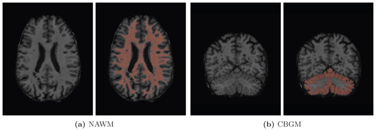
where ${\mu }_{i,M}^{(\mathit{CBGM})}$ is the median intensity within CBGM and ${\sigma }_{i,M}^{(\mathit{NAWM})}$ is the standard deviation of intensities within NAWM. We define the CBGM and NAWM regions using eroded versions of tissue class masks from an automated segmentation procedure, as described in Section 2.3.3. Though partial volume effects are common when segmenting cerebellar white and gray matter, erosion serves to mitigate these effects. Furthermore, the use of the median as the measure of center provides robustness against moderate segmentation errors, partial volume effects, and local abnormalities, such as lesions. Figure 1 shows the NAWM and CBGM regions for one randomly selected subject.

Figure 1.

NAWM and CBGM regions identified through minor erosion of automated tissue segmentation masks for one randomly selected subject. For each region, the slice containing the most voxels in the region of interest is displayed.

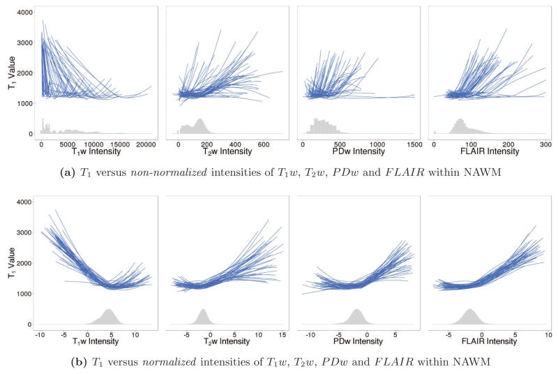
Figure 2 shows the relationships between T₁ and each predictor image before and after normalization. A histogram of the intensities across voxels from all subjects is also shown at the bottom of each plot. Each line is a smooth coefficient curve from a univariate generalized additive regression model (GAM) and estimates the relationship between T₁ and each predictor within a single subject and scanning session. The GAM model and its estimation are explained in more detail in Section 2.1.2. Intensity normalization aims to make these curves more similar across subjects and sessions, which will in turn lead to better out-of-sample prediction accuracy of T₁ for a cross-sectional regression model trained on multiple subjects. Figure 2b illustrates how the proposed intensity normalization method serves to standardize these curves across subjects and sessions, especially within the range of values visible on the histograms.

Figure 2.

T₁ versus non-normalized (a) and normalized (b) intensities of predictor images within NAWM. Each line is a smooth coefficient curve from a univariate GAM and estimates the relationship between T₁ and each predictor within a single subject and scanning session. The histogram of intensities across voxels from all subjects is also shown for each predictor image. Before intensity normalization, the relationships between T₁ and each predictor image varies greatly across subjects; after intensity normalization, the curves appear much more similar across subjects, especially within the range of values visible on the histograms. Furthermore, the relationships between T₁ and each predictor image are clearly nonlinear, motivating the use of a GAM regression approach.

2.1.2 Statistical Model

Following intensity normalization, a regression framework is used to estimate T₁ from the normalized predictor images. Specifically, we train the following generalized additive regression model (a smoothing spline model) for T₁ at voxel v in tissue class c for subject i:

$$T_{1i}(v)={\beta }_0^c+f_1^c(T_1{w}_i^N(v))+f_2^c(T_2{w}_i^N(v))+f_3^c({\mathit{PDw}}_i^N(v))+f_4^c({\mathit{FLAIR}}_i^N(v))+{\epsilon }_i(v),$$

where ${\epsilon }_i(v)\stackrel{\text{ind}}{\sim }N(0,{\sigma }_c^2)$, and the functions $f_j^c(·)$, j = 1, 2, 3, 4, are smooth population-level coefficient curves that map the normalized predictor image intensities in class c to deviations from the average T₁, represented by the intercept ${\beta }_0^c$. The curves shown in Figure 2 are simply estimated coefficient curves plus intercept for a set of single-subject, univariate GAMs. For any subject with a T₁w, T₂w, PDw and FLAIR image, T₁ at a given voxel within tissue class c can be estimated by applying the fitted regression curves ${\widehat{f}}_j^c(·)$, j = 1, 2, 3, 4, to the corresponding normalized predictor image intensities at that voxel, and summing them with the intercept term ${\widehat{\beta }}_0^c$.

We fit this model in the R statistical environment (version 3.0.2; R Core Team 2013) using the GAM function from the MGCV package (version 1.7-28; Wood 2006, 2011). This function represents the smooth curves as penalized regression splines. Generalized cross validation is used to estimate the degree of smoothness for each predictor, and the smoothing parameter estimation criterion is optimized using the Newton method (Gu and Wahba, 1991).

Several comments on this modeling framework are in order. First, a separate model is trained within each tissue class, because the relationship between the predictor image intensities and T₁ varies across classes. Second, the model assumes that the spatial dependence structure is explained entirely by the predictors, so that the residuals are spatially independent. Violation of this assumption will result in underestimation of the standard errors of the coefficient estimates, but will not likely have a strong effect on the coefficient estimates themselves (Liang and Zeger, 1986); as we rely on cross-validation error to quantify predictive performance, underestimation of the coefficient standard errors does not affect our results. Third, this is a cross-sectional, population-level model that treats all voxels from a group of subjects as independent observations. We chose a population-level model because we are primarily interested in assessing the marginal relationship between T₁ and the predictor images across subjects. This model is designed to produce the best estimate of T₁ for a subject for whom no T₁ map has been acquired; if subject-level information is available, a mixed-effects model may be more appropriate.

We also consider several more parsimonious model specifications. The full model relies on a 9-class tissue segmentation (see Section 2.3.3), which, while automated, is somewhat slow and may require tuning. As an alternative to the full tissue class segmentation, we can easily obtain a coarse segmentation consisting of white matter, gray matter and lesions using OASIS (Sweeney et al., 2013) to identify lesions and FSL FAST (Zhang et al., 2001) to identify normal-appearing white and gray matter. To assess the change in accuracy with this coarser segmentation, we create a set of pooled tissue class models by fitting a separate model for gray matter (CBGM, CGM, caudate, thalamus and putamen), non-lesion white matter (CBWM, NAWM and brainstem) and lesions, respectively. Furthermore, the full model requires the acquisition of four predictor images, some of which may not be acquired under every protocol; while T₁w images are routinely acquired, this is not always the case for T₂w/PDw (which are usually acquired simultaneously) and FLAIR images. To assess the importance of T₂w/PDw and/or FLAIR in the QuEEN model, we fit three separate submodels that include as predictors T₁w only, T₁w with T₂w and PDw, and T₁w with FLAIR.

2.2 Method Validation

We assess the performance of the QuEEN model using several criteria related to reproducibility and utility. To assess the reproducibility of QuEEN maps, we compute estimation error and prediction error. We define the estimation error of a QuEEN map at each voxel as the difference between the intensities on the QuEEN map and T₁ map from the same session. We note that the regression framework used to generate QuEEN maps may serve to reduce the noise typically found on T₁ maps due to the “shrinkage effect” of regression, in which observations are pulled towards the mean, an effect that has previously been shown to improve reproducibility of functional MRI measures (Mejia et al., 2015; Shou et al., 2014).

While estimation error is useful, it is difficult to determine what constitutes a good or bad estimation error without knowing the measurement error of T₁ maps. Therefore, we also define prediction error as the difference at each voxel between a T₁ or QuEEN map and a second T₁ map acquired at a later date. We compute the prediction error of the T₁ and QuEEN maps of those subjects in our dataset for whom a second T₁ map is available. Note that while prediction error may be affected by real biological changes, such as disease progression, those changes will affect the prediction errors of T₁ and QuEEN maps similarly, and hence they can be compared fairly.

For each error rate, we compute the cross-validated root median squared error (CV-rMSE) of each QuEEN map by tissue class. It is important to note that, due to measurement error inherent in T₁ maps and the possibility for such errors to be spatially recurrent across multiple scans, the prediction error of T₁ maps may be somewhat underestimated.

To assess the utility of QuEEN maps, we use both QuEEN maps and T₁ maps to detect acute and diffuse changes in white matter, a common use of T₁ maps. Specifically, we perform Wilcoxon tests of group differences in median T₁ within NAWM and lesions between different MS subtypes. Previous work suggests that secondary-progressive MS (SPMS) subjects show elevated T₁ in NAWM relative to relapsing-remitting MS (RRMS) and primary-progressive MS (PPMS) patients, and that RRMS patients show elevated T₁ in NAWM relative to PPMS patients (Vrenken et al., 2006). Therefore, for each of these pairs we conduct a one-sided test for differences in median NAWM T₁. Much extant literature also finds that patients with MS show elevated T₁ relative to healthy volunteers (HVs) (Griffin et al., 2002; Miller et al., 1989; Parry et al., 2002, 2003; Vaithianathar et al., 2002; Vrenken et al., 2006). We therefore also conduct a one-sided test for differences in median NAWM T₁ for MS patients overall and each MS subtype versus HVs. However, as our HV group is very small, we present these results as preliminary findings in Appendix Figure B.2. Finally, we also perform a two-sided test for differences in median lesion T₁ between each pair of MS subtypes.

2.3 Materials

2.3.1 Study Population

Our dataset consists of MRI studies collected from 75 subjects. In order to ensure image quality for model training and validation, we performed careful quality control and excluded four studies due to subject motion, two due to registration problems, five due to tissue class segmentation errors, and two due to bias in the T₁ map. The 62 remaining studies include 29 PPMS patients, 15 RRMS patients,16 SPMS patients, and 2 HVs. Additional summary statistics are shown in Table 1. For model training, we formed a high-quality dataset containing 45 studies by excluding any studies where even minor segmentation errors or subject motion were present. For model validation we generated QuEEN maps for all 62 studies, as described in Section 2.3.4.

Table 1.

Summary statistics for healthy volunteers (HVs), primary-progressive MS (PPMS) patients, relapsing-remitting MS (RRMS) patients, and secondary-progressive MS (SPMS) patients.

	HV	PPMS	RRMS	SPMS
n	2	29	15	16
% Female	50%	55%	87%	44%
Mean Age (sd)	24 (0.6)	56 (7.4)	45 (13.8)	53 (7.5)
Mean Disease Duration (sd)	NA	13.6 (9.4)	8.2 (6.8)	24.7 (9.1)
Median EDSS (range)	NA	6.0 (2.0–7.5)	1.5 (1.0–6.0)	6.5 (1.5–7.0)

To assess prediction error, a second MRI study was collected for 36 subjects. Of these, we excluded one study due to motion and two due to segmentation errors. The remaining 33 studies include 20 PPMS patients, 12 SPMS patients, and one RRMS patient. The average length of time between the two studies is 169 days and ranges from 21 to 301 days.

2.3.2 Image Acquisition

Each MRI study includes the following images, all collected on a Siemens Skyra 3 Tesla (3T) scanner: a T₁ map, acquired as two T₁-FLASH (Fast Low Angle SHot) sequences at differing flip angles [TR=7.8ms, TE=3ms, FA=3/18] (Christensen et al., 1974; Gupta, 1977) with a B₀+B₁ field map for FA correction (Duan et al., 2013); a T₁w-MPRAGE (Magnetization-Prepared RApid Gradient Echo) image [TR=3000ms, TE=3.03ms, TI=900ms, FA=9]; PDw and T₂w images from a dual-echo turbo spin echo (TSE) sequence [TR=3000ms, TE=11ms/101ms, FA=150, ETL=14]; and a 3D T₂-weighted FLAIR image acquired using a T₂-selective inversion pulse optimized for T₂ of 120ms [TR=4800ms, TE=354ms, TI=1800ms, Variable FA]. All scans were acquired at 1.0mm isotropic resolution except the PDw/T₂w TSE sequence, which was acquired at 0.93 × 0.93 × 3.0mm resolution.

2.3.3 Image Preprocessing & Tissue Segmentation

For the T₁ map of each subject, we perform B₀-field correction to reduce magnetic field inhomogeneity and B₁-field correction to account for the radio-frequency (RF) transmit bias field. B₀ correction is required as it causes a shift in center frequency. B₁ is calculated by using off-resonance RF pulse preparations symmetric to the water excitation frequency, as detailed in Sacolick et al. (2010). Further modification of this technique is required to obtain the B₁ map from the entire brain in a reasonable scan time due to SAR (specific absorption rate) limitations at 3T; the B₁ correction pulse sequence we use is detailed in Duan et al. (2013).

For each subject, we rigidly align the corrected T₁ map and T₁w, T₂w, PDw and FLAIR images to the Montreal Neurological Institute (MNI) 152 1.0 mm nonlinear template, using a two-step registration technique where the second alignment is done after skull-stripping. We apply the N4 inhomogeneity correction algorithm (Tustison et al., 2010) to the T₁w, T₂w, PDw and FLAIR images, and we remove extracerebral voxels using the SPECTRE skull-stripping algorithm (Carass et al., 2011).

For each study, we use a tissue class segmentation from Topology Preserving Anatomy Driven Segmentation (TOADS) (Bazin and Pham, 2006) for HVs and Lesion-TOADS (Shiee et al., 2010) for patients with MS. Both algorithms identify eight tissue classes (cerebral white matter, cortical gray matter, cerebellar white matter, cerebellar gray matter, caudate, thalamus, putamen and brainstem) and CSF; Lesion-TOADS also identifies white matter lesions. Since TOADS and Lesion-TOADS employ topological constraints that can cause segmentation errors within the ventricles, which sometimes appear discontinuous on MRI, we correct the ventricular segmentation using the non-topologically constrained maximum membership classes.

To create a brain mask including only tissue, we exclude voxels identified as CSF on the tissue class segmentation. Furthermore, we exclude any voxels that appear hypointense in the FLAIR image by thresholding the image below the 80th percentile, which has been used to to help correct for CSF segmentation errors (Sweeney et al., 2013). In cases where the brain mask extended beyond the field of view of an image because of the angulation of one of the acquisitions, voxels outside of this field of view were excluded in all sequences. Finally, we exclude any voxels with physically implausible T₁ for brain tissue (less than zero or greater than 5000 ms). The remaining voxels comprise the brain mask.

To create a conservative mask of each tissue class, we start with the tissue class segmentation described above and remove any voxels outside of the brain mask. To exclude voxels exhibiting partial volume effects along tissue class borders, we erode the mask of each tissue class using a 3×3×3 diamond-shaped kernel. Eroded voxels are excluded from model training and validation measures, but are included for whole-image prediction.

While processing times vary significantly across subjects, the total processing time for each subject is approximately 1–1.5 hours on a single core of a 2.30GHz Intel(R) Xeon(R) CPU E7-4870 v2 processor. The major computational steps are coregistration (30–40 minutes), skull stripping (20–30 minutes), and tissue segmentation (20–40 minutes). T₁ map calculation takes approximately 3 minutes, and all other steps are negligible in time. Many of the processing steps can be performed for multiple subjects in parallel. Quality control was performed by one expert neuroradiologist and two statisticians with experience in structural MRI, and takes approximately 2 minutes per scanning session in total.

2.3.4 QuEEN Map Generation

Within the high-quality dataset, we generate QuEEN maps through leave-one-subject-out cross-validation. That is, for each subject, the QuEEN statistical model is fit on all other subjects in the high-quality dataset, and the resulting model is used to generate the QuEEN map for that subject. For subjects not included in the high-quality dataset, QuEEN maps are generated using the QuEEN statistical model trained on all subjects in the high-quality dataset. The results reported below are based on the high-quality dataset; results including the full dataset are shown in Appendix Figures C.3–C.5.

3 Results

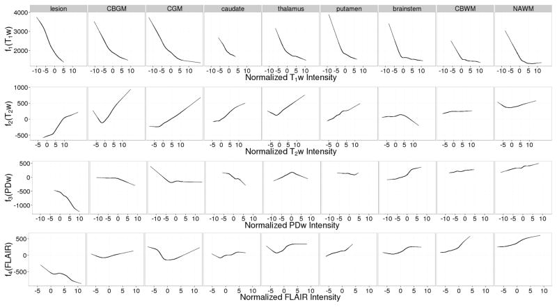
Figure 3 shows the estimated GAM coefficient curves within each tissue class. The curves for T₁w appear similar across tissue classes, while the curves for T₂w, PDw and FLAIR vary markedly across classes. This may signify that T₁w captures general characteristics of the T₁ map, while the other predictor images capture more subtle features within each tissue class.

Figure 3.

Estimated coefficient curves for the generalized additive regression model within each tissue class. The estimated intercept is included in the T₁w curves to illustrate global differences between tissue classes. For a given tissue class and predictor image, the value of the coefficient function evaluated at a particular (normalized) image intensity is the amount (in ms) that a voxel in that class with that intensity contributes to the predicted T₁ value.

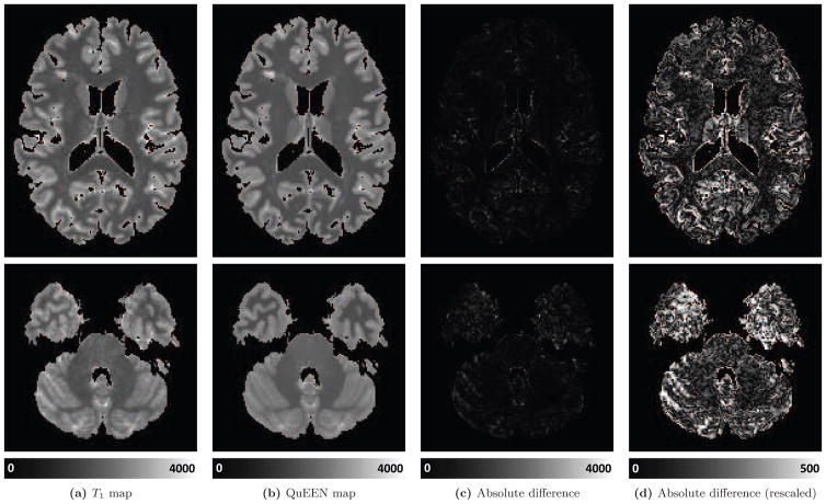
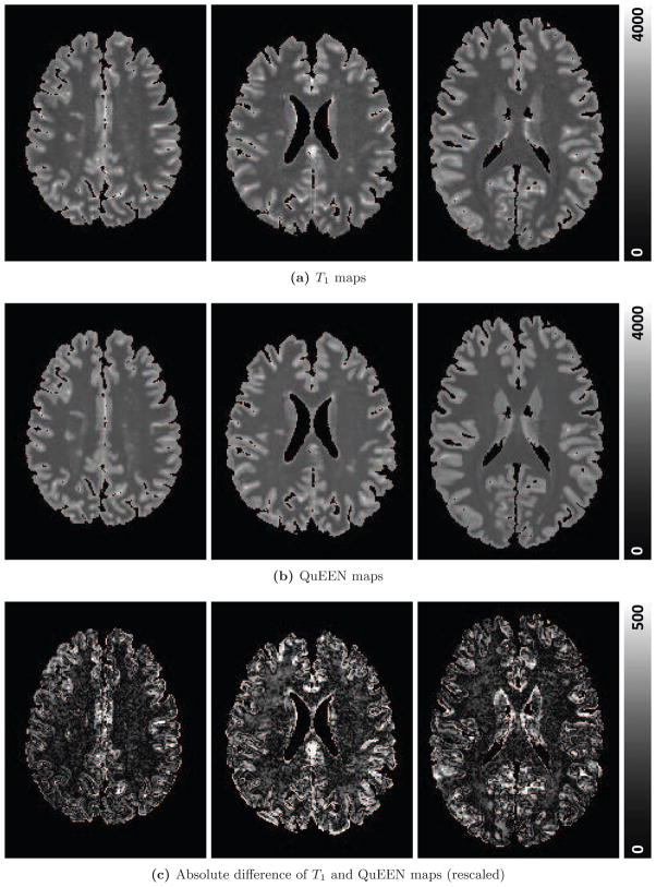
Figure 4 shows, for one randomly selected subject, two axial slices of the T₁ map (Figure 4a), QuEEN map (Figure 4b), and the magnitude of the difference between them. The difference image is shown on the same scale as the images (Figure 4c) and again on a different scale to show greater detail (Figure 4d). The T₁ and QuEEN maps appear very similar; however, the QuEEN map appears smoother and contains less noise on the border between brain tissue and cerebrospinal fluid (CSF). The subject displayed is an RRMS patient; example images from subjects with PPMS and SPMS and a HV are shown in Appendix Figure A.1.

Figure 4.

For one randomly selected example subject with RRMS, two axial slices of the T₁ map (a), QuEEN map (b), and the absolute value of the difference between the two on the same scale as the images (c) and rescaled to show greater detail (d) are shown.

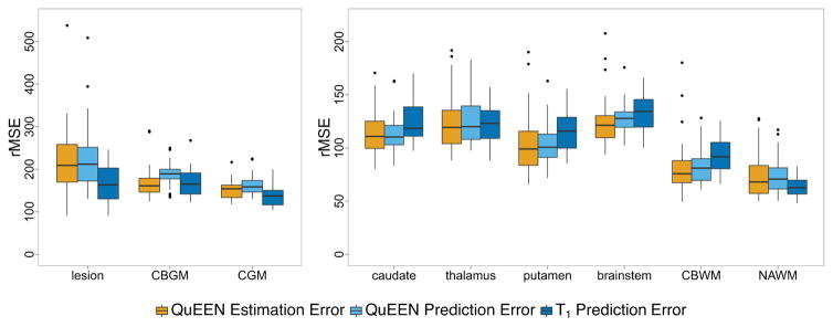
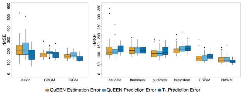
Figure 5¹ shows boxplots over subjects of the QuEEN estimation error (shown in orange), QuEEN prediction error (shown in light blue), and T₁ prediction error (shown in dark blue) within each tissue class, in terms of CV-rMSE. The reproducibility of QuEEN and T₁ maps appear quite similar overall, with differences within certain tissue classes. In particular, the QuEEN maps appear to be more reproducible in deep gray matter (thalamus, caudate and putamen), CBWM and the brainstem, while the T₁ maps tend to be more reproducible in CGM, CBGM, NAWM and lesions.

Figure 5.

For each tissue class, boxplots of the QuEEN estimation error (shown in orange), QuEEN prediction error (shown in light blue), and T₁ prediction error (shown in dark blue). Each error rate is summarized as the CV-rMSE over all voxels in the eroded mask of each tissue class for a single subject. The boxplots of QuEEN estimation error show the distribution over all subjects in the high-quality dataset, while the boxplots of QuEEN and T₁ prediction errors show the distribution over those subjects in the high-quality dataset who received a second scan. The reproducibility of QuEEN and T₁ maps appear quite similar overall, with differences within certain tissue classes.

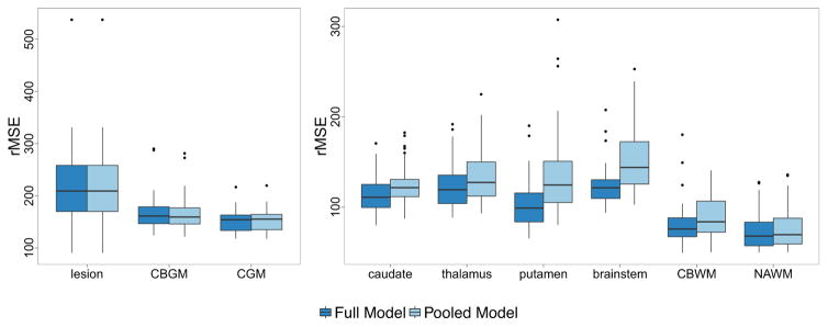
Figure 6 shows boxplots of the QuEEN estimation error for the fully stratified model and the pooled tissue class model. A moderate loss of accuracy is seen in the caudate, thalamus, putamen, brainstem and CBWM, while a small loss of accuracy can be seen in NAWM. A disproportionate loss of accuracy is not surprising when smaller classes are pooled with larger classes, since the coefficient estimates will be pulled towards the majority of the observations. Within NAWM, a paired t-test for the change in CV-rMSE for the pooled model versus the fully stratified model shows that the pooled model does result in a small but statistically significant loss of accuracy, with an increase in CV-rMSE of 3.02 ms (p = 4.2 × 10⁻¹¹, 95% CI [2.27, 3.78]) per subject. This illustrates that while accuracy is clearly lost in some tissue classes, if NAWM is of primary interest the pooled tissue class model based on a basic tissue class segmentation can be used to estimate T₁ in NAWM almost as accurately.

Figure 6.

For each tissue class, boxplots of the QuEEN estimation error for the fully stratified model (9 tissue classes) and pooled model (3 tissue classes), using the high-quality dataset. Each error rate is summarized as the CV-rMSE over all voxels in the eroded mask of each tissue class for a single subject.

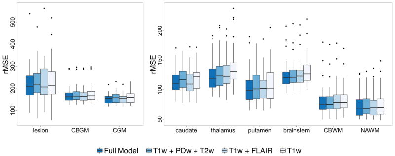
Figure 7 shows boxplots of the QuEEN estimation error for the full model and for the three models with fewer predictors. When FLAIR is excluded, a minor reduction in accuracy is apparent in lesions and gray matter (cortical, deep and cerebellar), while when T₂w and PDw are excluded we observe a small loss of accuracy in CBWM, NAWM and the brainstem. A series of paired t-tests for the change in CV-rMSE within NAWM show that each submodel results in a very small but statistically significant loss of accuracy, with an increase in rMSE of 1.20 ms (p = 0.009, 95% CI [0.31, 2.09]) per subject when FLAIR is excluded, 0.64 ms (p = 0.024, 95% CI [0.09, 1.20]) when T₂w and PDw are excluded, and 2.83 ms (p = 0.0002, 95% CI [1.40, 4.27] when all three are excluded. While accuracy can clearly be maximized by including all four predictors, the loss of accuracy if one or more of the secondary predictors is not available is small.

Figure 7.

For each tissue class, boxplots of the QuEEN estimation error for the full model and three submodels, using the high-quality dataset. Each error rate is summarized as the CV-rMSE over all voxels in the eroded mask of each tissue class for a single subject.

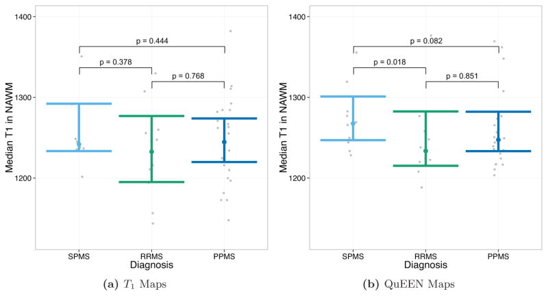
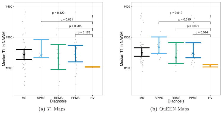
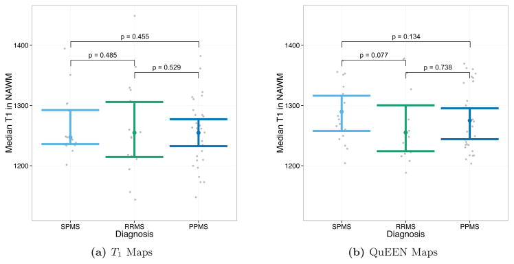
Figures 8 and 9 show the results of tests of group differences between disease types. Figure 8 shows the median T₁ in NAWM as estimated by T₁ maps (Figure 8a) and QuEEN maps (Figure 8b). For each pair of groups, the p-value shown on the plot corresponds to a one-sided Wilcoxon test that the group on the left has a greater median than the group on the right. As described in Section 2.2, these comparisons were chosen based on previous findings. Surprisingly, while none of the expected differences are significant based on T₁ maps, based on QuEEN maps SPMS patients show a significant or marginally significant increase compared to RRMS patients (p = 0.018) and PPMS patients (p = 0.082).

Figure 8.

Tests of group differences in median NAWM T₁ based on (a) T₁ maps and (b) QuEEN maps, using the high-quality dataset. Each point represents a single subject, and the confidence bars indicate Wilcoxon 95% intervals for the median across subjects in each patient group. The p-value for each pair of groups corresponds to a one-sided Wilcoxon test that the group on the left has a greater median than the group on the right. For example, the test of SPMS > RRMS has p = 0.378 using T₁ maps and p = 0.018 using QuEEN maps.

Figure 9.

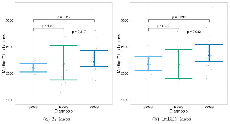
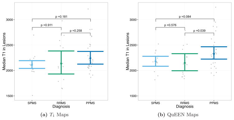
Tests of group differences in median lesion T₁ based on (a) T₁ maps and (b) QuEEN maps, using the high-quality dataset. Each point represents a single subject, and the confidence bars indicate Wilcoxon 95% intervals for the median across subjects in each patient group. The p-value for each pair of groups corresponds to a two-sided Wilcoxon test for difference in medians. While no differences are significant based on T₁ maps, two differences are marginally significant based on QuEEN maps: PPMS ≠ RRMS (p = 0.039) and PPMS ≠ SPMS (p = 0.084).

Figure 9 shows the median T₁ in lesions as estimated by T₁ maps (Figure 9a) and QuEEN maps (Figure 9b). For each pair of groups, the p-value shown on the plot corresponds to a two-sided Wilcoxon test for a difference in medians. We perform two-sided tests because we do not have strong a-priori beliefs about differences in lesion T₁ between disease types. While none of the differences are significant based on T₁ maps, using QuEEN maps PPMS patients show a marginally significant difference with both RRMS patients (p = 0.082) and SPMS patients (p = 0.092). In both cases, the estimate of the median is higher for PPMS patients. This finding is supported by earlier work that identified indicators of increased gliosis and axonal loss in PPMS lesions relative to RRMS lesions (Suhy et al., 2000).

These results suggest that QuEEN maps can be used in place of T₁ maps for group difference analyses. Regarding power, while these results are too preliminary to conclude definitively that QuEEN maps are more powerful for tests of group differences, median T₁ in NAWM and lesions estimated using QuEEN maps appear to exhibit smaller within-group variance—suggested by slightly narrower confidence bands and fewer outliers in each group—which would tend to result in more powerful tests.

4 Discussion

In this paper, we have proposed QuEEN, a new method for estimating T₁ relaxation times that only requires the acquisition of a T₁w image and up to three other conventional MR images. We have demonstrated the reproducibility of QuEEN maps by showing that they have similar prediction error compared with T₁ maps and, in fact, have improved reproducibility in deep gray matter. Given the emerging recognition of the importance in MS of the thalamus (Haider et al., 2014; Minagar et al., 2013; Zivadinov et al., 2013), this may represent an important advancement in the study of MS. Furthermore, we have demonstrated the utility of QuEEN maps for group comparisons, as tests of group differences of T₁ in NAWM and lesions using QuEEN maps resulted in similar findings as those same tests performed using T₁ maps.

While the majority of the information in the QuEEN model is derived from the T₁w images (see Figure 3), the inclusion of T₂w and FLAIR improves the accuracy of T₁ estimation due to the statistical association between T₂ and T₁ in brain tissue. Our flexible modeling framework allows for the contribution of T₂w and FLAIR intensities to be stronger in regions where there is a stronger association between T₁ and T₂. In this way, the model leverages all the available information in the multisequence predictor images in order to produce the best possible estimate of T₁ at each location. While the biophysical interpretation of QuEEN maps is lacking in abstraction, QuEEN maps can be interpreted in terms of their estimation of T₁.

The novel intensity normalization procedure we propose, which is key to the accuracy of the QuEEN model, uses cerebellar gray matter to estimate the “center” of the distribution of image intensities. We also evaluated several other tissue types for this purpose, including NAWM, CSF, and extra-cerebral soft tissue, and we found CBGM to demonstrate the best performance by far (results not shown). We believe this is due to the combination of its relatively high similarity across subjects (compared with NAWM) and relatively low noise (compared with CSF and extra-cerebral soft tissue). However, there are some potential issues to consider before employing this normalization approach. First, CBGM can exhibit some changes due to MS disease pathology (Howell et al., 2014). From an imaging point of view, these changes may be small and localized in MS, but for patients with other neurological diseases in which CBGM may be affected to a larger degree, the choice of reference region should be revisited before generating QuEEN maps. Second, the cerebellum is close to the receive coil array, and is hence more susceptible to bias-field inhomogeneities. Finally, segmentation of gray and white cerebellar tissue is required. However, this segmentation is not required to be perfect, as the methods we propose are designed to be robust to partial volume effects and minor segmentation errors.

QuEEN uses a full 9-class tissue segmentation. The methods currently available for segmentation in diseased populations require tuning and are prone to errors, even when applied by an expert technician. In fact, several of the subjects in our dataset were excluded due to problems with the tissue class segmentation, illustrating the need for better segmentation methods for diseased populations. To account for small errors and partial volume effects, we use eroded tissue class masks for intensity normalization and model training. Alternatively, we have demonstrated that a coarser segmentation (gray matter, non-lesion white matter and lesions) can replace the full segmentation with minor loss of model accuracy within large tissue classes, such as NAWM. However, it is still necessary to estimate the “center” of the distribution of intensities within CBGM for the purposes of intensity normalization. In the absence of a full tissue class segmentation, histogram “stripe”-based methods such as that described in Shinohara et al. (2014) can be adapted to estimate the median intensity within CBGM and standard deviation within NAWM.

Our results demonstrate that QuEEN map reproducibility varies across tissue classes. In particular, we observe lower reproducibility in lesions. The decreased performance of the QuEEN model in lesions may be due in part to the heterogeneity of the lesion class, as different types of lesions exhibit distinct pathological conditions and associations between T₁ and T₂. Segmentation or labelling of multiple lesion classes would allow for separate model fits within each class, customized to the class-specific relationship between T₁ and each predictor image. In the context of a single lesion class, an extension to the modeling framework that may improve model fit within lesions is bivariate (surface) smoothing of the coefficients. Bivariate smoothers, as opposed to the univariate smoothers utilized in this paper, are more computationally demanding but allow for a more flexible model fit, which may be able to better adapt to the heterogeneity within the lesion class.

The QuEEN model can be applied using coefficient estimates based on external data or can be retrained to produce a center-specific model. The choice depends both on the research objectives and characteristics of the predictor images. If the objective is to use QuEEN maps to supplement existing T₁ maps that have been previously acquired, then a center-specific model may be needed to maximize comparability of the QuEEN maps and acquired T₁ maps. However, if comparability with acquired T₁ maps is not a concern and similar predictor images are available, our model estimates can be used to generate QuEEN maps at different centers. Furthermore, if the objective is to compare T₁ across multiple centers, QuEEN maps generated from a single training model may actually be more reproducible across centers than acquired T₁ maps, which may be subject to center-to-center biases. In that case, training a center-specific model would be detrimental, as it would translate any center-to-center biases to the QuEEN maps.

One additional consideration is the availability and acquisition protocols of the predictor images. If the four predictor images used in our modeling framework are not all available, highly accurate QuEEN maps can still be produced as long as a sufficiently high-contrast and high-resolution T₁w image is available. In particular, as acquisition type determines the contrast between different tissue types, the effect of different acquisition types of the predictor images, such a T₁w-FSPGR (Fast SPoiled Gradient Echo) versus a T₁w-MPRAGE, would need to be explored carefully. In this study we have utilized a high-resolution (1 mm isotropic) T₁w-MPRAGE image; it remains to be explored whether QuEEN maps can be reliably constructed using lower-quality or lower-resolution T₁w images, such as those collected in many clinical and some research settings, or those available in historical studies. The T₁w and other predictor images used should have sufficiently high resolution such that cerebellar gray matter can be segmented.

One limitation of the current study is that it is based upon data acquired at a single center on the same scanner and protocol and only includes a small number of healthy volunteers. Future multi-center studies of QuEEN including large numbers of patients and healthy volunteers are necessary to understand and validate the center-to-center reproducibility of QuEEN, and to assess the robustness of the model to differences in the image acquisition protocols of the predictor images.

An advantage of the QuEEN model is that it treats each individual voxel as a separate, independent observation and hence does not require spatial normalization across subjects. As diseased brains can be difficult to normalize to a template (Eloyan et al., 2014), avoiding this step is a strength of our approach. While the QuEEN regression residuals may in truth exhibit some spatial correlation, this does not affect the validity of our results, as we rely on cross-validation error rather than standard errors of model coefficients to evaluate model fit.

QuEEN is a flexible model framework that can be extended to other quantitative modalities. Future directions will explore the potential of the QuEEN model to estimate other image types, including T₂*. QuEEN maps may also be useful for the study of diseases other than MS where T₁ is an important biomarker, including Parkinson’s disease, cancers, and diseases of the heart, lungs, and abdomen. The intensity normalization procedure is key to the accuracy of the QuEEN model and should be adapted to each context by identifying a region that is minimally affected by the disease in question and is relatively well imaged. For example, in the presence of a high white matter lesion load, such as in small vessel disease, CADASIL, or Alzheimer’s disease, it may be difficult to reliably segment NAWM. In these cases, it may be necessary to identify a different tissue class, such as CBGM, to estimate the variance for intensity normalization. Future research should focus on assessing accuracy of QuEEN maps for different patient populations.

5 Conclusion

In this paper, we have proposed a new way to estimate T₁ relaxation times retroactively that only requires the acquisition of four or fewer conventional MR images. The “QuEEN maps” produced using these methods were shown to have similar accuracy and reliability compared with traditional acquired T₁ maps. Furthermore, QuEEN maps offer several advantages over traditional T₁ maps. Of primary importance is convenience and retroactive availability: QuEEN maps can be computed without any additional scan time using four or fewer conventional images. Since these images have historically been included in most clinical and research protocols, our method has the potential to greatly increase the availability of T₁ maps for clinical and research use. Furthermore, QuEEN maps can be used in place of traditional T₁ maps for tests of differences in T₁ between MS subtypes in NAWM and lesions. Further research is needed to validate QuEEN across centers, scanners, protocols and populations.

Highlights.

• We introduce a statistical model for estimation of T1 based on conventional MRI.

• The proposed methods avoid traditional T1 map acquisition techniques.

• Statistical T1 maps are less noisy than acquired maps and similar in reliability.

• Group differences in T1 are similar, but statistical T1 maps may be more powerful.

• The proposed method has the potential to greatly increase T1 map availability.

A Example images and difference images

Figure A.1.

For three randomly selected subjects, one axial slice of the T₁ map (a), the QuEEN map (b), and the absolute value of the difference between the two on a different scale (c) are shown. The first column shows a subject with SPMS, the middle column shows a subject with PPMS, and the third column shows a healthy volunteer.

B Tests of group differences with healthy controls

Figure B.2.

Exploratory tests of group differences in NAWM between MS groups and healthy volunteers using T₁ maps (a) and QuEEN maps (b), using the high-quality dataset. Each point represents a single subject, and the confidence bars indicate Wilcoxon 95% (50% for the HV group) intervals for the median across subjects in each patient group. The p-value for each pair of groups corresponds to a one-sided Wilcoxon test that the patient group has a greater median than the HV group. Using T₁ maps, only the SPMS group shows a marginally significant elevation in NAWM T₁ relative to HVs (p = 0.061). However, using QuEEN maps, each patient group shows a significant or marginally significant elevation in NAWM T₁ relative to HVs.

C Results on full validation set

Figure C.3.

For each tissue class, boxplots of the QuEEN estimation error (shown in orange), QuEEN prediction error (shown in light blue), and T₁ prediction error (shown in dark blue), using the full dataset. Each error rate is summarized as the CV-rMSE over all voxels in the eroded mask of each tissue class for a single subject. The boxplots of QuEEN estimation error show the distribution over all subjects, while the boxplots of QuEEN and T₁ prediction error show the distribution over those subjects who received a second scan. We see more outliers compared with Figure 3, but the relationship between the error rates in each tissue class remains relatively unchanged.

Figure C.4.

Tests of group differences in median NAWM T₁ using (a) T₁ maps and (b) QuEEN maps, using the full dataset. Each point represents a single subject, and the confidence bars indicate Wilcoxon 95% intervals for the median across subjects in each patient group. The p-value for each pair of groups corresponds to a one-sided Wilcoxon test that the group on the left has a greater median than the group on the right. While no differences are significant based on T₁ maps, based on QuEEN maps SPMS patients show a marginally significant increase in NAWM T₁ relative to RRMS patients (p = 0.077).

Figure C.5.

Tests of group differences in median lesion T₁ using (a) T₁ maps and (b) QuEEN maps, using the full dataset. Each point represents a single subject, and the confidence bars indicate Wilcoxon 95% intervals for the median across subjects in each patient group. The p-value for each pair of groups corresponds to a two-sided Wilcoxon test for difference in medians. While no differences are significant based on T₁ maps, two differences are significant or marginally significant based on QuEEN maps: PPMS > RRMS (p = 0.039) and PPMS > SPMS (p = 0.084).

References

- Bakshi R, Benedict RH, Bermel RA, Caruthers SD, Puli SR, Tjoa CW, Fabiano AJ, Jacobs L. T2 hypointensity in the deep gray matter of patients with multiple sclerosis: a quantitative magnetic resonance imaging study. Archives of Neurology. 2002;59(1):62. doi: 10.1001/archneur.59.1.62. [DOI] [PubMed] [Google Scholar]
- Bazin P-L, Pham DL. TOADS: topology-preserving, anatomy-driven segmentation. Proceedings of the 2006 IEEE International Symposium on Biomedical Imaging; 2006. pp. 327–330. [Google Scholar]
- Blüml S, Schad LR, Stepanow B, Lorenz WJ. Spin-lattice relaxation time measurement by means of a TurboFLASH technique. Magnetic Resonance in Medicine. 1993;30(3):289–295. doi: 10.1002/mrm.1910300304. [DOI] [PubMed] [Google Scholar]
- Bonnier G, Roche A, Romascano D, Simioni S, Meskaldji D, Rotzinger D, Lin YC, Menegaz G, Schluep M, Du Pasquier R, et al. Advanced MRI unravels the nature of tissue alterations in early multiple sclerosis. Annals of Clinical and Translational Neurology. 2014;1(6):423–432. doi: 10.1002/acn3.68. [DOI] [PMC free article] [PubMed] [Google Scholar]
- Brass S, Benedict RH, Weinstock-Guttman B, Munschauer F, Bakshi R. Cognitive impairment is associated with subcortical magnetic resonance imaging grey matter T2 hypointensity in multiple sclerosis. Multiple Sclerosis. 2006;12(4):437–444. doi: 10.1191/135248506ms1301oa. [DOI] [PubMed] [Google Scholar]
- Carass A, Cuzzocreo J, Wheeler MB, Bazin PL, Resnick SM, Prince JL. Simple paradigm for extra-cerebral tissue removal: Algorithm and analysis. NeuroImage. 2011;56(4):1982–1992. doi: 10.1016/j.neuroimage.2011.03.045. [DOI] [PMC free article] [PubMed] [Google Scholar]
- Casanova B, Martinez-Bisbal M, Valero C, Celda B, Marti-Bonmati L, Pascual A, Landente L, Coret F. Evidence of Wallerian degeneration in normal appearing white matter in the early stages of relapsing-remitting multiple sclerosis. Journal of Neurology. 2003;250(1):22–28. doi: 10.1007/s00415-003-0928-0. [DOI] [PubMed] [Google Scholar]
- Castriota-Scanderbeg A, Fasano F, Filippi M, Caltagirone C. T1 relaxation maps allow differentiation between pathologic tissue subsets in relapsing-remitting and secondary progressive multiple sclerosis. Multiple Sclerosis. 2004;10(5):556–561. doi: 10.1191/1352458504ms1073oa. [DOI] [PubMed] [Google Scholar]
- Christensen KA, Grant DM, Schulman EM, Walling C. Optimal determination of relaxation times of Fourier transform nuclear magnetic resonance. determination of spin-lattice relaxation times in chemically polarized species. The Journal of Physical Chemistry. 1974;78(19):1971–1977. [Google Scholar]
- Crawley AP, Henkelman RM. A comparison of one-shot and recovery methods in T1 imaging. Magnetic Resonance in Medicine. 1988;7(1):23–34. doi: 10.1002/mrm.1910070104. [DOI] [PubMed] [Google Scholar]
- Davies GR, Hadjiprocopis A, Altmann D, Chard D, Griffin C, Rashid W, Parker G, Tofts PS, Kapoor R, Thompson AJ, et al. Normal-appearing grey and white matter T1 abnormality in early relapsing-remitting multiple sclerosis: a longitudinal study. Multiple Sclerosis. 2007;13(2):169–177. doi: 10.1177/1352458506070726. [DOI] [PubMed] [Google Scholar]
- Deoni SC. High-resolution T1 mapping of the brain at 3T with driven equilibrium single pulse observation of T1 with high-speed incorporation of RF field inhomogeneities (DESPOT1-HIFI) Journal of Magnetic Resonance Imaging. 2007;26(4):1106–1111. doi: 10.1002/jmri.21130. [DOI] [PubMed] [Google Scholar]
- Deppe M, Tabelow K, Krämer J, Tenberge J-G, Schiffler P, Bittner S, Schwindt W, Zipp F, Wiendl H, Meuth SG. Evidence for early, non-lesional cerebellar damage in patients with multiple sclerosis: DTI measures correlate with disability, atrophy, and disease duration. Multiple Sclerosis Journal. 2015 doi: 10.1177/1352458515579439. [DOI] [PubMed] [Google Scholar]
- Duan Q, Gelderen P, Duyn J. Improved Bloch-Siegert based B1 mapping by reducing off-resonance shift. NMR in Biomedicine. 2013;26(9):1070–1078. doi: 10.1002/nbm.2920. [DOI] [PMC free article] [PubMed] [Google Scholar]
- Eloyan A, Shou H, Shinohara RT, Sweeney EM, Nebel MB, Cuzzocreo JL, Calabresi PA, Reich DS, Lindquist MA, Crainiceanu CM. Health effects of lesion localization in multiple sclerosis: Spatial registration and confounding adjustment. PLOS ONE. 2014;9(9):e107263. doi: 10.1371/journal.pone.0107263. [DOI] [PMC free article] [PubMed] [Google Scholar]
- Griffin CM, Chard DT, Parker GJ, Barker GJ, Thompson AJ, Miller DH. The relationship between lesion and normal appearing brain tissue abnormalities in early relapsing remitting multiple sclerosis. Journal of Neurology. 2002;249(2):193–199. doi: 10.1007/pl00007864. [DOI] [PubMed] [Google Scholar]
- Gu C, Wahba G. Minimizing GCV/GML scores with multiple smoothing parameters via the Newton method. SIAM Journal on Scientific and Statistical Computing. 1991;12(2):383–398. [Google Scholar]
- Gupta RK. A new look at the method of variable nutation angle for the measurement of spin-lattice relaxation times using Fourier transform NMR. Journal of Magnetic Resonance (1969) 1977;25(1):231–235. [Google Scholar]
- Haider L, Simeonidou C, Steinberger G, Hametner S, Grigoriadis N, Deretzi G, Kovacs GG, Kutzelnigg A, Lassmann H, Frischer JM. Multiple sclerosis deep grey matter: the relation between demyelination, neurodegeneration, inflammation and iron. Journal of Neurology, Neurosurgery & Psychiatry. 2014 doi: 10.1136/jnnp-2014-307712. [DOI] [PMC free article] [PubMed] [Google Scholar]
- Henderson E, McKinnon G, Lee TY, Rutt BK. A fast 3D Look-Locker method for volumetric T1 mapping. Magnetic Resonance Imaging. 1999;17(8):1163–1171. doi: 10.1016/s0730-725x(99)00025-9. [DOI] [PubMed] [Google Scholar]
- Howell OW, Schulz-Trieglaff EK, Carassiti D, Gentleman SM, Nicholas R, Roncaroli F, Reynolds R. Extensive grey matter pathology in the cerebellum in multiple sclerosis is linked to inflammation in the subarachnoid space. Neuropathology and Applied Neurobiology. 2014 doi: 10.1111/nan.12199. [DOI] [PubMed] [Google Scholar]
- Kropholler MA, Boellaard R, van Berckel BN, Schuitemaker A, Kloet RW, Lubberink MJ, Jonker C, Scheltens P, Lammertsma AA. Evaluation of reference regions for (R)[11C]PK11195 studies in Alzheimer’s disease and mild cognitive impairment. Journal of Cerebral Blood Flow & Metabolism. 2007;27(12):1965–1974. doi: 10.1038/sj.jcbfm.9600488. [DOI] [PubMed] [Google Scholar]
- Kutzelnigg A, Lucchinetti CF, Stadelmann C, Brück W, Rauschka H, Bergmann M, Schmid-bauer M, Parisi JE, Lassmann H. Cortical demyelination and diffuse white matter injury in multiple sclerosis. Brain. 2005;128(11):2705–2712. doi: 10.1093/brain/awh641. [DOI] [PubMed] [Google Scholar]
- Larsson H, Frederiksen J, Petersen J, Nordenbo A, Zeeberg I, Henriksen O, Olesen J. Assessment of demyelination, edema, and gliosis by in vivo determination of T1 and T2 in the brain of patients with acute attack of multiple sclerosis. Magnetic Resonance in Medicine. 1989;11(3):337–348. doi: 10.1002/mrm.1910110308. [DOI] [PubMed] [Google Scholar]
- Liang K-Y, Zeger SL. Longitudinal data analysis using generalized linear models. Biometrika. 1986:13–22. [Google Scholar]
- Look DC, Locker DR. Time saving in measurement of NMR and EPR relaxation times. Review of Scientific Instruments. 1970;41(2):250–251. [Google Scholar]
- Manfredonia F, Ciccarelli O, Khaleeli Z, Tozer DJ, Sastre-Garriga J, Miller DH, Thompson AJ. Normal-appearing brain T1 relaxation time predicts disability in early primary progressive multiple sclerosis. Archives of Neurology. 2007;64(3):411. doi: 10.1001/archneur.64.3.411. [DOI] [PubMed] [Google Scholar]
- Mejia AF, Nebel MB, Shou H, Crainiceanu CM, Pekar JJ, Mostofsky S, Caffo B, Lindquist MA. Improving reliability of subject-level resting-state fmri parcellation with shrinkage estimators. NeuroImage. 2015;112:14–29. doi: 10.1016/j.neuroimage.2015.02.042. [DOI] [PMC free article] [PubMed] [Google Scholar]
- Messroghli DR, Radjenovic A, Kozerke S, Higgins DM, Sivananthan MU, Ridgway JP. Modified Look-Locker inversion recovery (MOLLI) for high-resolution T1 mapping of the heart. Magnetic Resonance in Medicine. 2004;52(1):141–146. doi: 10.1002/mrm.20110. [DOI] [PubMed] [Google Scholar]
- Miller D, Johnson G, Tofts P, MacManus D, McDonald W. Precise relaxation time measurements of normal-appearing white matter in inflammatory central nervous system disease. Magnetic Resonance in Medicine. 1989;11(3):331–336. doi: 10.1002/mrm.1910110307. [DOI] [PubMed] [Google Scholar]
- Minagar A, Barnett MH, Benedict RH, Pelletier D, Pirko I, Sahraian MA, Frohman E, Zivadinov R. The thalamus and multiple sclerosis: modern views on pathologic, imaging, and clinical aspects. Neurology. 2013;80(2):210–219. doi: 10.1212/WNL.0b013e31827b910b. [DOI] [PMC free article] [PubMed] [Google Scholar]
- Neema M, Arora A, Healy BC, Guss ZD, Brass SD, Duan Y, Buckle GJ, Glanz BI, Stazzone L, Khoury SJ, et al. Deep gray matter involvement on brain MRI scans is associated with clinical progression in multiple sclerosis. Journal of Neuroimaging. 2009;19(1):3–8. doi: 10.1111/j.1552-6569.2008.00296.x. [DOI] [PMC free article] [PubMed] [Google Scholar]
- Neema M, Stankiewicz J, Arora A, Dandamudi VS, Batt CE, Guss ZD, Al-Sabbagh A, Bakshi R. T1-and T2-based MRI measures of diffuse gray matter and white matter damage in patients with multiple sclerosis. Journal of Neuroimaging. 2007;17(s1):16S–21S. doi: 10.1111/j.1552-6569.2007.00131.x. [DOI] [PubMed] [Google Scholar]
- Niepel G, Tench CR, Morgan PS, Evangelou N, Auer DP, Constantinescu CS. Deep gray matter and fatigue in MS. Journal of Neurology. 2006;253(7):896–902. doi: 10.1007/s00415-006-0128-9. [DOI] [PubMed] [Google Scholar]
- Papadopoulos K, Tozer DJ, Fisniku L, Altmann DR, Davies G, Rashid W, Thompson AJ, Miller DH, Chard DT. T1-relaxation time changes over five years in relapsing-remitting multiple sclerosis. Multiple Sclerosis. 2010;16(4):427–433. doi: 10.1177/1352458509359924. [DOI] [PubMed] [Google Scholar]
- Parry A, Clare S, Jenkinson M, Smith S, Palace J, Matthews P. MRI brain T1 relaxation time changes in MS patients increase over time in both the white matter and the cortex. Journal of Neuroimaging. 2003;13(3):234–239. [PubMed] [Google Scholar]
- Parry A, Clare S, Jenkinson M, Smith S, Palace J, Matthews PM. White matter and lesion T1 relaxation times increase in parallel and correlate with disability in multiple sclerosis. Journal of Neurology. 2002;249(9):1279–1286. doi: 10.1007/s00415-002-0837-7. [DOI] [PubMed] [Google Scholar]
- Pirko I, Lucchinetti CF, Sriram S, Bakshi R. Gray matter involvement in multiple sclerosis. Neurology. 2007;68(9):634–642. doi: 10.1212/01.wnl.0000250267.85698.7a. [DOI] [PubMed] [Google Scholar]
- Pujol J, Junqué C, Vendrell P, Grau JM, Martí-Vilalta JL, Olivé C, Gili J. Biological significance of iron-related magnetic resonance imaging changes in the brain. Archives of Neurology. 1992;49(7):711. doi: 10.1001/archneur.1992.00530310053012. [DOI] [PubMed] [Google Scholar]
- R Core Team. R: A Language and Environment for Statistical Computing. R Foundation for Statistical Computing; Vienna, Austria: 2013. [Google Scholar]
- Ratchford JN, Endres CJ, Hammoud DA, Pomper MG, Shiee N, McGready J, Pham DL, Calabresi PA. Decreased microglial activation in MS patients treated with glatiramer acetate. Journal of Neurology. 2012;259(6):1199–1205. doi: 10.1007/s00415-011-6337-x. [DOI] [PMC free article] [PubMed] [Google Scholar]
- Sacolick LI, Wiesinger F, Hancu I, Vogel MW. B1 mapping by Bloch-Siegert shift. Magnetic Resonance in Medicine. 2010;63(5):1315–1322. doi: 10.1002/mrm.22357. [DOI] [PMC free article] [PubMed] [Google Scholar]
- Shiee N, Bazin PL, Ozturk A, Reich DS, Calabresi PA, Pham DL. A topology-preserving approach to the segmentation of brain images with multiple sclerosis lesions. NeuroImage. 2010;49(2):1524–1535. doi: 10.1016/j.neuroimage.2009.09.005. [DOI] [PMC free article] [PubMed] [Google Scholar]
- Shinohara RT, Crainiceanu CM, Caffo BS, Gaitán MI, Reich DS. Population-wide principal component-based quantification of blood-brain-barrier dynamics in multiple sclerosis. NeuroImage. 2011;57(4):1430–1446. doi: 10.1016/j.neuroimage.2011.05.038. [DOI] [PMC free article] [PubMed] [Google Scholar]
- Shinohara RT, Sweeney EM, Goldsmith J, Shiee N, Mateen FJ, Calabresi PA, Jarso S, Pham DL, Reich DS, Crainiceanu CM, et al. Statistical normalization techniques for magnetic resonance imaging. NeuroImage: Clinical. 2014;6:9–19. doi: 10.1016/j.nicl.2014.08.008. [DOI] [PMC free article] [PubMed] [Google Scholar]
- Shou H, Eloyan A, Nebel MB, Mejia A, Pekar JJ, Mostofsky S, Caffo B, Lindquist MA, Crainiceanu CM. Shrinkage prediction of seed-voxel brain connectivity using resting state fmri. NeuroImage. 2014;102:938–944. doi: 10.1016/j.neuroimage.2014.05.043. [DOI] [PMC free article] [PubMed] [Google Scholar]
- Suhy J, Rooney W, Goodkin D, Capizzano A, Soher B, Maudsley A, Waubant E, Andersson P, Weiner M. 1H MRSI comparison of white matter and lesions in primary progressive and relapsing-remitting MS. Multiple Sclerosis. 2000;6(3):148–155. doi: 10.1177/135245850000600303. [DOI] [PMC free article] [PubMed] [Google Scholar]
- Sweeney EM, Shinohara RT, Shiee N, Mateen FJ, Chudgar AA, Cuzzocreo JL, Calabresi PA, Pham DL, Reich DS, Crainiceanu CM. OASIS is automated statistical inference for segmentation, with applications to multiple sclerosis lesion segmentation in MRI. NeuroImage: Clinical. 2013;2:402–413. doi: 10.1016/j.nicl.2013.03.002. [DOI] [PMC free article] [PubMed] [Google Scholar]
- Tjoa C, Benedict R, Weinstock-Guttman B, Fabiano A, Bakshi R. MRI T2 hypointen-sity of the dentate nucleus is related to ambulatory impairment in multiple sclerosis. Journal of the Neurological Sciences. 2005;234(1):17–24. doi: 10.1016/j.jns.2005.02.009. [DOI] [PubMed] [Google Scholar]
- Tofts P, Du Boulay E. Towards quantitative measurements of relaxation times and other parameters in the brain. Neuroradiology. 1990;32(5):407–415. doi: 10.1007/BF00588474. [DOI] [PubMed] [Google Scholar]
- Tustison NJ, Avants BB, Cook PA, Zheng Y, Egan A, Yushkevich PA, Gee JC. N4ITK: improved N3 bias correction. IEEE Transactions on Medical Imaging. 2010;29(6):1310–1320. doi: 10.1109/TMI.2010.2046908. [DOI] [PMC free article] [PubMed] [Google Scholar]
- Vaithianathar L, Tench CR, Morgan PS, Lin X, Blumhardt LD. White matter T1 relaxation time histograms and cerebral atrophy in multiple sclerosis. Journal of the Neurological Sciences. 2002;197(1):45–50. doi: 10.1016/s0022-510x(02)00044-8. [DOI] [PubMed] [Google Scholar]
- Van Waesberghe J, Van Walderveen M, Castelijns JA, Scheltens P, àNijeholt GL, Polman CH, Barkhof F. Patterns of lesion development in multiple sclerosis: longitudinal observations with T1-weighted spin-echo and magnetization transfer MR. American Journal of Neuroradiology. 1998;19(4):675–683. [PMC free article] [PubMed] [Google Scholar]
- Vrenken H, Geurts JJ, Knol DL, van Dijk LN, Dattola V, Jasperse B, van Schijndel RA, Polman CH, Castelijns JA, Barkhof F, et al. Whole-brain T1 mapping in multiple sclerosis: global changes of normal-appearing gray and white matter. Radiology. 2006;240(3):811–820. doi: 10.1148/radiol.2403050569. [DOI] [PubMed] [Google Scholar]
- Wood S. Generalized additive models: an introduction with R. CRC press; 2006. [Google Scholar]
- Wood SN. Fast stable restricted maximum likelihood and marginal likelihood estimation of semiparametric generalized linear models. Journal of the Royal Statistical Society: Series B (Statistical Methodology) 2011;73(1):3–36. [Google Scholar]
- Zhang Y, Brady M, Smith S. Segmentation of brain MR images through a hidden Markov random field model and the expectation-maximization algorithm. IEEE Transactions on Medical Imaging. 2001;20(1):45–57. doi: 10.1109/42.906424. [DOI] [PubMed] [Google Scholar]
- Zivadinov R, Bergsland N, Dolezal O, Hussein S, Seidl Z, Dwyer M, Vaneckova M, Krasensky J, Potts J, Kalincik T, et al. Evolution of cortical and thalamus atrophy and disability progression in early relapsing-remitting MS during 5 years. American Journal of Neuroradiology. 2013;34(10):1931–1939. doi: 10.3174/ajnr.A3503. [DOI] [PMC free article] [PubMed] [Google Scholar]