

Abstract
We present a data augmentation scheme to perform Markov chain Monte Carlo inference for models where data generation involves a rejection sampling algorithm. Our idea is a simple scheme to instantiate the rejected proposals preceding each data point. The resulting joint probability over observed and rejected variables can be much simpler than the marginal distribution over the observed variables, which often involves intractable integrals. We consider three problems: modelling flow-cytometry measurements subject to truncation; the Bayesian analysis of the matrix Langevin distribution on the Stiefel manifold; and Bayesian inference for a nonparametric Gaussian process density model. The latter two are instances of doubly-intractable Markov chain Monte Carlo problems, where evaluating the likelihood is intractable. Our experiments demonstrate superior performance over state-of-the-art sampling algorithms for such problems.
Keywords: Bayesian inference, Density estimation, Gaussian process, Intractable likelihood, Markov chain Monte Carlo, Matrix Langevin distribution, Rejection sampling, Truncation
1. Introduction
Rejection sampling allows sampling from a probability density  by constructing an upper bound to
  , and accepting or rejecting samples from a density proportional to the bounding envelope. The envelope is usually much simpler than
  , with the number of rejections determined by how closely it matches the true density.
In typical applications, the probability density of interest is indexed by a parameter  , and we write it as
  . A Bayesian analysis places a prior on
  , and, given observations from the likelihood
  , studies the posterior over
  . An intractable likelihood, often with a normalization constant depending on
  , precludes straightforward Markov chain Monte Carlo inference over
  : calculating a Metropolis–Hastings acceptance probability involves evaluating the ratio of two such likelihoods, and is itself intractable. This class of problems is called doubly-intractable (Murray et al., 2006), and existing approaches require the ability to draw exact samples from
  , or to obtain positive unbiased estimates of
  .
.
We describe an approach that is applicable when  has an associated rejection sampling algorithm. Our idea is to instantiate the rejected proposals preceding each observation, resulting in an augmented state-space on which we run a Markov chain. Including the rejected proposals can eliminate any intractable terms, and allows the application of standard techniques (Adams et al., 2009). We show that, conditioned on the observations, it is straightforward to independently sample the number and values of the rejected proposals: this just requires running the rejection sampler to generate as many acceptances as there are observations, with all rejected proposals kept. The ability to produce a conditionally independent draw of these variables is important when posterior updates of some parameters are intractable while others are simple. In such a situation, we introduce the rejected variables only when we need to carry out the intractable updates, after which we discard them and carry out the simpler updates.
A particular application of our algorithm is parameter inference for probability distributions truncated to sets like the positive orthant, the simplex, or the unit sphere. Such distributions correspond to sampling proposals from the untruncated distribution and rejecting those outside the domain of interest. We consider an application from flow cytometry where this representation is the actual data collection process. Truncated distributions also arise in applications like measured time-to-infection (Goethals et al., 2009), where times larger than a year are truncated, mortality data (Alai et al., 2013), annuity valuation for truncated lifetimes (Alai et al., 2013), and stock price changes (Aban et al., 2006). One approach for such problems was proposed in Liechty et al. (2009), through their algorithm samples from an approximation to the posterior distribution of interest. Our algorithm provides a simple and general way to apply the machinery of Bayesian inference to such problems.
2. Rejection sampling
Consider a probability density  on some space
  , with the parameter
  taking values in
  . We assume that the normalization constant
  is difficult to evaluate, so that naïve sampling from
  is not easy. We also assume there exists a second, simpler density
  for all
  and some positive
  .
.
Rejection sampling generates samples distributed as  by first proposing samples from
  . A draw
  from
from  is accepted with probability
  . Let there be
  rejected proposals preceding an accepted sample
  , and denote them by
  where
where  itself is a random variable. Write
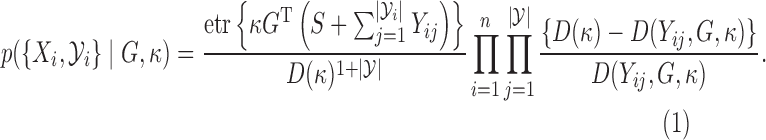
  , so that the joint probability is
 |
(1) |
This procedure recovers samples from  , so that (1) has the correct marginal distribution over
  (Robert & Casella, 2005, p. 51). Later, we will need to sample the rejected variables
  given an observation
  drawn from
  . Simulating from
  involves the two steps in Algorithm 1, which relies on Proposition 1 about
  ; see the Appendix.
Algorithm 1 —
Algorithm to sample from
Input: A sample
, and the parameter value
.
Output: The set of rejected proposals
preceding
.
Sample
independently from
until a point
is accepted.
Discard
, and treat the preceding rejected proposals as
.

Proposition 1 —
The set of rejected samples
preceding an accepted sample
is independent of
:
.
3. Bayesian inference
3.1. Sampling by introducing rejected proposals
Given observations  , and a prior
  , Bayesian inference typically uses Markov chain Monte Carlo simulation to sample from an intractable posterior
  . Split
  as
as  so that the normalization constant factors as
  , with
  simple to evaluate, and
  intractable. Updating
  with
with  fixed is easy, and there are situations where we can place a conjugate prior on
  . Inference for
  is a doubly-intractable problem.
We assume that  has an associated rejection sampling algorithm with proposal density
  . For the
  th observation
  , write the preceding set of rejected samples as
  . The joint density of all samples, both rejected and accepted, is
 |
This involves no intractable terms, so standard techniques can be applied to update  . To introduce the rejected proposals
  , we simply follow Algorithm 1: draw proposals from
  until we have
  acceptances, with the
  th batch of rejected proposals forming the set
  .
.
The ability to produce conditionally independent draws of  is important when, for instance, there exists a conjugate prior
  on
on  for the likelihood
  . Introducing the rejected proposals
  breaks this conjugacy, and the resulting complications in updating
  can slow down mixing, especially when
  is high-dimensional. A much cleaner solution is to sample
  from its conditional posterior
  , introducing the auxiliary variables only when needed to update
  . After updating
  , they can be discarded. Algorithm 2 describes this.
Algorithm 2 —
An iteration of the Markov chain for posterior inference for
Input: The observations
, and the current parameter values
.
Output: New parameter values
.
Run Algorithm 1
times, keeping all the rejected proposals
.
Update
to
with a Markov kernel having
as stationary distribution.
Discard the rejected proposals
.
Sample a new value of
from the conditional
.
3.2. Related work
One of the simplest and most widely applicable Markov chain Monte Carlo algorithms for doubly-intractable distributions is the exchange sampler of Murray et al. (2006). Simplifying an earlier idea by Møller et al. (2006), this algorithm effectively amounts to the following: given the current parameter  , propose a new parameter
  according to some proposal distribution. Additionally, generate a dataset of
  pseudo-observations
  from
from  . The exchange algorithm then proposes to exchange parameters associated with datasets. Murray et al. (2006) show that all intractable terms cancel out in the resulting acceptance probability, and that the resulting Markov chain has the correct stationary distribution.
While the exchange algorithm is applicable whenever one can sample from the likelihood  , it does not exploit the mechanism used to produce these samples. When the latter is a rejection sampling algorithm, each pseudo-observation is preceded by a sequence of rejected proposals. These are all discarded, and only the accepted proposals are used to evaluate the new parameter
  . By contrast our algorithm explicitly instantiates these rejected proposals, so that they can be used to make good proposals. In our experiments, we use a Hamiltonian Monte Carlo sampler on the augmented space and exploit gradient information to make nonlocal moves with a high probability of acceptance. For reasonable acceptance probabilities under the exchange sampler, one must make local updates to
  , or resort to complicated annealing schemes. Of course, the exchange sampler is applicable when no efficient rejection sampling scheme exists, such as when carrying out parameter inference for a Markov random field.
Another framework for doubly-intractable distributions is the pseudo-marginal approach of Andrieu & Roberts (2009). The idea here is that even if we cannot exactly evaluate the acceptance probability, it is sufficient to use a positive, unbiased estimator: this will still result in a Markov chain with the correct stationary distribution. In our case, instead of requiring an unbiased estimate, we bound  by choosing
  . Additionally, like the exchange sampler, the pseudo-marginal method provides a mechanism to evaluate a proposed
  ; making good proposals (Dahlin et al., 2015) is less obvious. Other papers are Beskos et al. (2006), based on a rejection sampling algorithm for diffusions, and Walker (2011).
Most closely related to our ideas is a sampler from Adams et al. (2009); see also §7. Their problem also involved inferences on the parameters governing the output of a rejection sampling algorithm. Like us, they augment the state space to include the rejected proposals  , and like us, given these auxiliary variables, they use Hamiltonian Monte Carlo to efficiently update parameters. However, rather than generating independent realizations of
  when needed, Adams et al. (2009) outlined a set of Markov transition operators to perturb the current configuration of
  , while maintaining the correct stationary distribution. With prespecified probabilities, they proposed adding a new variable to
  , deleting a variable from
  and perturbing the value of an existing element in
  . These local updates to
  can slow down Markov chain mixing, require the user to specify a number of parameters, and also involve calculating Metropolis–Hastings acceptance probabilities for each local step. Furthermore, the Markov nature of their updates require them to maintain the rejected proposals at all times; this can break any conjugacy, and complicate inference for other parameters.
4. Convergence properties
Write the Markov transition density of our chain as  , and the
  -fold transition density as
  . The Markov chain is uniformly ergodic if constants
  and
and  exist such that for all
  and
and  ,
,  The term to the left is twice the total variation distance between the desired posterior and the state of the Markov chain initialized at
  after
after  iterations. Small values of
  imply faster mixing. The following minorization condition is sufficient for uniform ergodicity (Jones & Hobert, 2001): there exists a probability density
  and a
and a  such that for all
  ,
,
 |
(2) |
When this holds, the mixing rate  , so that a large
  implies rapid mixing.
Our Markov transition density first introduces the rejected proposals  , and then conditionally updates
  . The set
  preceding the
  th observation takes values in the union space
  . The output of the rejection sampler, including the
  th observation, lies in the product space
  with density given by equation (1), so that any
  has probability
 |
(3) |
Here,  is the measure with respect to which the densities
  and
and  are defined, and it is easy to see that equation (3) integrates to 1. From Bayes' rule, the conditional density over
  is
is
 |
(4) |
The fact that the right-hand side does not depend on  is another proof of Proposition 1. Equation (4) also motivates the use of our algorithm outside the context of rejection sampling: we can view
  as convenient auxiliary variables that are independent of
  , and whose density is such that
  cancels when evaluating the joint density of
  .
.
The density from equation (4) characterizes the data augmentation step of our sampling algorithm. In practice, we need as many draws from this density as there are observations. The next step involves updating  given
given  , and depends on the problem at hand. We simplify matters by assuming that we can sample from
  independently of the old
  : this is the classical data augmentation algorithm. We also assume that the functions
  and
and  are uniformly bounded from above and below by finite, positive quantities
  and
and  respectively, and that
  . It follows that there exist positive numbers
  and
and  that minimize
  and
and  . We can now state our result.
Theorem 1 —
Assume that
and that positive bounds
exist with
and
as defined earlier. Further assume we can sample from the conditional
. Then our data augmentation algorithm is uniformly ergodic with mixing rate
bounded above by
, where
and
is the number of observations.
Despite our assumptions, our theorem has a number of useful implications. The ratio  is a measure of how flat the function
  is, and the closer it is to unity, the more efficient rejection sampling for
  can be. From our result, the smaller the ratio, the larger the bound on
  , suggesting slower mixing. This is consistent with more rejected proposals
  increasing the coupling between successive
  s in the Markov chain. On the other hand, a small
  suggests a proposal distribution tailored to
  , and our result shows that this implies faster mixing. The numbers
  and
and  are measures of mismatch between the target and proposal density, with small values giving better mixing. Finally, more observations
  result in slower mixing. We suspect that this last property holds for most exact samplers for doubly-intractable distributions, though we are unaware of any such result.
Even without assuming we can sample from  , our ability to sample
  independently means that the marginal chain over
  is Markovian. By contrast, existing approaches (Adams et al., 2009; Walker, 2011) only produce dependent updates in the complicated auxiliary space: they sample from
  by making local updates to
  . Consequently, these chains are Markovian only in the complicated augmented space, and the marginal processes over
  have long-term dependencies. Besides affecting mixing, this can also complicate analysis.
5. Flow cytometry data
We apply our algorithm to a dataset of flow cytometry measurements from patients subjected to bone-marrow transplant (Brinkman et al., 2007). This graft-versus-host disease dataset has 6809 control and 9083 positive observations, corresponding to whether donor immune cells attack host cells. Each observation consists of four biomarker measurements truncated between 0 and 1024, though more complicated truncation rules are often used according to operator judgement (Lee & Scott, 2012). We normalize and plot the first two dimensions, markers CD4 and CD8b, in Fig. 1. Truncation complicates the clustering of observations into homogeneous groups, an important step in the flow-cytometry pipeline called gating. Consequently, Lee & Scott (2012) propose an expectation-maximization algorithm for truncated Gaussian mixture models, which must be adapted if different mixture components or truncation rules are used.
Fig. 1.

Scatterplots of the first two dimensions for the control (left) and positive (right) group. Contours represent log posterior-mean densities under a Dirichlet process mixture.
We model the untruncated distribution for each group as a Dirichlet process mixture of Gaussian kernels (Lo, 1984), with points outside the four-dimensional unit hypercube discarded to form the normalized dataset. The Dirichlet process mixture model is a flexible nonparametric prior over densities parameterized by a concentration parameter  and a base probability measure. We set
  , and for the base measure, which gives the distribution over cluster parameters, we use a normal-inverse-Wishart distribution. Given the rejected variables, we can use standard techniques to update a representation of the Dirichlet process. We follow the blocked-sampler of Ishwaran & James (2001) based on the stick-breaking representation of the Dirichlet process, using a truncation level of 50 clusters. This corresponds to updating
  , step 2 in Algorithm 2. Having done this, we discard the old rejected samples, and produce a new set by drawing from a 50-component Gaussian mixture model, corresponding to step 1 in Algorithm 2.
Figure 1 shows the log mean posterior densities for the first two dimensions from 10 000 iterations. While the control group has three clear modes, these are much less pronounced in the positive group. Directly modelling observations with a Gaussian mixture model obscured this by forcing modes away from the edges. One can use components with bounded support in the mixture model, such as a Dirichlet process mixture of Beta densities; however, these do not reflect the underlying data generation process, and are unsuitable when different groups have different truncation levels. By contrast, it is easy to extend our modelling ideas to allow groups to share components, allowing better identification of disease predictors.
Our sampler took less than two minutes to run 1000 iterations, not much longer than a typical Dirichlet process sampler for datasets of this size. The average number of augmented points was 3960 and 4608 for the two groups. We study our sampler more systematically in the next section, but this application demonstrates the flexibility and simplicity of our main idea.
6. Bayesian inference for the matrix Langevin distribution
6.1. The matrix Langevin distribution on the Stiefel manifold
The Stiefel manifold  is the space of all
  orthonormal matrices, that is,
  matrices
  such that
  , where
  is the
  identity matrix. When
  , this is the
  hypersphere
  , and when
  , this is the space of all orthonormal matrices
  . Probability distributions on the Stiefel manifold play an important role in statistics, signal processing and machine learning, with applications ranging from studies of orientations of orbits of comets and asteroids to principal components analysis to the estimation of rotation matrices. The simplest such distribution is the matrix Langevin distribution, an exponential-family distribution whose density with respect to the invariant Haar volume measure (Edelman et al., 1998) is
  . Here
  is the exponential-trace, and
  is a
is a  matrix. The normalization constant
  is the hypergeometric function with matrix arguments, evaluated at
  (Chikuse, 2003). Let
  be the singular value decomposition of
  , where
  and
and  are
are  and
and  orthonormal matrices, and
  is a positive diagonal matrix. We parameterize
  by
by  , and one can think of
  and
and  as orientations, with
  controlling the concentration in directions determined by these orientations. Large values of
  imply concentration along the associated directions, while setting
  to zero gives the uniform distribution on the Stiefel manifold. It can be shown (Khatri & Mardia, 1977) that
  , so that this depends only on
  . We write it as
  ). In our Bayesian analysis, we place independent priors on
  and
and  . The last two lie on the Stiefel manifolds
  and
and  , and we place matrix Langevin priors
  and
and  on these: we will see below that these are conditionally conjugate. We place independent Gamma priors on the diagonal elements of
  . However, the difficulty in evaluating the normalization constant
  makes posterior inference for
  doubly intractable. Thus, in a 2006 University of Iowa PhD thesis, Camano-Garcia keeps
  constant, while Hoff (2009a) uses a first-order Taylor expansion of the intractable term to run an approximate sampling algorithm. Below, we show how fully Bayesian inference can be carried out for this quantity as well.
6.2. A rejection sampling algorithm
We first describe a rejection sampling algorithm from Hoff (2009b) to sample from  . For simplicity, assume
  is the identity matrix. In the general case, we simply rotate the resulting draw by
  , since if
  , then
  . At a high level, the algorithm sequentially proposes vectors from the matrix Langevin on the unit sphere: this is also called the von Mises–Fisher distribution and is easy to simulate (Wood, 1994). The mean of the
  th vector is column
  of
of  ,
,  , projected onto the nullspace of the earlier vectors,
  . This sampled vector is then projected back onto
  and normalized, and the process is repeated
  times. Call the resulting distribution
  ; for more details, see Algorithm 3 and Hoff (2009b).
Algorithm 3 —
Proposal
for the matrix Langevin distribution (Hoff, 2009b)
Input: Parameters
; write
for column
of
, and
for element
of
.
Output: An output
; write
for column
of
.
Sample
.
For
Construct
, an orthogonal basis for the nullspace of
.
Sample
.
Set
Letting  be the modified Bessel function of the first kind,
  is a density on the Stiefel manifold with
 |
Write  for the reciprocal of the term in braces. Since
  is an increasing function of
  , and
, and  , we have the following bound
  for
for  :
:
 |
This implies that  , allowing the following rejection sampler: sample
  from
from  , and accept with probability
  . The accepted proposals come from
  , and for samples from
  , post multiply these by
  .
.
6.3. Posterior sampling
Given a set of  observations
  , and writing
  , we have:
 |
At a high level, our approach is a Gibbs sampler that sequentially updates  and
and  . The pair of matrices
  correspond to the tractable
  in Algorithm 2, while
  corresponds to
  . Updating the first two is straightforward, while the third requires our augmentation scheme.
- Updating
 and
and  : With a matrix Langevin prior on
  , the posterior is
This is just the matrix Langevin distribution over rotation matrices, and one can sample from this following §6.2. From here onwards, we will rotate the observations by
 , allowing us to ignore this term. Redefining
  as
as  , the posterior over
  is also matrix Langevin,

- Updating
 : Here, we exploit the rejection sampler scheme of the previous section, and instantiate the rejected proposals using Algorithm 1. From §6.2, the joint probability is
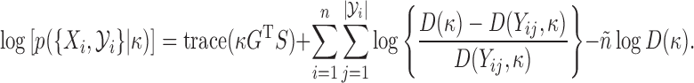
(5)
All terms in (5) can be evaluated easily, allowing a simple Metropolis–Hastings algorithm in this augmented space. In fact, we can calculate gradients to run a Hamiltonian Monte Carlo algorithm (Neal, 2010) that makes significantly more efficient proposals than a random-walk sampling algorithm. In particular, let  , and
, and  . The log joint probability
  is
is
 |
In the Appendix, we give an expression for the gradient of this loglikelihood. We use this to construct a Hamiltonian Monte Carlo sampler (Neal, 2010) for  . Here, it suffices to note that a proposal involves taking
  leapfrog steps of size
  along the gradient, and accepting the resulting state with probability proportional to the product of equation (5), and a simple Gaussian momentum term. The acceptance probability depends on how well the
  -discretization approximates the continuous dynamics of the system, and choosing a small
  and a large
  can give global moves with high acceptance probability. A large
  however costs a large number of gradient evaluations. We study this trade-off in §6.5.
6.4. Vectorcardiogram dataset
The vectorcardiogram is a loop traced by the cardiac vector during a cycle of the heart beat. The two directions of orientation of this loop in three dimensions form a point on the Stiefel manifold. The dataset of Downs et al. (1971) includes 98 such recordings, and is displayed in Fig. 2(a). We represent each observation with a pair of orthonormal vectors, with the cone of lines to the right forming the first component. This empirical distribution possesses a single mode, so that the matrix Langevin distribution seems a suitable model.
Fig. 2.

(a) Vector cardiogram dataset with inferences. Bold solid lines are maximum likelihood estimates of  , and solid circles contain
  posterior mass. Dashed circles are
  predictive probability regions. (b) Posterior distribution over
  and
and  , circles are maximum likelihood estimates.
We place independent exponential priors with mean 10 and variance 100 on the scale parameter  , and a uniform prior on the location parameter
  . We restrict
  to be the identity matrix. Inferences were carried out using the Hamiltonian sampler to produce 10 000 samples, with a burn-in period of 1000. For the leapfrog dynamics, we set a step size of 0
 3, with the number of steps equal to 5. We fix the mass parameter to the identity matrix. We implemented all algorithms in R (R Development Core Team, 2016), building on the rstiefel package of Hoff (2009b). Simulations were run on an Intel Core 2 Duo 3 Ghz CPU. For comparison, we include the maximum likelihood estimates of
  and
and  . For
. For  and
and  , these were 11
 9 and 5
 9, and we plot these in Fig. 2(b) as circles.
The bold straight lines in Fig. 2(a) show the maximum likelihood estimates of the components of  , with the small circles corresponding to
  Bayesian credible regions estimated from the Monte Carlo output. The dashed circles correspond to
  predictive probability regions for the Bayesian model. For these, we generated 50 points on
  for each sample, with parameters specified by that sample. The dashed circles contain
  of these points across all samples. Figure 2(b) shows the posterior over
  and
and  .
.
6.5. Comparison of exact samplers
To quantify sampler efficiency, we estimate the effective sample sizes produced per unit time. This corrects for correlation between successive Markov chain samples by estimating the number of independent samples produced; for this we used the rcoda package of Plummer et al. (2006).
Figure 3(a) shows the effective sample size per second for two Metropolis–Hastings samplers, the exchange sampler and our latent variable sampler on the vectorcardiogram dataset. Both perform a random walk in the  -space, with the steps drawn for a normal distribution whose variance increases along the horizontal axis. The figure shows that both samplers' performance peaks when the proposals have a variance between 1 and
  , with the exchange sampler performing slightly better. However, the real advantage of our sampler is that introducing the latent variables results in a joint distribution with no intractable terms, allowing the use of more sophisticated sampling algorithms. Figure 3(b) studies the Hamiltonian Monte Carlo sampler described at the end of §3.1. Here we vary the size of the leapfrog steps along the horizontal axis, with the different curves corresponding to different numbers of such steps. This performs an order of magnitude better than either of the previous algorithms, with performance peaking with 3 to 5 steps of size 0
 3 to 0
 5, fairly typical values for this algorithm. This shows the advantage of exploiting gradient information in exploring the parameter space.
Fig. 3.

Effective samples per second for (a) random walk and (b) Hamiltonian samplers. From bottom to top at abscissa 0 5: (a) Metropolis–Hastings data-augmentation sampler and exchange sampler, and (b) 1, 10, 5 and 3 leapfrog steps of the Hamiltonian sampler.
6.6. Comparison with an approximate sampler
In this section, we consider an approximate sampler based on an asymptotic approximation to  for large values of
  (Khatri & Mardia, 1977):
 |
We use this approximation in the acceptance probability of a Metropolis–Hastings algorithm; it can similarly be used to construct a Hamiltonian sampler. For a more complicated but accurate approximation, see Kume et al. (2013). In general however, using such approximate schemes involves the ratio of two approximations, and can have very unpredictable performance.
On the vectorcardiogram dataset, the approximate sampler is about forty times faster than the exact samplers. For larger datasets, this difference will be even greater, and the real question is how accurate the approximation is. Our exact sampler allows us to study this: we consider the Stiefel manifold  , with the three diagonal elements of
  set to
  and 10. With this setting of
  , and a random
  , we generate datasets with 50 observations, with
  taking values
  and 10. In each case, we estimate the posterior mean of
  by running the exchange sampler, and treat this as the truth. We compare this with posterior means returned by our Hamiltonian sampler, as well as the approximate sampler. Figure 4 shows these results. As expected, the two exact samplers agree, and the Hamiltonian sampler has almost no error. For values of
  around 5, the estimated posterior mean for the approximate sampler is close to that of the exact samplers. Smaller values lead to an approximate posterior mean that underestimates the actual posterior mean, while in higher dimensions, the opposite occurs. Recalling that
  controls the concentration of the matrix Langevin distribution about its mode, this implies that in high dimensions, the approximate sampler underestimates uncertainty in the distribution of future observations.
Fig. 4.

Errors in the posterior mean for the vectorcardiogram dataset. Each panel is a different component of  ; solid/dashed lines are the Hamiltonian/approximate sampler.
7. The Gaussian process density sampler
7.1. Nonparametric density modelling with a transformed Gaussian process
Our next application is the Gaussian process density sampler of Adams et al. (2009), a nonparametric prior for probability densities induced by a logistic transformation of a random function from a Gaussian process. Letting  denote the logistic function, the random density is
 |
with  a parametric base density and
  denoting a Gaussian process. The inequality
  allows a rejection sampling algorithm by making proposals from
  . At a proposed location
  , we sample the function value
  conditioning on all previous evaluations, and accept the proposal with probability
  . Such a scheme involves no approximation error, and only requires evaluating the random function on a finite set of points. Algorithm 4 describes the steps involved in generating
  observations.
Algorithm 4 —
Generate
new samples from the Gaussian process density sampler
Input: A base probability density
.
Previous accepted and rejected proposals
and
.
Gaussian process evaluations
and
at these locations.
Output:
new samples
, with the associated rejected proposals
.
Gaussian process evaluations
and
at these locations.
Repeat
Sample a proposal
from
.
Sample
, the Gaussian process evaluated at
, conditioning on
,
,
and
.
With probability
Accept
and add it to
. Add
to
.
Else
Reject
and add it to
. Add
to
.
Until
samples are accepted.

7.2. Posterior inference
Given observations  , we are interested in
  , the posterior over the underlying density. Since
  is determined by the modulating function
  , we focus on
  . While this quantity is doubly intractable, after augmenting the state space to include the proposals
  from the rejection sampling algorithm,
  has density
  with respect to the Gaussian process prior; see also Adams et al. (2009). In words, the posterior over
  evaluated at
  is just the posterior from a Gaussian process classification problem with a logistic link-function, and with the accepted and rejected proposals corresponding to the two classes. Markov chain Monte Carlo methods such as Hamiltonian Monte Carlo or elliptical slice sampling (Murray et al., 2010) are applicable in such a situation. Given
  on
on  , the Gaussian process can be evaluated anywhere else by conditionally sampling from a multivariate normal.
Sampling the rejected proposals  given
given  and
and  is straightforward using Algorithm 1: run the rejection sampler until
  accepts, and treat the rejected proposals generated along the way as
  . In practice, we do not have access to the entire function
  , only its values evaluated on
  and
and  , the locations of the previous thinned variables. However, just as under the generative mechanism, we can retrospectively evaluate the function
  where needed. After proposing from
  , we sample the value of the function at this location conditioned on all previous evaluations, and use this value to decide whether to accept or reject. We outline the inference algorithm in Algorithm 5, noting that it is much simpler than that proposed in Adams et al. (2009). We also refer to that paper for limitations of the exchange sampler in this problem.
Algorithm 5 —
A Markov chain iteration for inference in the Gaussian process density sampler
Input: Observations
with corresponding function evaluations
.
Current rejected proposals
with corresponding function evaluations
.
Output: New rejected proposals
.
New Gaussian process evaluations
and
at
and
.
New hyperparameters.
Run Algorithm 4 to produce
accepted samples, with
and
as inputs.
Replace
and
with values returned by the previous step; call these
and
.
Update
and
using for example, hybrid Monte Carlo, to get
and
.
Update Gaussian process and base-distribution hyperparameters.
7.3. Experiments
Voice changes are a symptom and measure of the onset of Parkinson's disease, and one attribute is voice shimmer, a measure of variation in amplitude. We consider a dataset of such measurements for subjects with and without the disease (Little et al., 2007), with 147 measurements with, and 48 without the disease. We normalized these to vary from 0 to 5, and used the model of Adams et al. (2009) as a prior on the underlying probability densities. We set  to a normal
  , with a normal-inverse-Gamma prior on
  . The latter had its mean, inverse-scale, degrees-of-freedom and variance set to 0,
 1,1 and 10. The Gaussian process had a squared-exponential kernel, with variance and length-scale of 1. For each case, we ran a Matlab implementation of our data augmentation algorithm to produce 2000 posterior samples after a burn-in of 500 samples.
Figure 5(a) shows the resulting posterior over densities, corresponding to  in Algorithm 2. The control group is fairly Gaussian, while the disease group is skewed to the right. Figure 5(b) focuses on the deviation from normality by plotting the posterior over the latent function
  . We see that to the right of 0
 5, this deviation is larger than its prior mean of zero, implying larger probability than under a Gaussian density. Figure 6 studies the distribution of the rejected proposals
  . Figure 6(a) shows the distribution of their locations: most of these occured near the origin. Here, the disease density reverts to Gaussian or even sub-Gaussian density, with the intensity function taking small values. Figure 6(b) is a histogram of the number of rejected proposals: this is typically around 100 to 150, though the largest value we observed was 668. Since inference on the latent function involves evaluating it at the accepted as well as rejected proposals, the largest covariance matrix we had to deal with was about
  ; typical values were around
  . Using the same set-up as §6.5, it took a naïve Matlab implementation 26 and 18 minutes to run 2500 iterations for the disease and control datasets. One can imagine computations becoming unwieldy for a large number of observations, or when there is large mismatch between the true density and the base-measure
  . In such situations, one might have to choose the Gaussian process covariance kernel more carefully, use one of many sparse approximation techniques, or use other nonparametric priors like splines instead. In all these cases, we can use our algorithm to recover the rejected proposals
  , and given these, posterior inference for
  can be carried out using standard techniques.
Fig. 5.

Inferences for the Parkinson's dataset: (a) posterior density for positive (solid) and control (dashed) groups, (b) posterior distribution of the Gaussian process function for positive group with observations. Both panels show the median with 80 percent credible intervals.
Fig. 6.

Rejected proposals for the Parkinson's dataset: (a) kernel density estimate of locations of rejected proposals, and (b) histogram of the number of rejected proposals for the positive group.
8. Future work
Our algorithm, while exact, also provides a framework for faster, approximate algorithms. A priori, the number of rejected proposals preceeding any observation is unbounded: one can bound the computational cost of an iteration by limiting the maximum number of rejected proposals. Similarly, one might share rejected proposals across observations. We leave the study of such approximate sampling algorithms for future research. Also left open is a more careful analysis of Markov mixing rates for the applications we considered. There are also a number of applications that we have not described here: particularly relevant are rejection samplers for diffusions (Beskos et al., 2006; Bladt & Sørensen, 2014).
Acknowledgement
This work was supported by the National Institute of Environmental Health Sciences of the National Institutes of Health. We are grateful to the editor and reviewers for valuable comments.
Appendix
Proofs
Proof of Proposition 1 —
Rejection sampling first proposes from
, and then accepts with probability
. Conceptually, one can first decide whether to accept or reject, and then conditionally sample the location. The marginal acceptance probability is
, the area under
divided by that under
. An accepted sample
is distributed as the target distribution
, while rejected samples are distributed as
. This two-component mixture is just the proposal
. While this mixture representation loses the computational benefits of the original algorithm, it shows that the location of an accepted sample is independent of the past, and consequently, that the number and locations of rejected samples preceding an accepted sample is independent of the location of that sample. Thus, one can use the rejected samples preceding any other accepted sample.
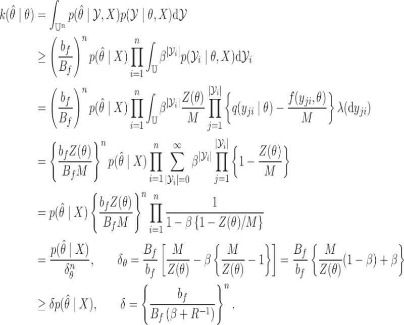
Proof of Theorem 1 —
It follows from Bayes' rule and the assumed bounds that for an observation
,
Let the number of observations
be
. Then,
Thus
satisfies equation (2), with
, and
.
Gradient information
For  pairs
pairs  , with
  , and
, and  , we have
 |
Let  , and
, and  . Since
  ,
,
 |
Then, writing  , and
, and  for
for  , we have
 |
References
- Aban I. B., Meerschaert M. M. & Panorska A. K. (2006). Parameter estimation for the truncated Pareto distribution. J. Am. Statist. Assoc. 101, 270–7. [Google Scholar]
- Adams R. P., Murray I. & MacKay D. J. C. (2009). The Gaussian process density sampler. In Adv. Neural Info. Process. Syst.21, D. Koller, D. Schuurmans, Y. Bengio & L. Bottou, eds. Cambridge, MA: MIT Press, pp. 9–16.
- Alai D. H., Landsman Z. & Sherris M. (2013). Lifetime dependence modelling using a truncated multivariate Gamma distribution. Insurance Math. Econom. 52, 542–9. [Google Scholar]
- Andrieu C. & Roberts G. O. (2009). The pseudo-marginal approach for efficient Monte Carlo computations. Ann. Statist. 37, 697–725. [Google Scholar]
- Beskos A., Papaspiliopoulos O., Roberts G. O. & Fearnhead P. (2006). Exact and computationally efficient likelihood-based estimation for discretely observed diffusion processes. J. R. Statist. Soc. B 68, 333–82. [Google Scholar]
- Bladt M. & Sørensen M. (2014). Simple simulation of diffusion bridges with application to likelihood inference for diffusions. Bernoulli 20, 645–75. [Google Scholar]
- Brinkman R. R., Gasparetto M., Lee S.-J. J., Ribickas A. J., Perkins J., Janssen W., Smiley R. & Smith C. (2007). High-content flow cytometry and temporal data analysis for defining a cellular signature of graft-versus-host disease. Biol. Blood Marrow Trans. 13, 691–700. [DOI] [PMC free article] [PubMed] [Google Scholar]
- Chikuse Y. (2003) Statistics on Special Manifolds. New York: Springer. [Google Scholar]
- Dahlin J., Lindsten F. & Schön T. B. (2015). Particle Metropolis–Hastings using gradient and Hessian information. Statist Comp. 25, 81–92. [Google Scholar]
- Downs T. D., Liebman J. & Mackay W. (1971). Statistical methods for vectorcardiogram orientations. In Vectorcardiography2: Proc. XIth Intn. Symp. Vectorcardiography, R. H. I. Hoffman & E. E. Glassman, eds. Amsterdam: North-Holland, pp. 216–22.
- Edelman A., Arias T. A. & Smith S. T. (1998). The geometry of algorithms with orthogonality constraints. SIAM J. Matrix Anal. Appl. 20, 303–53. [Google Scholar]
- Goethals K., Ampe B., Berkvens D., Laevens H., Janssen P. & Duchateau L. (2009). Modeling interval-censored, clustered cow udder quarter infection times through the shared gamma frailty model. J. Agric. Biol. Envir. Statist. 14, 1–14. [Google Scholar]
- Hoff P. D. (2009a). A hierarchical eigenmodel for pooled covariance estimation. J. R. Statist. Soc. B 71, 971–92. [Google Scholar]
- Hoff P. D. (2009b). Simulation of the matrix Bingham–von Mises–Fisher distribution, with applications to multivariate and relational data. J. Comp. Graph. Statist. 18, 438–56. [Google Scholar]
- Ishwaran H. & James L. F. (2001). Gibbs sampling methods for stick-breaking priors. J. Am. Statist. Assoc. 96, 161–73. [Google Scholar]
- Jones G. L. & Hobert J. P. (2001). Honest exploration of intractable probability distributions via Markov chain Monte Carlo. Statist. Sci. 16, 312–34. [Google Scholar]
- Khatri C. G. & Mardia K. V. (1977). The von Mises–Fisher matrix distribution in orientation statistics. J. R. Statist. Soc. B 39, 95–106. [Google Scholar]
- Kume A., Preston S. P. & Wood A. T. A. (2013). Saddlepoint approximations for the normalizing constant of Fisher–Bingham distributions on products of spheres and Stiefel manifolds. Biometrika 100, 971–84. [Google Scholar]
- Lee G. & Scott C. (2012). EM algorithms for multivariate Gaussian mixture models with truncated and censored data. Comput. Statist. Data Anal. 56, 2816–29. [Google Scholar]
- Liechty M. W., Liechty J. C. & Müller P. (2009). The shadow prior. J. Comp. Graph. Statist. 18, 368–83. [Google Scholar]
- Little M. A., McSharry P. E., Roberts S. J., Costello D. A. E. & Moroz I. M. (2007). Exploiting nonlinear recurrence and fractal scaling properties for voice disorder detection. Biomed. Eng. Online, 6, 23. [DOI] [PMC free article] [PubMed] [Google Scholar]
- Lo A. (1984). On a class of Bayesian nonparametric estimates: I. Density estimates. Ann. Statist. 12, 351–7. [Google Scholar]
- Møller J., Pettitt A. N., Reeves R. & Berthelsen K. K. (2006). An efficient Markov chain Monte Carlo method for distributions with intractable normalising constants. Biometrika 93, 451–8. [Google Scholar]
- Murray I., Ghahramani Z. & MacKay D. J. C. (2006). MCMC for doubly-intractable distributions. In Proc. 22nd Conf. Uncert. Artif. Intell. AUAI Press, pp. 359–66.
- Murray I., Adams R. P. & MacKay D. J. (2010). Elliptical slice sampling. J. Mach. Learn. Res. 9, 541–8. [Google Scholar]
- Neal R. M. (2010). MCMC using Hamiltonian dynamics. In Handbook of Markov Chain Monte Carlo, S. P. Brooks, A. Gelman, G. L. Jones, & X.-L. Meng, eds. Boca Raton, Florida: Chapman & Hall/CRC Press, pp. 113–62.
- Plummer M., Best N., Cowles K. & Vines K. (2006). CODA: Convergence diagnosis and output analysis for MCMC. R News 6, 7–11. [Google Scholar]
- Robert C. P. & Casella G. (2005). Monte Carlo Statistical Methods. New York: Springer, 2nd ed. [Google Scholar]
- R Development Core Team (2016). R: A Language and Environment for Statistical Computing. R Foundation for Statistical Computing, Vienna, Austria. ISBN 3-900051-07-0. http://www.R-project.org.
- Walker S. G. (2011). Posterior sampling when the normalizing constant is unknown. Commun. Statist. B 40, 784–92. [Google Scholar]
- Wood A. T. A. (1994). Simulation of the von Mises–Fisher distribution. Commun. Statist. B 23, 157–64. [Google Scholar]