

Abstract
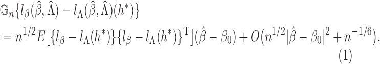
Interval censoring arises frequently in clinical, epidemiological, financial and sociological studies, where the event or failure of interest is known only to occur within an interval induced by periodic monitoring. We formulate the effects of potentially time-dependent covariates on the interval-censored failure time through a broad class of semiparametric transformation models that encompasses proportional hazards and proportional odds models. We consider nonparametric maximum likelihood estimation for this class of models with an arbitrary number of monitoring times for each subject. We devise an EM-type algorithm that converges stably, even in the presence of time-dependent covariates, and show that the estimators for the regression parameters are consistent, asymptotically normal, and asymptotically efficient with an easily estimated covariance matrix. Finally, we demonstrate the performance of our procedures through simulation studies and application to an HIV/AIDS study conducted in Thailand.
Keywords: Current-status data, EM algorithm, Interval censoring, Linear transformation model, Nonparametric likelihood, Proportional hazards, Proportional odds, Semiparametric efficiency, Time-dependent covariate
1. Introduction
Interval-censored data arise when the event or failure of interest is known only to occur within a time interval. Such data are commonly encountered in disease research, where the ascertainment of an asymptomatic event is costly or invasive and so can take place only at a small number of monitoring times. For example, in HIV/AIDS studies, blood samples are periodically drawn from at-risk subjects to look for evidence of HIV sero-conversion. Likewise, biopsies are performed on patients at clinic visits to determine the occurrence or recurrence of cancer.
There are several types of interval-censored data. The simplest and most studied type is
called case-1 or current-status data, which involves only one monitoring time per subject
and is routinely found in cross-sectional studies. When there are two or
 monitoring times per subject, the resulting data are
referred to as case-2 or case-
monitoring times per subject, the resulting data are
referred to as case-2 or case- interval censoring (Huang & Wellner, 1997). The most general and common type allows
for varying numbers of monitoring times among subjects and is termed mixed-case interval
censoring (Schick & Yu, 2000).
interval censoring (Huang & Wellner, 1997). The most general and common type allows
for varying numbers of monitoring times among subjects and is termed mixed-case interval
censoring (Schick & Yu, 2000).
The fact that the failure time is never observed exactly poses theoretical and
computational challenges in semiparametric regression analysis of such data. Huang (1995, 1996) and Huang & Wellner (1997)
studied nonparametric maximum likelihood estimation for the proportional hazards and
proportional odds models with case-1 and case-2 data. The estimators are obtained by the
iterative convex minorant algorithm, which becomes unstable for large datasets. Sieve
maximum likelihood estimation for the proportional odds model was considered by Rossini & Tsiatis (1996) with case-1 data and
by Huang & Rossini (1997) and Shen (1998) with case-2 data; however, it is
difficult to choose an appropriate sieve parameter space and, especially, to choose the
number of knots. For the proportional odds model with case-1 and case-2 data, Rabinowitz et al. (2000) derived an approximate
conditional likelihood, which does not perform well in small samples. Gu et al. (2005), Sun &
Sun (2005), Zhang et al. (2005) and
Zhang & Zhao (2013) constructed
rank-based estimators for linear transformation models, but such estimators are
computationally demanding and statistically inefficient. None of the existing work
accommodates time-dependent covariates or can handle case- or mixed-case interval
censoring.
or mixed-case interval
censoring.
In this paper we consider interval censoring in the most general form, that is, mixed-case data. We study nonparametric maximum likelihood estimation for a broad class of transformation models that allows time-dependent covariates and includes the proportional hazards and proportional odds models as special cases. We develop an EM-type algorithm, which is demonstrated to perform satisfactorily in a wide variety of settings, even with time-dependent covariates. Using empirical process theory (van der Vaart & Wellner, 1996; van de Geer, 2000) and semiparametric efficiency theory (Bickel et al., 1993), we establish that, under mild conditions, the proposed estimators for the regression parameters are consistent and asymptotically normal and the limiting covariance matrix attains the semiparametric efficiency bound and can be estimated analytically by the profile likelihood method (Murphy & van der Vaart, 2000). The theoretical development requires careful treatment of the time trajectories of covariate processes and the joint distribution for an arbitrary sequence of monitoring times.
2. Methods
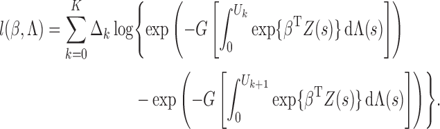
2.1. Transformation models and likelihood construction
Let  denote the failure time, and let
 denote a
  -vector of potentially time-dependent
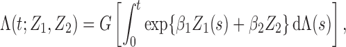
covariates. Under the semiparametric transformation model, the cumulative hazard function
for
-vector of potentially time-dependent
covariates. Under the semiparametric transformation model, the cumulative hazard function
for  conditional on
  takes the
form
takes the
form
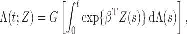 |
(1) |
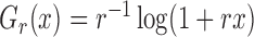
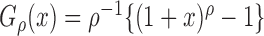
where
 is a specific transformation function that is strictly
increasing and
is a specific transformation function that is strictly
increasing and  is an unknown increasing function (Zeng & Lin, 2006). The choices of
 and
and 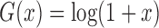 yield the proportional
hazards and proportional odds models, respectively. It is useful to consider the class of
frailty-induced transformations
yield the proportional
hazards and proportional odds models, respectively. It is useful to consider the class of
frailty-induced transformations
 |
where  is the density function of a
frailty variable with support
is the density function of a
frailty variable with support  . The choice of the gamma density with unit
mean and variance
. The choice of the gamma density with unit
mean and variance  for
for  yields the class of logarithmic
transformations,
yields the class of logarithmic
transformations, 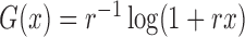
 , and the
choice of the positive stable distribution with parameter
, and the
choice of the positive stable distribution with parameter  yields the
class of Box–Cox transformations,
yields the
class of Box–Cox transformations, 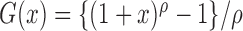 . When
all the covariates are time-independent, model (1) can be rewritten as a linear transformation model
. When
all the covariates are time-independent, model (1) can be rewritten as a linear transformation model
 |
where  is an error
term with distribution function
is an error
term with distribution function 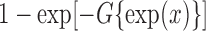 (Chen et al., 2002). Thus,
 can be interpreted as the effects of covariates on a
transformation of
can be interpreted as the effects of covariates on a
transformation of  .
.
We formulate the mixed-case interval censoring by assuming that the number of monitoring
times, denoted by  , is random and that there exists a random sequence of
monitoring times, denoted by
, is random and that there exists a random sequence of
monitoring times, denoted by 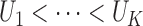 . We do not model
 . Write
 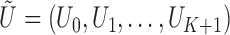 , where
  and
and  .
Also, define
.
Also, define 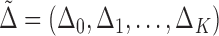 , where
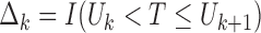
 with
with
 denoting the indicator function. Then the observed data
from a random sample of
denoting the indicator function. Then the observed data
from a random sample of  subjects consist of
 , where
 and
and  . If
. If  or 2
or 2
 , then the observation scheme becomes case-1 or
case-2, respectively.
, then the observation scheme becomes case-1 or
case-2, respectively.
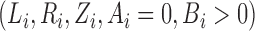
Suppose that  is independent of
  conditional on
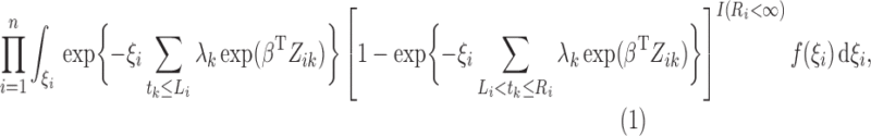
 . Then the observed-data likelihood function concerning
parameters
. Then the observed-data likelihood function concerning
parameters  takes the form
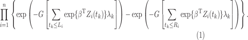
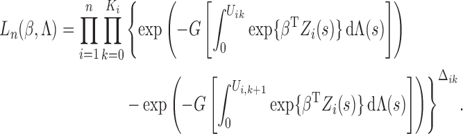 |
Since only one  is unity
for each subject and the others equal zero,
is unity
for each subject and the others equal zero,
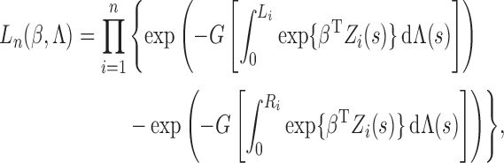 |
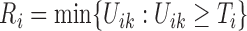
where  is the smallest interval
that brackets
is the smallest interval
that brackets  , i.e.,
 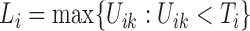 and
and
 . Clearly,
  indicates that
the
indicates that
the  th subject is left censored, while
 indicates that the subject is right censored.
Remark 1. —
The sequence of monitoring times may not be completely observed and, in fact, need not be for the purpose of inference. We only need to know the values of
and
, since the other monitoring times do not contribute to the likelihood. The theoretical development, however, requires consideration of the joint distribution for the entire sequence of monitoring times.
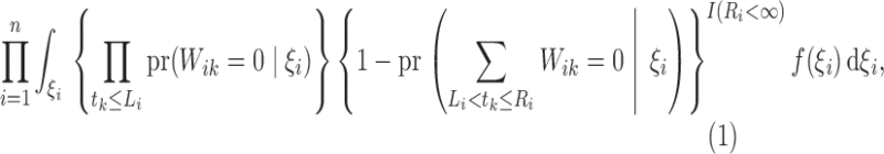
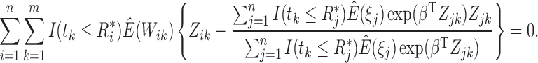
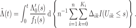
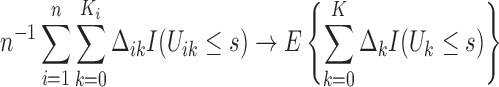
2.2. Nonparametric maximum likelihood estimation
To estimate  and
and  , we adopt the nonparametric
maximum likelihood approach, under which
, we adopt the nonparametric
maximum likelihood approach, under which  is regarded as a step function
with nonnegative jumps at the endpoints of the smallest intervals that bracket the failure
times. Specifically, if
is regarded as a step function
with nonnegative jumps at the endpoints of the smallest intervals that bracket the failure
times. Specifically, if  denotes the set
consisting of 0 and the unique values of
denotes the set
consisting of 0 and the unique values of  and
and 
 , then the estimator for
 is a step function with jump size
 at
at  and with
  . Hence,
we maximize the function
. Hence,
we maximize the function
 |
(2) |
Direct maximization of (2) is difficult due to the lack of an
analytical expression for the parameters 
 . An
even more severe challenge is that not all the
. An
even more severe challenge is that not all the  and
and  are informative
about the failure times, so many of the
are informative
about the failure times, so many of the  are zero and hence lie on
the boundary of the parameter space. For example, if there are no interval endpoints
between some
are zero and hence lie on
the boundary of the parameter space. For example, if there are no interval endpoints
between some  and
and  with
with  , then the
jump size at
, then the
jump size at  must be zero in order to maximize (2). The existing iterative convex minorant
algorithm works only for the proportional hazards and proportional odds models with
time-independent covariates (Huang & Wellner,
1997). In the following, we construct an EM algorithm to maximize (2).
must be zero in order to maximize (2). The existing iterative convex minorant
algorithm works only for the proportional hazards and proportional odds models with
time-independent covariates (Huang & Wellner,
1997). In the following, we construct an EM algorithm to maximize (2).
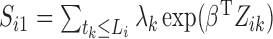
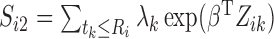
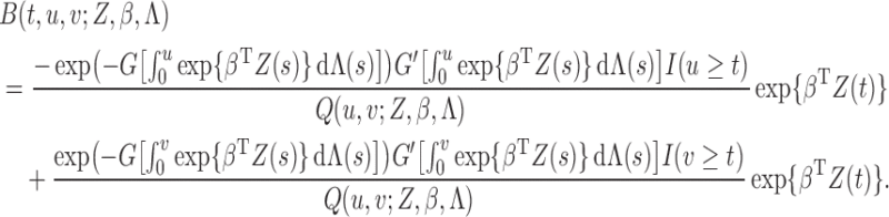
For the class of frailty-induced transformations described in §2.1, the observed-data likelihood can be written as
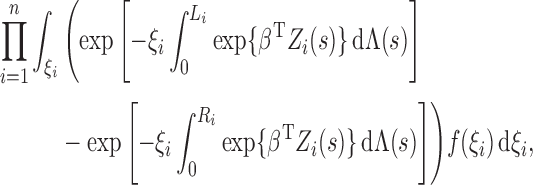 |
so that the estimation of the transformation
model becomes that of the proportional hazards frailty model. With
 as a step function with jumps
  at
at

 , this likelihood
becomes
, this likelihood
becomes
 |
(3) |
where  .
We introduce latent variables
.
We introduce latent variables 
 which, conditional on
  , are independent Poisson random variables with means
 . We show below that the
nonconcave likelihood function given in (3) is equivalent to a likelihood function for these Poisson variables, so the
M-step becomes maximization of a weighted sum of Poisson loglikelihood functions which is
strictly concave and has closed-form solutions for
. We show below that the
nonconcave likelihood function given in (3) is equivalent to a likelihood function for these Poisson variables, so the
M-step becomes maximization of a weighted sum of Poisson loglikelihood functions which is
strictly concave and has closed-form solutions for 
 . Similar Poisson
variables were recently used by Wang et al.
(2015) in spline-based estimation of the proportional hazards model with
time-independent covariates.
. Similar Poisson
variables were recently used by Wang et al.
(2015) in spline-based estimation of the proportional hazards model with
time-independent covariates.
Define 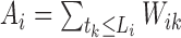 and
and  . Suppose that the observed data consist of
 , where
 means that
  is known to be zero and that
 means that
  is known to be positive, such that
 for
for  and at least one
 for
for 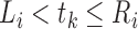 with
with
 . Then the likelihood takes the form
 |
(4) |
which is the same as (3). Thus, maximization of (3) is equivalent to maximum likelihood
estimation based on the data 
 .
.
We maximize (4) through an EM
algorithm by treating  and
and  as missing data. The
complete-data loglikelihood is
as missing data. The
complete-data loglikelihood is
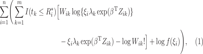 |
(5) |
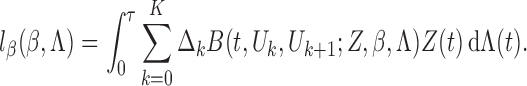
where  . In the M-step, we calculate
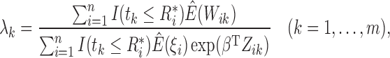 |
(6) |
where  denotes the posterior mean given the observed data. After incorporating (6) into the conditional expectation of
(5), we update
denotes the posterior mean given the observed data. After incorporating (6) into the conditional expectation of
(5), we update
 by solving the following equation using the one-step
Newton–Raphson method:
by solving the following equation using the one-step
Newton–Raphson method:
 |
In the E-step, we evaluate the posterior means  and
and
 . The posterior density function of
 given the observed data is proportional to
 , where
 and
and
 . Hence, we
evaluate the posterior means by noting that for
. Hence, we
evaluate the posterior means by noting that for  ,
,
 |
and for  with
with  ,
,
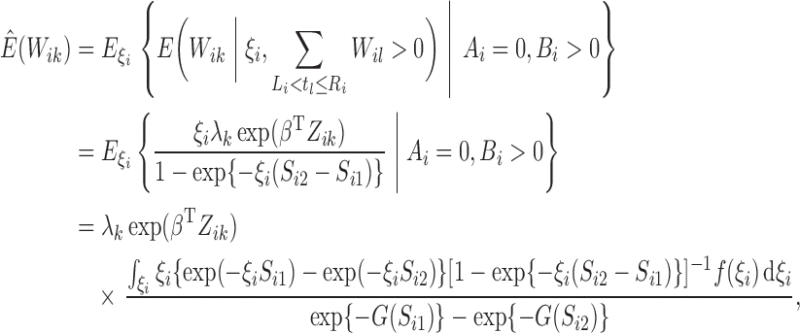 |
which can be calculated using Gaussian–Laguerre quadrature. In addition,
 |
where  for any function
  .
.
We iterate between the E- and M-steps until the sum of the absolute differences of the
estimates at two successive iterations is less than, say,  . This EM
algorithm has several desirable features. First, the conditional expectations in the
E-step involve at most one-dimensional integration, so they can be evaluated accurately by
Gaussian quadrature. Second, in the M-step, the high-dimensional parameters
. This EM
algorithm has several desirable features. First, the conditional expectations in the
E-step involve at most one-dimensional integration, so they can be evaluated accurately by
Gaussian quadrature. Second, in the M-step, the high-dimensional parameters

 are calculated
explicitly, while the low-dimensional parameter vector
are calculated
explicitly, while the low-dimensional parameter vector  is updated
by the Newton–Raphson method. In this way, the algorithm avoids the inversion of any
high-dimensional matrices. Finally, the observed-data likelihood is guaranteed to increase
after each iteration. To avoid local maxima, we suggest using a range of initial values
for
is updated
by the Newton–Raphson method. In this way, the algorithm avoids the inversion of any
high-dimensional matrices. Finally, the observed-data likelihood is guaranteed to increase
after each iteration. To avoid local maxima, we suggest using a range of initial values
for  while setting
  to
to  . We denote the
final results by
. We denote the
final results by  .
.
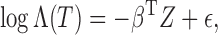
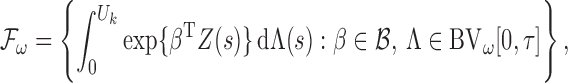
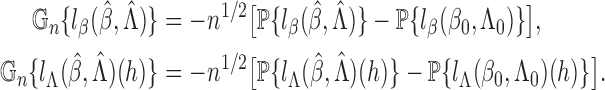
2.3. Variance estimation
We use profile likelihood (Murphy & van der
Vaart, 2000) to estimate the covariance matrix of  .
Specifically, we define the profile loglikelihood
.
Specifically, we define the profile loglikelihood
 |
where  is the set
of step functions with nonnegative jumps at
is the set
of step functions with nonnegative jumps at  . Then the covariance matrix of
 is estimated by the negative inverse of the matrix
whose
is estimated by the negative inverse of the matrix
whose  th element is
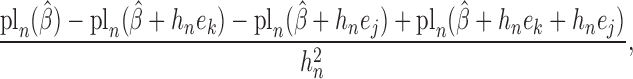 |
where  is the
 th canonical vector in
  and
and
 is a constant of order
  . To
calculate
. To
calculate  for each
  , we reuse the proposed EM
algorithm with
, we reuse the proposed EM
algorithm with  held fixed. Thus, the only step in the EM algorithm is
to explicitly evaluate
held fixed. Thus, the only step in the EM algorithm is
to explicitly evaluate  and
and  so as
to update
so as
to update  using (6). The iteration converges quickly with
  as
the initial value.
as
the initial value.
3. Asymptotic theory
We establish the asymptotic properties of  under the
following regularity conditions.
under the
following regularity conditions.
Condition 1. —
The true value of
, denoted by
, lies in the interior of a known compact set
in
, and the true value of
, denoted by
, is continuously differentiable with positive derivatives in
, where
is the union of the supports of
.
Condition 2. —
The vector
is uniformly bounded with uniformly bounded total variation over
, and its left limit exists for any
. In addition, for any continuously differentiable function
, the expectations
are continuously differentiable in
, where
and
are increasing functions in the decomposition
.

Condition 3. —
If
for all
with probability 1, then
for
and
.
Condition 4. —
The number of monitoring times,
, is positive, and
. The conditional probability
is greater than some positive constant
. In addition,
for some positive constant
. Finally, the conditional densities of
given
and
, denoted by
, have continuous second-order partial derivatives with respect to
and
when
and are continuously differentiable with respect to
.
Condition 5. —
The transformation function
is twice continuously differentiable on
with
,
and
.
Remark 2. —
Condition 1 is standard in survival analysis. Condition 2 allows
to have discontinuous trajectories, but the expectation of any smooth functional of
must be differentiable. One example would be that
is a stochastic process with a finite number of piecewise-smooth trajectories, where the discontinuity points have a continuous joint distribution. This condition excludes taking Brownian motion as a process for
. Condition 3 holds if the matrix
is nonsingular for some
. Condition 4 pertains to the joint distribution of monitoring times. First, it requires that the monitoring occur anywhere in
and that the largest monitoring time be equal to
with positive probability. The latter assumption may be removed, at the expense of more complicated proofs. Condition 4 also requires that two adjacent monitoring times be separated by at least
; otherwise, the data may contain exact observations, which would entail a different theoretical treatment. The smoothness condition for the joint density of monitoring times is used to prove the Donsker property of some function classes and the smoothness of the least favourable direction. Finally, Condition 5 pertains to the transformation function and holds for both the logarithmic family
and the Box–Cox family
.
The following theorem establishes the strong consistency of  .
.
Theorem 1. —
Under Conditions 1–5,
almost surely as
, where
is the Euclidean norm.
It is implicitly assumed in Theorem 1 that  is restricted to
 , although in practice
  is allowed
to be very large. The proof of Theorem 1 is based on the Kullback–Leibler information and
makes use of the strong consistency of empirical processes. Careful arguments are needed to
establish a preliminary bound for
is allowed
to be very large. The proof of Theorem 1 is based on the Kullback–Leibler information and
makes use of the strong consistency of empirical processes. Careful arguments are needed to
establish a preliminary bound for  and to handle
time-dependent covariates. Our next theorem establishes the asymptotic normality and
semiparametric efficiency of
and to handle
time-dependent covariates. Our next theorem establishes the asymptotic normality and
semiparametric efficiency of  .
.
Theorem 2. —
Under Conditions 1–5,
converges in distribution as
to a zero-mean normal random vector whose covariance matrix attains the semiparametric efficiency bound.
The proof of Theorem 2 relies on the derivation of the least favourable submodel for
 and utilizes modern empirical process theory. A key step
is to show that
and utilizes modern empirical process theory. A key step
is to show that  converges to
  at the
 rate. Although the general procedure is similar to
that of Huang & Wellner (1997), a major
innovation is the derivation of the least favourable submodel for general interval censoring
and time-dependent covariates by carefully handling the trajectories of
rate. Although the general procedure is similar to
that of Huang & Wellner (1997), a major
innovation is the derivation of the least favourable submodel for general interval censoring
and time-dependent covariates by carefully handling the trajectories of
 and the joint distribution of
  . The
existence of the least favourable submodel is also used at the end of the Appendix to show
consistency of the profile-likelihood covariance estimator given in §2.3.
. The
existence of the least favourable submodel is also used at the end of the Appendix to show
consistency of the profile-likelihood covariance estimator given in §2.3.
4. Simulation studies
We conducted simulation studies to assess the operating characteristics of the proposed
numerical and inferential procedures. In the first study, we considered two time-independent
covariates,  and
and  . In the second study, we allowed
 to vary over time by imitating two-stage randomization:
 , where
  and
and
 are independent
  and
and  with
with
 . In both studies, we generated the failure times from the
transformation model
. In both studies, we generated the failure times from the
transformation model
 |
where

 . We set
 ,
,  and
and
 . To create interval censoring, we randomly generated
two monitoring times,
. To create interval censoring, we randomly generated
two monitoring times,  and
and  , so that the time axis
 was partitioned into three intervals,
 ,
,  and
and  . On
average, there were 25–35% left-censored observations and 50–60% right-censored ones. We set
. On
average, there were 25–35% left-censored observations and 50–60% right-censored ones. We set
 , 400 or 800 and used 10 000 replicates for each
sample size.
, 400 or 800 and used 10 000 replicates for each
sample size.
For each dataset, we applied the proposed EM algorithm by setting the initial value of
 to 0 and the initial value of
  to
to
 , and we set the convergence threshold to
 . We also tried other initial values for
 , but they all led to the same estimates. For the variance
estimation, we set
, but they all led to the same estimates. For the variance
estimation, we set  , but the results differed only in the third
decimal place if we used
, but the results differed only in the third
decimal place if we used  or
or  . There was
no nonconvergence in any of the EM iterations.
. There was
no nonconvergence in any of the EM iterations.
Tables 1 and 2 summarize the results of the two simulation studies under
 or 1. The parameter estimators have small bias, and the
bias decreases rapidly as
or 1. The parameter estimators have small bias, and the
bias decreases rapidly as  increases. The variance estimators accurately reflect
the true variabilities, and the confidence intervals have proper coverage probabilities. As
shown in Fig. 1, the estimated cumulative hazard
functions have negligible bias.
increases. The variance estimators accurately reflect
the true variabilities, and the confidence intervals have proper coverage probabilities. As
shown in Fig. 1, the estimated cumulative hazard
functions have negligible bias.
Table 1.
Summary statistics for the simulation study with time-independent covariates

|

|

|
||||||||||||||

|
Est | SE | SEE | CP | Est | SE | SEE | CP | Est | SE | SEE | CP | ||||
| 0 |

|
0 515 515 |
0 209 209 |
0 216 216 |
96 | 0 506 506 |
0 148 148 |
0 149 149 |
95 | 0 503 503 |
0 103 103 |
0 104 104 |
95 | |||

|
 515 515 |
0 366 366 |
0 354 354 |
94 |
 505 505 |
0 254 254 |
0 248 248 |
95 |
 504 504 |
0 176 176 |
0 174 174 |
95 | ||||

|

|
0 514 514 |
0 255 255 |
0 259 259 |
96 | 0 507 507 |
0 180 180 |
0 176 176 |
94 | 0 503 503 |
0 125 125 |
0 125 125 |
95 | |||

|
 516 516 |
0 451 451 |
0 434 434 |
94 |
 505 505 |
0 311 311 |
0 303 303 |
94 |
 503 503 |
0 215 215 |
0 212 212 |
94 | ||||
| 1 |

|
0 516 516 |
0 294 294 |
0 297 297 |
95 | 0 506 506 |
0 209 209 |
0 207 207 |
95 | 0 504 504 |
0 145 145 |
0 144 144 |
95 | |||

|
 517 517 |
0 522 522 |
0 503 503 |
94 |
 505 505 |
0 358 358 |
0 350 350 |
95 |
 502 502 |
0 249 249 |
0 244 244 |
94 | ||||
Est, empirical average of the parameter estimator; SE, standard error of the parameter estimator; SEE, empirical average of the standard error estimator; CP, empirical coverage percentage of the 95% confidence interval.
Table 2.
Summary statistics for the simulation study with time-dependent covariates

|

|

|
||||||||||||||

|
Est | SE | SEE | CP | Est | SE | SEE | CP | Est | SE | SEE | CP | ||||
| 0 |

|
0 529 529 |
0 241 241 |
0 239 239 |
95 | 0 518 518 |
0 166 166 |
0 164 164 |
95 | 0 509 509 |
0 114 114 |
0 114 114 |
95 | |||

|
 515 515 |
0 363 363 |
0 353 353 |
95 |
 511 511 |
0 253 253 |
0 247 247 |
94 |
 503 503 |
0 175 175 |
0 173 173 |
95 | ||||

|

|
0 533 533 |
0 292 292 |
0 280 280 |
94 | 0 522 522 |
0 198 198 |
0 193 193 |
94 | 0 511 511 |
0 138 138 |
0 134 134 |
94 | |||

|
 514 514 |
0 441 441 |
0 433 433 |
95 |
 512 512 |
0 307 307 |
0 302 302 |
95 |
 503 503 |
0 214 214 |
0 211 211 |
95 | ||||
| 1 |

|
0 537 537 |
0 336 336 |
0 317 317 |
94 | 0 525 525 |
0 228 228 |
0 219 219 |
94 | 0 514 514 |
0 157 157 |
0 152 152 |
94 | |||

|
 518 518 |
0 512 512 |
0 502 502 |
95 |
 513 513 |
0 358 358 |
0 349 349 |
95 |
 505 505 |
0 250 250 |
0 243 243 |
94 | ||||
Fig. 1.

Estimation of  with
with  , for (a)
 and (b)
  . The solid and
dashed curves represent the true values and mean estimates, respectively.
. The solid and
dashed curves represent the true values and mean estimates, respectively.
We conducted an additional simulation study with five covariates. We set
 to zero-mean normal with unit variances and pairwise
correlations of 0
to zero-mean normal with unit variances and pairwise
correlations of 0 5 and took
  ; the other simulation settings were left unchanged. The
results are summarized in the Supplementary Material. The proposed methods performed well in
this simulation too. Again, there were no cases of nonconvergence.
; the other simulation settings were left unchanged. The
results are summarized in the Supplementary Material. The proposed methods performed well in
this simulation too. Again, there were no cases of nonconvergence.
To evaluate the performance of the EM algorithm in even larger datasets, we set
 and
and  to ten standard normal random variables
with pairwise correlations of 0
to ten standard normal random variables
with pairwise correlations of 0 25 and regression coefficients of
0
25 and regression coefficients of
0 5. The algorithm converged to values close to
0
5. The algorithm converged to values close to
0 5 in all 10 000 replicates.
5. Application
The Bangkok Metropolitan Administration conducted a cohort study of 1209 injecting drug users who were initially sero-negative for the HIV-1 virus. Subjects from 15 drug treatment clinics were followed from 1995 to 1998. At study enrolment and approximately every four months thereafter, subjects were assessed for HIV-1 sero-positivity through blood tests. As of December 1998 there were 133 HIV-1 sero-conversions and roughly 2300 person-years of follow-up.
We aim to identify the factors that influence HIV-1 infection. We fit model (1) with the class of logarithmic
transformations 
 . The
covariates include age at recruitment, gender, history of needle sharing, and drug injection
in jail before recruitment; age is measured in years, gender takes value 1 for male and 0
for female, and history of needle sharing and drug injection are binary indicators of yes or
no. In addition, we include a time-dependent covariate indicating imprisonment since the
last clinic visit.
. The
covariates include age at recruitment, gender, history of needle sharing, and drug injection
in jail before recruitment; age is measured in years, gender takes value 1 for male and 0
for female, and history of needle sharing and drug injection are binary indicators of yes or
no. In addition, we include a time-dependent covariate indicating imprisonment since the
last clinic visit.
To select a transformation function, we vary  from 0 to 1
 5 in steps of
0
5 in steps of
0 05. For each
  , we estimate
  and
and
 by the EM algorithm and evaluate the loglikelihood at the
parameter estimates. Figure 2(a) shows that the
loglikelihood changes only very slowly as
by the EM algorithm and evaluate the loglikelihood at the
parameter estimates. Figure 2(a) shows that the
loglikelihood changes only very slowly as  varies and is maximized at
 . We choose
  , which corresponds to the
proportional odds model. Table 3 shows the
results under this model. For comparison, we also include the results for
, which corresponds to the
proportional odds model. Table 3 shows the
results under this model. For comparison, we also include the results for
 , which corresponds to the proportional hazards model.
Fig. 2.

Analysis of the Bangkok Metropolitan Administration HIV-1 study: (a) the loglikelihood
at the nonparametric maximum likelihood estimates plotted as a function of
 in the logarithmic transformations; (b) estimation of
infection-free probabilities, where the upper lines correspond to a low-risk subject
under the proportional hazards (solid) and proportional odds (dashed) models, and the
lower lines correspond to a high-risk subject under the proportional hazards (solid) and
proportional odds (dashed) models.
in the logarithmic transformations; (b) estimation of
infection-free probabilities, where the upper lines correspond to a low-risk subject
under the proportional hazards (solid) and proportional odds (dashed) models, and the
lower lines correspond to a high-risk subject under the proportional hazards (solid) and
proportional odds (dashed) models.
Table 3.
Regression analysis of the Bangkok Metropolitan Administration HIV-1 infection data
| Proportional hazards | Proportional odds | |||||||
| Covariates | Estimate | Standard error |
 -value -value |
Estimate | Standard error |
 -value -value |
||
| Age |
 028 028 |
0 012 012 |
0 021 021 |
 031 031 |
0 013 013 |
0 016 016 |
||
| Gender | 0 424 424 |
0 270 270 |
0 117 117 |
0 539 539 |
0 310 310 |
0 082 082 |
||
| Needle sharing | 0 237 237 |
0 183 183 |
0 196 196 |
0 251 251 |
0 196 196 |
0 200 200 |
||
| Drug injection | 0 313 313 |
0 184 184 |
0 089 089 |
0 360 360 |
0 198 198 |
0 069 069 |
||
| Imprisonment over time | 0 502 502 |
0 211 211 |
0 017 017 |
0 494 494 |
0 219 219 |
0 024 024 |
||
Under either model, ageing reduces the risk of HIV-1 infection, whereas being male increases it. In addition, drug injection increases the risk. Finally, subjects who have recently been imprisoned have an elevated risk of HIV-1 infection.
Figure 2(b) shows the prediction of HIV-1 infection for a low-risk subject versus a high-risk subject. The low-risk subject is a 50-year-old female with no history of needle sharing, no drug injection in jail before recruitment, and no imprisonment during follow-up; the high-risk subject is a 20-year-old male with a history of needle sharing, drug injection in jail before recruitment, and imprisonment over time. The estimated probabilities of infection for the low-risk subject are similar under the proportional odds and proportional hazards models. For the high-risk subject, however, the proportional odds model yields slightly higher risks of infection than the proportional hazards model during the first part of the follow-up period, with the opposite being true during the later part of the follow-up period.
6. Remarks
The presence of time-dependent covariates poses major computational and theoretical
challenges. With time-dependent covariates, the parameters  and
and

 in the likelihood
function are entangled. As a result, the diagonal approximation to the Hessian matrix in the
iterative convex minorant algorithm (Huang &
Wellner, 1997) is inaccurate, and the algorithm becomes unstable. By contrast, each
iteration of our EM algorithm only solves a low-dimensional equation for
in the likelihood
function are entangled. As a result, the diagonal approximation to the Hessian matrix in the
iterative convex minorant algorithm (Huang &
Wellner, 1997) is inaccurate, and the algorithm becomes unstable. By contrast, each
iteration of our EM algorithm only solves a low-dimensional equation for
 while calculating the jump sizes of
 explicitly as weighted sums of Poisson rates. Thus, our
algorithm is fast and stable. In extensive numerical studies we have never encountered
nonconvergence. Our software is available at http://dlin.web.unc.edu/software.
explicitly as weighted sums of Poisson rates. Thus, our
algorithm is fast and stable. In extensive numerical studies we have never encountered
nonconvergence. Our software is available at http://dlin.web.unc.edu/software.
Our theoretical development requires that the population average of the covariate process
be smooth but allows individual covariate trajectories to be discontinuous. We treat
 as a bundled process of
 and
and  when proving the identifiability
of
when proving the identifiability
of  in Theorem 1, the convergence rate of
 in Lemma A1, and the invertibility of the information
operator in Theorem 2. The Donsker property for this class of processes indexed by
in Lemma A1, and the invertibility of the information
operator in Theorem 2. The Donsker property for this class of processes indexed by
 is used repeatedly in the proofs. Besides time-dependent
covariates, one major theoretical challenge is dealing with general interval censoring,
which allows each subject to have a different number of monitoring times. In particular, the
derivation of the least favourable direction for
is used repeatedly in the proofs. Besides time-dependent
covariates, one major theoretical challenge is dealing with general interval censoring,
which allows each subject to have a different number of monitoring times. In particular, the
derivation of the least favourable direction for  requires
careful consideration of the joint distribution for an arbitrary sequence of monitoring
times, and the Lax–Milgram theorem is used to prove the existence of a least favourable
direction. That theorem greatly simplifies the proof, in contrast to the approach of Huang & Wellner (1997), even for case-2
data.
requires
careful consideration of the joint distribution for an arbitrary sequence of monitoring
times, and the Lax–Milgram theorem is used to prove the existence of a least favourable
direction. That theorem greatly simplifies the proof, in contrast to the approach of Huang & Wellner (1997), even for case-2
data.
To apply the transformation model to real data, one must choose a transformation function. In the analysis of the Bangkok Metropolitan Administration HIV-1 data, we used the aic to select the transformation function, although the likelihood surface is fairly flat. It would be worthwhile to develop formal diagnostic procedures to check the appropriateness of the transformation function and other model assumptions. One possible strategy is to examine the behaviour of the posterior mean of the martingale residuals (Chen et al., 2012) given the observed intervals.
In many applications, the event of interest may occur repeatedly over time. Recurrent events under interval censoring are called panel count data, which have been studied by Sun & Wei (2000), Zhang (2002) and Wellner & Zhang (2007), among others. There are also studies in which each subject can experience different types of events or where subjects are sampled in clusters such that the failure times with the same cluster are correlated. We are currently developing regression methods to handle such multivariate failure time data.
We are also extending our work to competing risks data. Indeed, the Bangkok Metropolitan Administration HIV-1 study contains information on HIV-1 infection by viral subtypes B and E, which are two competing risks. We propose to formulate the effects of potentially time-dependent covariates on the cumulative incidence functions of competing risks in the form of model (1). We will modify the EM algorithm to deal with multiple subdistribution functions and establish the asymptotic theory under suitable conditions.
Supplementary material
Supplementary Material
Acknowledgments
This research was supported by the U.S. National Institutes of Health. The authors thank the editor, an associate editor and a referee for helpful comments.
Appendix A. Appendix
Technical details
We use  to denote the empirical measure from
 independent observations and
 to denote the true probability measure. The
corresponding empirical process is
to denote the true probability measure. The
corresponding empirical process is  . Let
. Let  be the
observed-data loglikelihood for a single subject, that is,
be the
observed-data loglikelihood for a single subject, that is,
 |
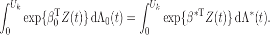
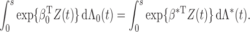
Proof of Theorem 1. —
We first show that
with probability 1. By Condition 4, the measure generated by the function
is dominated by the sum of the Lebesgue measure in
and the counting measure at
, and its Radon–Nikodym derivative, denoted by
, is bounded away from zero. We define
Clearly,
is a step function with jumps only at
. Since
uniformly in
with probability 1 as
, we conclude that
converges uniformly to
with probability 1 for
.
By the definition of
, we have
. Because of its bounded total variation,
belongs to a Donsker class indexed by
. Hence, the class of functions
where
denotes functions which have total variation in
bounded by a given constant
, is a convex hull of functions
, so it is a Donsker class. Furthermore,
is bounded away from zero. Therefore,
belongs to some Donsker class due to the preservation property of the Donsker class under Lipschitz-continuous transformations. We conclude that
almost surely. In addition, by the construction of
,
converges almost surely to
, which is finite. Therefore, with probability 1,
(A1) Let
be such that
for
. Then the left-hand side of (A1) is less than or equal to
Hence
. Since as
,
, which is positive, Condition 5 implies that
with probability 1.
We can now restrict
to a class of functions with uniformly bounded total variation, equipped with the weak topology on
. By Helly's selection lemma, for any subsequence of
we can choose a further subsequence such that
converges weakly to some
on
,
converges to
, and
converges to
. Clearly,
implies that
, where
, so that
By the above arguments for proving the Donsker property of
, together with the fact that the total variation of
is bounded by a constant, we can show that
belongs to a Donsker class with a bounded envelope function, so that
. It follows that
Furthermore,
where
is the measure corresponding to
. According to Conditions 2 and 4,
is dominated by the Lebesgue measure with bounded derivative in
and has a point mass at
. Hence
almost surely. We therefore conclude that
By the properties of the Kullback–Leibler information,
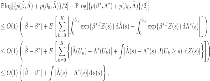
with probability 1. In particular, for any
, we choose
to obtain
Thus, for any
,
(A2) Differentiating both sides with respect to
, we have
By Condition 3,
and
for
. We let
by redefining
to centre at a deterministic function in the support of
, and we set
in (A2) to obtain
. Hence,
for
. It follows that
and
converges weakly to
almost surely. The latter convergence can be strengthened to uniform convergence since
is continuous. Thus, we have proved Theorem 1. □


Since we have established consistency, we may restrict the space of
 to
to
 |
for some  . Thus, when
 is large enough,
  belongs to
  with probability 1. Before proving Theorem 2, we need
to establish the convergence rate for
with probability 1. Before proving Theorem 2, we need
to establish the convergence rate for  . Specifically, the
following lemma holds.
. Specifically, the
following lemma holds.
Lemma A1. —
Under Conditions 1–5,
Proof. —
The proof relies on the convergence-rate result in Theorem 3.4.1 of van der Vaart & Wellner (1996). To use that theorem, we define
and let
be a class of functions indexed by
and
.
We first calculate the
-bracketing number of
. Because
consists of increasing and uniformly bounded functions on
, Lemma 2.2 of van de Geer (2000) implies that for any
, the bracketing number satisfies
where
denotes the
-norm with respect to the Lebesgue measure on
, and
means that
for a positive constant
. For
, we can find
number of brackets
with
and
to cover
. In addition, there are
number of brackets covering
, such that any two
within the same bracket differ by at most
. Hence, there are a total of
brackets covering
. For any pair of
and
, there exist some constants
and
such that
Because the measures
and
have bounded derivatives with respect to the Lebesgue measure in
and the former has a finite point mass at
,
Thus, the bracketing number for
satisfies
and so it has a finite entropy integral. Define
It is easy to show that
. In addition, by Lemma 1.3 of van de Geer (2000),
where
is the Hellinger distance, defined as
with respect to the dominating measure
.
The above results, together with the fact that
maximizes
and the consistency result in Theorem 1, imply that all the conditions in Theorem 3.4.1 of van der Vaart & Wellner (1996) hold. Thus, we conclude that
, where
satisfies
. In particular, we can choose
in the order of
such that
. By the mean value theorem,
On the left-hand side of the above equation, we consider the event
to find that
Next, we consider
to obtain the same equation as the one above but with
replaced by
. By repeating this process, we conclude that, conditional on
and for any
,
It then follows from the mean value theorem that
and so the lemma is proved. □


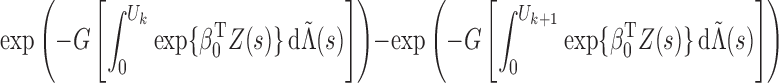
Now we are ready to prove Theorem 2.
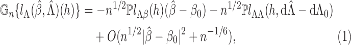
Proof of Theorem 2. —
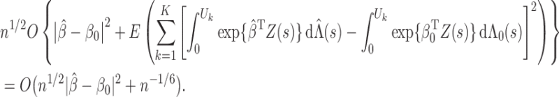
It is helpful to introduce the following notation:
,
and
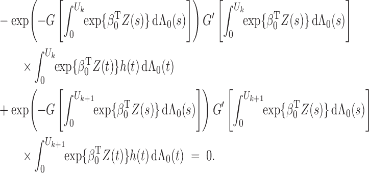
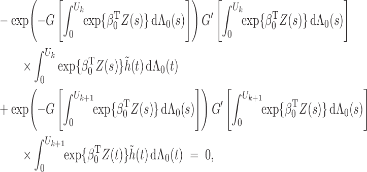
The score function for
is
To obtain the score operator for
, we consider any parametric submodel of
defined by
, where
. The score function along this submodel is
Clearly,
and
. Hence
We apply Taylor series expansions about
to the right-hand sides of the above two equations. By Lemma A1, the second-order terms are bounded by
Hence
(A3)
(A4) where
is the second derivative of
with respect to
,
is the derivative of
along the submodel
,
is the derivative of
with respect to
, and
is the derivative of
along the submodel
. All the derivatives on the right-hand sides of (A3) and (A4) are evaluated at
.
We choose
to be the least favourable direction
, a
-vector with components in
that solves the normal equation
(A5) where
is the adjoint operator of
. Then
so that the difference between (A3) and (A4) yields
(A6) Consequently, Theorem 2 will be established if we can show that:
equation (A5) has a solution
;
belongs to a Donsker class and converges in the
-norm to
;
the matrix
is invertible.
The reason is that when (i)–(iii) hold, (A6) entails
and further yields
This implies that the influence function for
is exactly the efficient influence function, so that
converges to a zero-mean normal random vector whose covariance matrix attains the semiparametric efficiency bound (Bickel et al., 1993, p. 65).
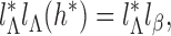
We first verify (i). For any
,
where
Likewise,
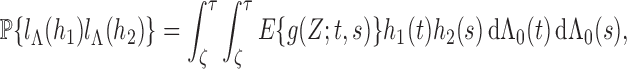
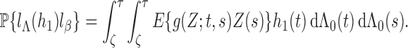
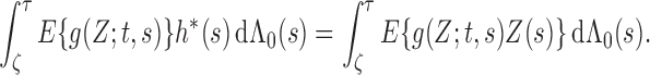
Therefore, by the definition of the dual operator
, solving the normal equation (A2) is equivalent to solving the integral equation
(A7) We define the left-hand side of (A7) as a linear operator
which maps
to itself. In addition, we equip
with an inner product
so that it becomes a Hilbert space. On the same space, we define
. It is easy to show that
is a seminorm for
. Furthermore, if
, then
. Thus, with probability 1,
is zero, i.e., for any
,
Setting
we obtain
Thus,
for
, implying that
is a norm in
. Clearly,
for some constant
. According to the bounded inverse theorem in Banach spaces, we have
for another constant
; that is, we have
. By the Lax–Milgram theorem (Zeidler, 1995), the solution to (A7), namely
exists. So we have verified (i).
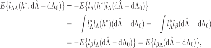
To verify (ii), we examine
by considering
and
. Along the lines of Huang & Wellner (1997), we differentiate the integral equation (A7) with respect to
to obtain
where
and
are continuously differentiable with respect to their arguments. Hence
is continuously differentiable in
. This fact implies that
belongs to some Donsker class. It then follows from the Donsker property of the class
that (ii) is true.
Finally, we verify (iii). If the matrix is singular, then there exists a nonzero vector
such that
It follows that, with probability 1, the score function along the submodel
is zero; that is, for any
,
where
. We consider
for
to obtain
Therefore, with probability 1,
for any
. This implies that
, so
by Condition 3. Thus, we have verified (iii). □


Remark A1. —
For a given
, we define
as the step function that maximizes
. The arguments in the proof of Theorem 1 can be used to show that
is bounded asymptotically when
is in a small neighbourhood of
, so
converges to
as
converges to
. In addition, the arguments in the proof of Lemma A1 yield
in the
space. Finally, in light of the existence of
in the proof of Theorem 2, we can define
to obtain the least favourable submodel as
, where
is in a neighbourhood of
. Thus, we can easily verify conditions (8), (9) and (10) of Murphy & van der Vaart (2000) for the likelihood function along this submodel. Along with the Donsker property of the functional classes for the first and second derivatives of
with respect to
and
, we conclude that Theorem 1 of Murphy & van der Vaart (2000) is applicable, and hence the covariance matrix estimator given in §2.3 with
is consistent for the limiting covariance matrix of
.
References
- Bickel P. J., Klaassen C. A. J., Ritov Y. & Wellner J. A. (1993). Efficient and Adaptive Estimation for Semiparametric Models. Baltimore: Johns Hopkins University Press. [Google Scholar]
- Chen K., Jin Z. & Ying Z. (2002). Semiparametric analysis of transformation models with censored data. Biometrika 89, 659–68. [Google Scholar]
- Chen L., Lin D. Y. & Zeng D. (2012). Checking semiparametric transformation models with censored data. Biostatistics 13, 18–31. [DOI] [PMC free article] [PubMed] [Google Scholar]
- Gu M. G., Sun L. & Zuo G. (2005). A baseline-free procedure for transformation models under interval censorship. Lifetime Data Anal. 11, 473–88. [DOI] [PubMed] [Google Scholar]
- Huang J. (1995). Maximum likelihood estimation for proportional odds regression model with current status data. In Analysis of Censored Data, vol. 27 of IMS Lecture Notes—Monograph Series, H. L. Koul and J. V. Deshpande, eds. Hayward: Institute of Mathematical Statistics, pp. 129–46.
- Huang J. (1996). Efficient estimation for the proportional hazards model with interval censoring. Ann. Statist. 24, 540–68. [Google Scholar]
- Huang J. & Rossini A. J. (1997). Sieve estimation for the proportional-odds failure-time regression model with interval censoring. J. Am. Statist. Assoc. 92, 960–7. [Google Scholar]
- Huang J. & Wellner J. A. (1997). Interval censored survival data: A review of recent progress. In Proc. 1st Seattle Symp. Biostatist.: Survival Anal., D. Y. Lin and T. R. Fleming, eds. New York: Springer, pp. 123–69.
- Murphy S. A. & van der Vaart A. W. (2000). On profile likelihood. J. Am. Statist. Assoc. 95, 449–65. [Google Scholar]
- Rabinowitz D., Betensky R. A. & Tsiatis A. A. (2000). Using conditional logistic regression to fit proportional odds models to interval censored data. Biometrics 56, 511–8. [DOI] [PubMed] [Google Scholar]
- Rossini A. J. & Tsiatis A. A. (1996). A semiparametric proportional odds regression model for the analysis of current status data. J. Am. Statist. Assoc. 91, 713–21. [Google Scholar]
- Schick A. & Yu Q. (2000). Consistency of the GMLE with mixed case interval-censored data. Scand. J. Statist. 27, 45–55. [Google Scholar]
- Shen X. (1998). Proportional odds regression and sieve maximum likelihood estimation. Biometrika 85, 165–77. [Google Scholar]
- Sun J. & Sun L. (2005). Semiparametric linear transformation models for current status data. Can. J. Statist. 33, 85–96. [Google Scholar]
- Sun J. & Wei L. J. (2000). Regression analysis of panel count data with covariate-dependent observation and censoring times. J. R. Statist. Soc. B 62, 293–302. [Google Scholar]
- van de Geer S. A. (2000). Empirical Process Theory and Applications. Cambridge: Cambridge University Press. [Google Scholar]
- van der Vaart A. W. & Wellner J. A. (1996) Weak Convergence and Empirical Processes. New York: Springer. [Google Scholar]
- Wang L., McMahan C. S., Hudgens M. G. & Qureshi Z. P. (2015). A flexible, computationally efficient method for fitting the proportional hazards model to interval-censored data. Biometrics72, 222–31. [DOI] [PMC free article] [PubMed]
- Wellner J. A. & Zhang Y. (2007). Two likelihood-based semiparametric estimation methods for panel count data with covariates. Ann. Statist. 35, 2106–42. [Google Scholar]
- Zeidler E. (1995). Applied Functional Analysis: Applications to Mathematical Physics. New York: Springer. [Google Scholar]
- Zeng D. & Lin D. Y. (2006). Efficient estimation of semiparametric transformation models for counting processes. Biometrika 93, 627–40. [Google Scholar]
- Zhang Y. (2002). A semiparametric pseudolikelihood estimation method for panel count data. Biometrika 89, 39–48. [Google Scholar]
- Zhang Z. & Zhao Y. (2013). Empirical likelihood for linear transformation models with interval-censored failure time data. J. Mult. Anal. 116, 398–409. [Google Scholar]
- Zhang Z., Sun L., Zhao X. & Sun J. (2005). Regression analysis of interval-censored failure time data with linear transformation models. Can. J. Statist. 33, 61–70. [Google Scholar]
Associated Data
This section collects any data citations, data availability statements, or supplementary materials included in this article.