Spot size variation FCS in simulations of the 2D Ising model

Abstract

Spot variation fluorescence correlation spectroscopy (svFCS) was developed to study the movement and organization of single molecules in plasma membranes. This experimental technique varies the size of an illumination area while measuring correlations in time using standard fluorescence correlation methods. Frequently, this data is interpreted using the assumption that correlation measurements reflect the dynamics of single molecule motions, and not motions of the average composition. Here, we explore how svFCS measurements report on the dynamics of components diffusing within simulations of a 2D Ising model with a conserved order parameter. Simulated correlation functions report on both the fast dynamics of single component mobility and the slower dynamics of the average composition. Over a range of simulation conditions, a conventional svFCS analysis suggests the presence of anomalous diffusion even though single molecule motions are nearly Brownian in these simulations. This misinterpretation is most significant when the surface density of the fluorescent label is elevated, therefore we suggest future measurements be made over a range of tracer densities. Some simulation conditions reproduce qualitative features of published svFCS experimental data. Overall, this work emphasizes the need to probe membranes using multiple complimentary experimental methodologies in order to draw conclusions regarding the nature of spatial and dynamical heterogeneity in these systems.

INTRODUCTION

Experimental measurements of spatio and temporal correlations have shed light on the organization and dynamics of fluorescently tagged bio-molecules in a broad range of biological systems [1–6] [7]. These methods take advantage of the fact that single fluorescent molecules emit a continuous stream of photons as they move in space and time, making it possible to measure the average correlations of photons arriving at a detector. These techniques are powerful because data can be collected from a broad range of samples with good signal to noise, since generating correlation functions inherently involves averaging data acquired in time. These methods have been widely applied to studies of molecules in membranes, where they have been used to measure diffusion coefficients [8–10], quantify the oligomerization states of membrane proteins, detail time-dependent interactions between membrane proteins [11, 12], and document the heterogeneity of protein and lipid mobility in a range of different contexts [13–15]

Spot size variation fluorescence correlation spectroscopy (svFCS) [15–17] is an application of correlation methods where the beam-waist of a confocal spot is varied to identify how measured correlation functions depend on the area of excitation. For simple Brownian diffusion within a uniform two dimensional membrane, correlation functions produce a single diffusion time which varies linearly with excitation area. In addition, the linear slope of diffusion time vs. excitation area extrapolates to intersect the origin, meaning that single molecules can instantaneously transit across an infinitesimally small area. In practice, the minimum excitation area that can be probed is limited by the diffraction limit of visible light (0.6μm²), or in recent studies by the minimum effective excitation area within a STED beam (~1000nm²) [18]. Plots of diffusion time vs. excitation area can deviate from the simple expectations from Brownian motion when svFCS is applied to single molecule motions in intact cells [15, 18–21]. Typically these curves retain their linear slope, but extrapolate to a non-zero intercept at zero excitation area. This type of experiment has been used to infer the presence of structure in membranes on length-scales below those accessible in these measurements. Past work has demonstrated that transient pinning or partitioning into static domains yields a positive intercept, while corralled motion within a mesh gives rise to negative intercepts [16]. One goal of this work is to investigate how plots of transit time vs. excitation area vary for single molecules diffusing in a third model of a heterogeneous membrane, one in which extended regions of different protein and lipid composition form because the membrane composition is tuned to be slightly above a miscibility critical point at physiological temperature. These super-critical composition fluctuations have been observed in model membranes made of purified components [22] and those isolated from the plasma membranes of living cells [23], and are well described by predictions of the two dimensional (2D) Ising model [24, 25].

The use of correlation methods to infer single molecule dynamics can prove challenging in the limit where multiple molecules are visualized on the time-scale of an experiment. In these cases, other time-scales can emerge due to the dynamics of the average composition, which can in principle vary dramatically from single molecule motions. For example, in a densely labeled sample, variations in signal intensity with a fixed diffraction limited area represent changes in the density of the molecule of interest, and not the motions of single molecules. In a Brownian and uniform membrane, a densely labeled sample would yield a time-time correlation function with low amplitude, since signal intensity would not vary significantly with time. A membrane with structure that itself is dynamic, such as one that contains diffusing phase separated domains, would produce correlation functions that report time-scales reflecting the lifetime and/or mobility of these structures. A typical experiment falls somewhere between these two extremes, under conditions where both the dynamics of single molecules and the dynamics of the average composition are reflected in measured correlation functions. A second goal of this work is to investigate how this combination of single molecule and average composition dynamics impacts interpretations of svFCS data through simulations of the two dimensional (2D) Ising model.

One feature of super-critical systems such as the 2D Ising model is that the average concentration can exhibit slow dynamics even though single molecule mobility is only subtly impacted [26–30]. Here, we systematically vary both the size and life-time of composition fluctuations by adjusting temperature with respect to the critical temperature in this model. We also systematically vary the density of tracer components in the membrane in order to probe the cross-over regime where simulated FCS curves report on both single molecule and average composition dynamics.

METHODS

Ising model simulations

A two dimensional (2D) Ising model with a conserved order parameter was simulated at the temperatures and compositions indicated using standard Monte Carlo algorithms as described previously [24]. Simulations were conducted on a 400 by 400 pixel square lattice with periodic boundary conditions, with a pixel length corresponding to 2 nm. This calibration is chosen so that measurements of correlation length (ξ) vs. reduced temperature (T/T_C -1) matches experimental findings in model and isolated membranes [23, 24]. Initially, updates were performed using non-local exchanges to decrease equilibration times. After equilibration, updates were restricted to only nearest neighbor exchanges (Kawasaki dynamics [31]) in order to replicate diffusive motions, with moves that swap like pixels at the same attempt frequency as unlike pixels. In all cases, a random subset of components of a single type was designated as tracers and their positions reported at 1000 equally spaced time-intervals. Simulations were run at 3 different frame-times, 10, 100, and 1000 sweeps per update, in order to increase the dynamic range of the time interval τ (from 10 to 10⁶ sweeps). We use the conversion factor of 1μs per sweep so that the macroscopic diffusion coefficient (D) is close to 4 μm²/s for temperatures far from the critical point.

Calculating autocorrelation functions

Curves indicating fluorescence intensity vs. time were constructed by performing a dot product of a 2D Gaussian point spread function (PSF) with a matrix indicating tracer positions. To improve statistics, multiple well-spaced PSFs were generated from a single simulation, and multiple independent simulations (2–100) were conducted for the same conditions. Each time-trace was used to generate a time-time correlation function using Fast Fourier Transforms (FFTs) that are padded with zeros to avoid artefactual correlations arising from the periodic boundary conditions inherent to the FFT.

$$g(\tau )=\mathit{iFFT}\left({\left|\mathit{FFT}\left(I(t)-\langle I(t)\rangle \right)\right|}^2\right)/N(\tau )$$ (Eqn 1)

Correlation functions are normalized to be zero for an uncorrelated signal, and account for the finite duration of acquisition through the normalization factor N:

$$N(\tau )={\langle I(t)\rangle }^2\times \mathit{iFFT}\left({\left|\mathit{FFT}(M(t))\right|}^2\right)$$ (Eqn 2)

Where M(t) is a step function that is 1 everywhere and again this FFT is padded with zeros. The time average intensity <I(t)> was calculated from the density of tracers since this is a conserved quantity. I(t) was not tabulated from the data-trace itself because there were cases where simulations were not long enough to become uncorrelated. Individual correlation functions are then averaged from simulations conducted at the same frame-time (sweeps per update) and combined with curves obtained with simulations conducted with different frame-times. Error bars indicate the standard error of the mean between simulations conducted with the same frame-time.

Determining diffusion parameters from g(τ)

Simulated g(τ) curves were fit to multiple functional forms commonly used to fit experimental FCS data of membrane components [7, 18, 32]. These include a model of 2D Brownian motion from a single population of diffusing tracers:

$$g(\tau )=\frac{1}{N}\frac{1}{1+\tau /{\tau }_D}$$ (Eqn 3)

Here, N and τ_D are fit parameters. For Brownian motion, n is simply the density of tracers and τ_D is the average transit time across the illumination area. g(τ) curves were also fit to a model of two independent diffusing Brownian populations:

$$g(\tau )=\frac{1}{N_1}\frac{1}{1+\tau /{\tau }_{D1}}+\frac{1}{N_2}\frac{1}{1+\tau /{\tau }_{D2}}$$ (Eqn 4)

This model has 4 fit parameters, the density of tracers in each population (N₁ and N₂) and the transit times for each of these populations through the illuminated spot (τ_D1 and τ_D2). Finally, g(τ) curves were fit to a model of confined diffusion for a single population:

$$g(\tau )=\frac{1}{N}\frac{1}{1+{(\tau /{\tau }_D)}^{\alpha }}$$ (Eqn 5)

This model has three fit parameters: N, τ_D, and α, where α is commonly referred to as a confinement exponent. α=1 reduces to Eqn 3 which is unconfined Brownian motion. α<1 indicates that motions are confined in this model. In all cases, fitting was performed using the lsqnonlin fitting routine in Matlab and error bounds reflect 68% confidence intervals on determined fit parameters.

RESULTS

Diffusion was simulated with a range of tracer densities, ranging from 10 to 1000 tracers per 400 by 400 pixel (800 by 800nm) box. Lists of tracer locations vs. time were then converted into curves of intensity vs. time for multiple Gaussian shaped spot-sizes with standard deviations ranging from 1 to 25 pixels (2 to 50nm), as described in Methods. Figure 1 shows two examples where tracers undergo Brownian motion on an unstructured background but with different tracer densities (Figure 1 A and E). For the smallest spot-sizes, single tracers can be seen diffusing through the spot generating intermittent spikes in intensity and whose frequency depends on the tracer density (Figure 1 B and F). For larger spot-sizes, multiple fluorophores reside within the illuminated area and each tracer spends more time within the illuminated area, resulting in a more smoothly varying trace of intensity vs. time.

Figure 1. Simulating spot size dependent correlation functions for Brownian motion.

(A,E) Representative snap-shots of simulations conducted at low (A; 0.03%) and high (E; 0.6%) tracer densities. Tracers are drawn larger than their actual size for demonstration purposes. Images also depict the size and shape of several Gaussian illumination spots (40, 20, 10, and 4nm) standard deviations going from top to bottom. (B, F) Representative time-traces calculated by superimposing the illumination spot on the tracer distribution as described in Methods. Traces correspond to the same illumination areas and order shown in A, E. (C,G) Time-time autocorrelation functions, g(τ), tabulated from time-traces like those shown in B,F. The points shown are an average over multiple spot locations and simulations, and error bounds are smaller than the point dimensions. Lines are fits to Eqn 3 which describes Brownian motion in two dimensions. Fits report the mean transit time, τ_D, and the number of tracers per spot, N. (D,G) Plots of fit parameters vs. illumination area. τ_D varies linearly with area and intersects the origin, as expected for Brownian motion. The slope of this line is related to the diffusion coefficient as D = 1/(4 × slope) = 3.4μm²/s. N is converted into a % of tracers, ρ, which is independent of spot area, where ρ=N/(spot area) ×(box area)/(total number of components) ×100%. Simulations were conducted in the Ising model with T = 5×T_C

This qualitative behavior is reflected in the tabulated autocorrelation function, g(τ), as a function of time-interval (τ) assembled using many time-traces and simulations (Figure 1 C and G). For small spot-sizes, g(τ) decays quickly to zero. The decay of g(τ) extends to longer τ for larger spot-sizes, reflecting the longer time needed for single tracers to diffuse through the larger spot. g(τ) curves tabulated from these simulations are well fit by the expected model of Brownian Motion in two dimensions (2D) as reported in Eqn 3. These fits report on the transit time of tracers through the illuminated spot, τ _D, and the average number of tracers within the illuminated spot, N (Figure 1 D and G). The fit parameter τ _D varies linearly with illumination area, and reports on the diffusion coefficient (D) of single component mobility. D is close to 4μm²/s (3.4 μm²/s for these examples), a value in line with lipid mobility in cell plasma membranes measured at very fast time-scales [33, 34] or transmembrane peptide mobility in isolated plasma membranes [35], and was set by choosing the calibration for simulation time vs. real time in these computations. The best fit value of the other fit parameter, N, can be converted into a tracer density, ρ. This quantity does not vary with illumination area but does report on the different tracer densities used in the two simulations shown. We note that Eqn 3 and the tabulated curves in Figure 1 indicate that the shape of g(τ) does not depend on tracer density, but its amplitude varies inversely with density (compare 1 C and G).

The conserved order parameter 2D Ising model is a lattice model made up of two distinct types of components. This model undergoes a demixing transition at low temperature, where these two components phase separate. At high temperature, both components uniformly mix with no long-range structure. For systems with an equal number of each type of component, large composition fluctuations are found as temperature (T) is lowered towards the phase transition temperature, called the critical temperature or T_C. The size of fluctuations is characterized with the correlation length, ξ, which varies as ξ=(T/T_C-1)⁻¹, as seen in the representative simulation snapshots of Figure 2A. Larger composition fluctuations found near T_C also have longer life-times, with characteristic times which vary as (T/T_C-1)^−z with z being close to 4 for the dynamics employed in this study [29]. In this model, changes in temperature result in changes in the size and life-time of structure but only minor changes in the dynamics of single component motions [26–29]. Single component dynamics depend only on the frequency in which a component accepts a move to a neighboring pixel. This is based on the energetic cost (or gain) of the proposed switch, and is accepted nearly all of the time at elevated temperature and most of the time at lower temperature. Often times these two components of the dynamics of critical systems are referred to as tracer diffusion or self-diffusion and gradient diffusion [28, 30]. Tracer diffusion describes single component motions that are only weakly affected by proximity to the critical point, while gradient diffusion describes the dynamics of the average composition which slows dramatically near T_C. This slowing of gradient diffusion near T_C is often referred to as critical slowing down [29, 30].

Figure 2. Correlation functions of tracers in the Ising model vary with temperature and tracer density.

(A) Representative snap-shots of simulations conducted at the temperatures indicated and at fixed tracer density (ρ=0.16%). White tracers are a subset of orange pixels and are drawn larger than the pixels themselves for demonstration purposes. (B) Aggregate g(τ) curves for the temperatures and tracer density in A at a fixed spot area (corresponding to σ=10nm). Intensity at large τ becomes more pronounced at lower temperatures when composition fluctuations are large and long-lived. (C) Representative snap-shots of simulations conducted at fixed temperature (1.05×T_C) and varying tracer density as indicated. Aggregate g(τ) curves for the temperature and tracer densities in C at a fixed spot area (corresponding to σ=10nm). Intensity at short τ depends strongly on tracer density, but all curves decay to the same long τ behavior within signal to noise. (E) Snapshot of T=1.05×T_C and ρ=0.16% blurred with different Gaussian filters with standard deviations (σ) between 4 and 40nm. This represents the image that would be acquired with this beam size if the structure was static and if all ordered and disordered components were labeled. The color bar at right indicates density (orange = all ordered components; blue = all disordered components). Black circles have a radius of σ. (F) Aggregate g(τ) curves for simulations shown in E. The long τ tail of curves are not largely effected by the PSF size until σ exceeds the correlation length (ξ=20nm under these conditions). In B, D, and E the inset contains the same data plotted on a log-log scale.

Both the fast dynamics of single component motions and the slow dynamics of the average composition are apparent in tabulated correlation functions in the 2D Ising model near T_C. This can be seen in Figure 2B, where correlations due to single molecule motions appear at short τ. This component has roughly the same amplitude and range for all three curves shown because they were generated from simulations with the same tracer density and spot size. These curves differ in the amplitude of correlations at long τ. These long τ correlations arise from the slowly changing average composition in these simulations, which emerges as temperature approaches T_C.

Unlike tracer diffusion, whose correlations vary inversely with tracer density, contributions to the correlation function arising from gradient diffusion do not depend on density beyond affecting signal to noise because tracers randomly sample an underlying structure. This can be seen in Figure 2C and D where g(τ) is shown for 4 simulations run at the same temperature and spot size but with different tracer densities. These curves have dramatically different amplitudes at short τ, but converge to the same curve at longer τ. As a result, g(τ) curves for simulations with low tracer density are dominated by fast tracer diffusion. As tracer density is increased, g(τ) becomes increasingly dominated by the slowly varying correlations of the average composition.

Figure 2 also shows how g(τ) varies with illumination area for a simulation conducted close to T_C and with a high tracer density. Figure 2E shows how the structure present in the average composition becomes washed out as the spot size becomes larger than the average size of structure, which is ξ=20nm in this simulation. The correlation functions of Figure 2F demonstrate how g(τ) depends on illumination area under these conditions. As was the case for diffusion on in a much more uniform simulation, the amplitude of correlations at short τ due to tracer diffusion decrease as illumination area increases. This occurs because on average, more tracer molecules are present within each illumination spot and the amplitude of the correlation function goes as 1/N. The amplitude of correlations at long τ due to gradient diffusion has a more complicated dependence on illumination area. Fig 2F indicates that g(τ) is weakly dependent on illumination at long τ, for conditions where the illumination spot is smaller than the average size of structure in the simulation (ξ=20nm). When the illumination spot is larger than the average size of structure, the long τ tail of g(τ) is also attenuated. Overall, this suggests that g(τ) will become increasingly dominated by contributions from the average composition fluctuations until the spot size becomes much larger than this structure. For larger illumination areas, both contributions to g(τ) decrease in amplitude as area is increased.

Experimental studies utilizing svFCS typically fit acquired g(τ) curves to extract information on the average transit-time through the illumination area, then fit parameters are plotted as a function of illumination area. Individual g(τ) curves are often fit to models of either one or multiple Brownian populations (Eqns 3 and 4), or by fitting to a confined diffusion model that incorporates a confinement exponent α (Eqn 5). Figure 3A shows g(τ) for an Ising model simulated at T=1.1×T_C along with fits to all three models. The model of a single Brownian population (Eqn 3) fits these g(τ) poorly at short τ in order to accommodate the slow decay of these curves at larger τ. In contrast, both slow and fast decays of g(τ) are well fit when two diffusing populations are assumed (Eqn 4). The confined diffusion model (Eqn 5) is able to accommodate the slow decay of g(τ) curves for all but very short τ. In contrast, g(τ) curves from simulations are conducted at high temperature (T=5×T_C) are well fit by the model describing a single Brownian population for all illumination areas (Eqn 3; Figure 3B). We note that experimental g(τ) curves are often the least specified at short τ, in part due to statistics and in part due to non-diffusive contributions to the fluorescence correlation arising from the decay of the triplet excited state (e.g. [36]).

Figure 3. Fit parameters from simulated g(τ).

(A) Aggregate g(τ) curves from simulations conducted with T = 1.1×T_C and ρ=0.16% and the indicated illumination half-widths (σ). Lines are fits to a single Brownian population (Eqn 3; solid color), two Brownian populations (Eqn 4; solid black) and a single anomalous population (Eqn 5; dash color). (B) g(τ) curves for T = 5×T_C and ρ=0.16% at the same illumination half-widths. Solid line is a fit to a single Brownian population (Eqn 3). (C) Summary of fit parameters obtained for ρ=0.16% over the range of temperatures indicated. Fit parameters are described in Eqns 3–5 in Methods. At high temperatures, the four parameter fit of Eqn 4 is not well specified, therefore τ_D is replotted for τ_D1 and τ_D2 is not plotted for these conditions (T = 1.5×T_C, 5×T_C). (D) Summary of fit parameters obtained for T = 1.1×T_C over the range of tracer densities indicated. At the lowest tracer density shown τ_D is replotted for τ_D1 and τ_D2 is not plotted for (ρ=0.03%) because the fit to Eqn 4 was not well specified. The solid line in plots of τ_D vs area in C,D is a linear fit to τ_D points corresponding to areas between 5.6×10³ and 1.6 ×10⁴ nm². This line is extrapolated to area=0 to illustrate the positive y intercept.

Figure 3C and D show fit parameters as a function of illumination area for simulations conducted at fixed tracer density and varying temperature (Fig 3C) and fixed temperature and varying tracer density (Fig 3D). At fixed tracer density, correlation times increase with both illumination area and with decreasing temperature when curves are fit to a single Brownian diffuser model (τ_D). Close to T_C, transit times determined in this way are longer than those expected from tracer diffusion, due to the slowly varying average composition. In addition, plots of τ_D vs. illumination area are not linear. Instead, a line fit to larger area points extrapolates to a positive intercept at zero immunization area. In the svFCS literature, a similar curve would be interpreted as indicating that the tracer partitions into domains [15–17]. In this case, this effect occurs because the slowly varying average composition fluctuations impact the best fit transit times more greatly at large illumination areas compared to small illumination areas, making the curves nonlinear.

When curves are fit to two Brownian populations, each with their own transit time (τ_D1 and τ_D2), the tracer diffusion is reflected in the faster transit time (τ_D1), which varies linearly with illumination area as expected for Brownian motion. For the examples shown in Figure 3C, transit times for the second component (τ_D2) are orders of magnitude longer and do not necessarily vary linearly with illumination area. Best fit values for the confinement exponent α obtained by fitting to Eqn 5 also vary with temperature and to a lesser extent with illumination area. Confinement is greatest close to T_C and trends to 1 at high temperatures, in agreement with diffusion becoming Brownian under these conditions.

Plots of fit parameters vs. illumination area also depend on the tracer density, with larger densities leading to the appearance of greater anomalies at fixed temperature. This can be seen in the plots of the average transit time τ_D and of the confinement exponent α. This occurs because the correlation function becomes increasingly dominated by the slowly varying average composition as density is increased (Fig 2D). In contrast, when curves are fit such that tracer diffusion is isolated from the slowly varying average composition fluctuations, the τ_D1 again appears Brownian for all densities and τ_D1 and τ_D1 each collapse onto the same curve. The intensity of each of these components (captured in the parameters N₁ and N₂) vary as tracer density is varied.

We have generated curves like those shown in Figure 3C and 3D for simulations conducted over a range of temperatures and tracer densities to obtain the results summarized in Fig 4. Figure 4A and 4B are extracted from measurements of τ_D vs. illumination area by fitting large area points to a linear slope, as shown in several representative conditions in Figure 3C and 3D. Figure 4A reports the y intercept of this line, which is often interpreted as a measure of the level of confinement into domains [17]. The intercept is largest close to T_C and at larger tracer densities (Figure 4A), although the anomaly is still apparent at low tracer density close to T_C. The slope of the linear fit to τ_D vs area is often interpreted as reporting on the effective diffusion coefficient of single molecules according to the relation D_eff = 1/(4×slope) [17]. This quantity, plotted in Figure 4B, varies weakly with temperature and is largely independent of tracer density. This is also seen by directly observing the shapes of τ_D vs illumination area plots at varying density in Figure 3D.

Figure 4. Summary of svFCS fit parameters in the 2D Ising model.

(A) Extrapolated Y intercepts obtained by fitting plots of τ_D vs area, for areas between 5.6×10³ and 1.6 ×10⁴ nm² where τ_D is obtained by fitting to Eqn 3. (B) Effective diffusion coefficients (D_eff) defined as the inverse slope divided by 4 of the line described for part A. (C,D) Diffusion coefficients associated with the best fit values of τ_D1 (C) and τ_D2 (D) for σ=10nm (area = 630nm²) as determined from Eqn 4. (E) The inverse of the best fit value for the confinement exponent α as determined from Eqn 5.The value presented is an average over all areas. The legends in B,C apply to points in panels A–E and conditions are plotted only for instances where correlation functions and fits are well specified. (F) The characteristic size of composition fluctuations as a function of reduced temperature. For all temperatures probed, this correlation length is much smaller than the dimensions of the simulation box (800×800nm).

Figures 4 C and D report the results of fitting g(τ) to two populations of diffusers with two distinct transit times. These quantities are converted to diffusion coefficients D₁ and D₂ according to A = 4D₁τ_D1 and A = 4D₁τ_D1 where A was the specific illumination area of A=630nm². The fast component represented by D₁, varies weakly with temperature and has an absolute value that is similar to those reported in Figure 4B. This quantity describes single molecule motions in these simulations. In contrast, the slow component represented by D₂ varies dramatically with temperature, and becomes orders of magnitude slower than D₁ close to T_C. Note that the y axis is plotted on a linear scale in Figure 4C and a logarithmic scale in Figure 4D. This D₂ diffusion coefficient reflects on the slow dynamics of the average composition near T_C. Figure 4E shows how the confinement exponent α varies with temperature and tracer density averaged over all illumination areas probed. As expected, this confinement is most prominent at low temperatures and large tracer densities. In experiments, the parameter α tends to vary between. 5 and 1 (1<α⁻¹<2) [18, 32], which is observed routinely in simulations conducted using a wide range of conditions. We note that in these simulations, single components are not confined (e.g. plots of τ_D1 vary linearly with area and pass through the origin). Instead, they appear confined because the slow dynamics of the average composition is interpreted as a component of single molecule motion.

Within the ensemble of simulations conducted, there is a subset that shares qualitative features with experimental results presented in the literature [18]. One example is shown in Figure 5, which shows the emergence of a fast and slow time-scale in g(τ) curves constructed from time-traces at smaller illumination areas. This occurs when the diameter of the illumination area becomes much larger than the correlation length, such that the simulations appear unstructured at this length-scale. For the case of this simulation conducted at 1.2×T_C, the correlation length ξ is close to 5nm, and the slower component of g(τ) emerges for illumination areas roughly an order of magnitude larger than this in diameter (σ=25nm). At and below this same illumination area, g(τ) curves also exhibit confinement (1/α >1) when fit to Eqn 5. A similar trend has been observed experimentally for some lipid species probed in living cells [18, 32], although there are quantitative differences in the transit times and illumination areas where this transition occurs.

Figure 5. 2D Ising model simulations can qualitatively resemble experimental findings.

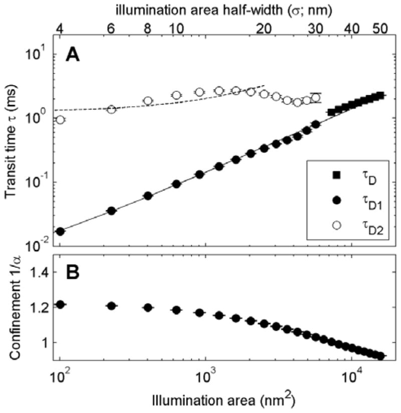
(A) Plot of transit times obtained by fitting either Eqn 3 or Eqn 4 to g(τ) tabulated from Ising model simulations conducted at 1.2Tc and ρ=0.16%. g(τ) tabulated using larger illumination areas are well fit with a single transit time (τ_D), while smaller illumination areas are better described using two distinct transit times τ_D1 and τ_D2. (B) Best fit confinement exponents α determined by fitting the same g(τ) in (A) to Eqn 5. Curves suggest greater confinement (1/α) is apparent at smaller illumination areas. Plots compare qualitatively to Figure 3 in [18].

DISCUSSION

This study of spot size dependent FCS in the 2D Ising model is motivated by the application of these methods to study the motions of fluorescently tagged proteins and lipids in membranes. Nearly always, experimental results of these studies are interpreted as providing information regarding the mobility of single molecules. While this may be the case for some subset of experimental conditions and analysis methods, these correlation methods are also sensitive to time dependent changes in the average concentration. One goal of this study is to demonstrate a range of conditions where it is not appropriate to interpret experimental results in this way, taking advantage of the slow dynamics of average composition in the nearly critical 2D Ising model. In this case, a conventional svFCS analysis suggests the presence of highly anomalous mobility when interpreted as solely a result of single component dynamics, even though single component diffusion is Brownian or nearly Brownian under these conditions. The apparent anomaly occurs because measured FCS curves contain information both on the fast dynamics of single components and the slow dynamics of average composition fluctuations.

Typically, experimental svFCS measurements conducted using a confocal microscope is done at low tracer densities in order to increase sensitivity [15, 16, 18, 20, 32]. The lowest tracer densities explored in the current study was 10 components per 400×400 component box. This corresponds to roughly 15 components per square micron using the calibration of 2 nm per pixel, and only subtle anomalies were observed for this condition. svFCS measurements are also accomplished experimentally using images acquired in wide-field microscopy measurements (e.g. [9, 21, 37]), and these samples are typically more densely labeled. We predict that these measurements are more likely to be subject to interpretation artifacts arising from alternate dynamics of the average composition because of this elevated labeling density. We note that the actual tracer densities presented in this study are arbitrary for several reasons. First, since the 2D ising model is only a coarse grain description of a membrane, single pixels likely do not accurately represent single components. Also, the impact of density on this effect will depend on the detailed dynamics governing structure present in the average composition. In a biological membrane, slow dynamics of the average composition of membrane components could come about from a range of different physical or biological processes in addition to the fluctuations described here. These could include trafficking, electrostatics, membrane curvature, or time dependent protein-protein interactions in signaling processes.

Results presented in Figures 3 and 4 suggest that it may be possible to distinguish effects due to single molecule mobility from those arising from the dynamics of the average composition simply by varying the density of tracers. If results arise entirely from anomalies in single molecule motion, then then they will not depend on density beyond changes in signal to noise, since all components of correlation functions will decrease linearly with increasing density. In contrast, if the apparent anomaly arises from alternate dynamics of the average composition, then results will appear more anomalous with increasing density. This would occur because the amplitude of correlations arising from single molecule motions decreases linearly with increasing density, while the amplitude of correlations arising from the average composition is independent on density. One way that tracer density could be systematically varied could be to utilize light activated fluorescent proteins that are frequently used for super-resolution fluorescence localization imaging in live cells.

Some past work has predicted that the plasma membranes of intact cells resemble a super-critical 2D Ising model like those explored in this study [23–25]. Figure 5 shows that there are conditions where an Ising model can qualitatively mimic results obtained experimentally using svFCS. While this is suggestive, it is not meant to provide experimental support for this theory, and there are important quantitative differences between the findings shown in Figure 5 and those in the experimental membrane literature. One trivial reason for quantitative differences is that we were unable to probe areas larger than 16×10³ nm² (σ=50nm) due to technical limitations. For larger illumination areas, correlation-times begin to exceed reasonable simulation time-scales even for Brownian diffusion. The longest simulations conducted in the current study extended to the equivalent of ~1s (10⁶ updates) making it difficult to sample correlation functions for slow correlation times with the statistics needed to accurately sample g(τ). If larger illumination areas were accessible in these studies, as is routinely accomplished in experiments, we would expect to observe a similar cross-over behavior at larger illumination areas in simulations conducted at lower temperatures.

There are also more fundamental reasons to expect quantitative differences between the current 2D Ising model simulations and experimental results, even if similar physical mechanisms are present in both systems. For one, it has been shown both theoretically and experimentally that the simple diffusive dynamics implemented here do not properly describe the dynamics of composition fluctuations even in simple model membranes [38–40]. This is because hydrodynamics plays important roles in these dynamics, decreasing correlation times most significantly for larger fluctuations. In addition, the dynamics of the average composition is directly linked to the dynamics of single pixels, since these are the only components in these simulations. In a more compositionally complex membrane this need not be the case. This is because different lipids and proteins can have varying single molecule mobility while they collectively contribute to generate the dynamics of the average composition.

In conclusion, here we demonstrate an example where svFCS measurements detect dynamics on multiple time-scales in simulations of the 2D Ising model. In this case, the fast time-scale corresponds to single component diffusive dynamics, the slow time-scale reflects the dynamics of the average composition, and the relative amplitudes of these two contributions vary with both illumination area and tracer density. If acquired g(τ) curves are interpreted as only reflecting single molecule mobility, then one would incorrectly conclude that two diffusing species are present, or that a single diffusive species exhibits confined motions. In actually, single component diffusion is only weakly affected by the presence of heterogeneity in this system, and these apparent anomalies arise due to the presence of slowly varying correlations in the average concentration. We propose that varying tracer density within a single measurement could be used to distinguish anomalous single component mobility from apparent anomalies resulting from the dynamics of the average composition. Overall, these findings emphasize the need to probe complex systems with multiple experimental methods in order to properly interpret experimental findings.

References

- 1.Elson EL. Fluorescence correlation spectroscopy: past, present, future. Biophys J. 2011;101(12):2855–70. doi: 10.1016/j.bpj.2011.11.012. [DOI] [PMC free article] [PubMed] [Google Scholar]
- 2.Ries J, Schwille P. Fluorescence correlation spectroscopy. Bioessays. 2012;34(5):361–8. doi: 10.1002/bies.201100111. [DOI] [PubMed] [Google Scholar]
- 3.Digman MA, Gratton E. Scanning image correlation spectroscopy. Bioessays. 2012;34(5):377–85. doi: 10.1002/bies.201100118. [DOI] [PMC free article] [PubMed] [Google Scholar]
- 4.Kolin DL, Wiseman PW. Advances in image correlation spectroscopy: measuring number densities, aggregation states, and dynamics of fluorescently labeled macromolecules in cells. Cell Biochem Biophys. 2007;49(3):141–64. doi: 10.1007/s12013-007-9000-5. [DOI] [PubMed] [Google Scholar]
- 5.Magde D, Elson EL, Webb WW. Fluorescence correlation spectroscopy. II. An experimental realization. Biopolymers. 1974;13(1):29–61. doi: 10.1002/bip.1974.360130103. [DOI] [PubMed] [Google Scholar]
- 6.Magde D, Webb WW, Elson E. Thermodynamic Fluctuations in a Reacting System - Measurement by Fluorescence Correlation Spectroscopy. Physical Review Letters. 1972;29(11):705. [Google Scholar]
- 7.Schwille P, Korlach J, Webb WW. Fluorescence correlation spectroscopy with single-molecule sensitivity on cell and model membranes. Cytometry. 1999;36(3):176–82. doi: 10.1002/(sici)1097-0320(19990701)36:3<176::aid-cyto5>3.0.co;2-f. [DOI] [PubMed] [Google Scholar]
- 8.Wiseman PW, et al. Two-photon image correlation spectroscopy and image cross-correlation spectroscopy. J Microsc. 2000;200(Pt 1):14–25. doi: 10.1046/j.1365-2818.2000.00736.x. [DOI] [PubMed] [Google Scholar]
- 9.Di Rienzo C, et al. Fast spatiotemporal correlation spectroscopy to determine protein lateral diffusion laws in live cell membranes. Proc Natl Acad Sci U S A. 2013;110(30):12307–12. doi: 10.1073/pnas.1222097110. [DOI] [PMC free article] [PubMed] [Google Scholar]
- 10.Digman MA, et al. Measuring fast dynamics in solutions and cells with a laser scanning microscope. Biophys J. 2005;89(2):1317–27. doi: 10.1529/biophysj.105.062836. [DOI] [PMC free article] [PubMed] [Google Scholar]
- 11.Comeau JW, Kolin DL, Wiseman PW. Accurate measurements of protein interactions in cells via improved spatial image cross-correlation spectroscopy. Mol Biosyst. 2008;4(6):672–85. doi: 10.1039/b719826d. [DOI] [PubMed] [Google Scholar]
- 12.Stone MB, Veatch SL. Steady-state cross-correlations for live two-colour super-resolution localization data sets. Nat Commun. 2015;6:7347. doi: 10.1038/ncomms8347. [DOI] [PMC free article] [PubMed] [Google Scholar]
- 13.Garcia-Saez AJ, Schwille P. Fluorescence correlation spectroscopy for the study of membrane dynamics and protein/lipid interactions. Methods. 2008;46(2):116–22. doi: 10.1016/j.ymeth.2008.06.011. [DOI] [PubMed] [Google Scholar]
- 14.Winckler P, et al. Microfluidity mapping using fluorescence correlation spectroscopy: a new way to investigate plasma membrane microorganization of living cells. Biochim Biophys Acta. 2012;1818(11):2477–85. doi: 10.1016/j.bbamem.2012.05.018. [DOI] [PubMed] [Google Scholar]
- 15.He HT, Marguet D. Detecting nanodomains in living cell membrane by fluorescence correlation spectroscopy. Annu Rev Phys Chem. 2011;62:417–36. doi: 10.1146/annurev-physchem-032210-103402. [DOI] [PubMed] [Google Scholar]
- 16.Wawrezinieck L, et al. Fluorescence correlation spectroscopy diffusion laws to probe the submicron cell membrane organization. Biophys J. 2005;89(6):4029–42. doi: 10.1529/biophysj.105.067959. [DOI] [PMC free article] [PubMed] [Google Scholar]
- 17.Billaudeau C, et al. Probing the plasma membrane organization in living cells by spot variation fluorescence correlation spectroscopy. Methods Enzymol. 2013;519:277–302. doi: 10.1016/B978-0-12-405539-1.00010-5. [DOI] [PubMed] [Google Scholar]
- 18.Eggeling C, et al. Direct observation of the nanoscale dynamics of membrane lipids in a living cell. Nature. 2009;457(7233):1159–62. doi: 10.1038/nature07596. [DOI] [PubMed] [Google Scholar]
- 19.Ruprecht V, et al. Spot variation fluorescence correlation spectroscopy allows for superresolution chronoscopy of confinement times in membranes. Biophysical journal. 2011;100(11):2839–2845. doi: 10.1016/j.bpj.2011.04.035. [DOI] [PMC free article] [PubMed] [Google Scholar]
- 20.Lasserre R, et al. Raft nanodomains contribute to Akt/PKB plasma membrane recruitment and activation. Nat Chem Biol. 2008;4(9):538–47. doi: 10.1038/nchembio.103. [DOI] [PubMed] [Google Scholar]
- 21.Huang H, et al. Effect of receptor dimerization on membrane lipid raft structure continuously quantified on single cells by camera based fluorescence correlation spectroscopy. PLoS One. 2015;10(3):e0121777. doi: 10.1371/journal.pone.0121777. [DOI] [PMC free article] [PubMed] [Google Scholar]
- 22.Honerkamp-Smith AR, et al. Line tensions, correlation lengths, and critical exponents in lipid membranes near critical points. Biophys J. 2008;95(1):236–46. doi: 10.1529/biophysj.107.128421. [DOI] [PMC free article] [PubMed] [Google Scholar]
- 23.Veatch SL, et al. Critical fluctuations in plasma membrane vesicles. ACS Chem Biol. 2008;3(5):287–93. doi: 10.1021/cb800012x. [DOI] [PubMed] [Google Scholar]
- 24.Machta Benjamin B, et al. Minimal Model of Plasma Membrane Heterogeneity Requires Coupling Cortical Actin to Criticality. Biophysical Journal. 2011;100(7):1668–1677. doi: 10.1016/j.bpj.2011.02.029. [DOI] [PMC free article] [PubMed] [Google Scholar]
- 25.Zhao J, Wu J, Veatch SL. Adhesion stabilizes robust lipid heterogeneity in supercritical membranes at physiological temperature. Biophys J. 2013;104(4):825–34. doi: 10.1016/j.bpj.2012.12.047. [DOI] [PMC free article] [PubMed] [Google Scholar]
- 26.Binder K, et al. Interdiffusion in Critical Binary Mixtures by Molecular Dynamics Simulation. Diffusion Fundamentals. 2007;6(10):1–12. [Google Scholar]
- 27.McConnell H. Single molecule diffusion in critical lipid bilayers. J Chem Phys. 2012;137(21):215104. doi: 10.1063/1.4768956. [DOI] [PubMed] [Google Scholar]
- 28.Kawasaki K. Diffusion Constants near Critical Point for Time-Dependent Ising Models. 3. Self-Diffusion Constant. Physical Review. 1966;150(1):285. [Google Scholar]
- 29.Hohenberg PC, Halperin BI. Theory of Dynamic Critical Phenomena. Reviews of Modern Physics. 1977;49(3):435–479. [Google Scholar]
- 30.Sethna JP. Oxford master series in statistical, computational, and theoretical physics. Oxford ; New York: Oxford University Press; 2006. Statistical mechanics : entropy, order parameters, and complexity; p. xix.p. 349. [Google Scholar]
- 31.Kawasaki K. Diffusion Constants near Critical Point for Time-Dependent Ising Models. I. Physical Review. 1966;145(1):224. [Google Scholar]
- 32.Mueller V, et al. STED nanoscopy reveals molecular details of cholesterol- and cytoskeleton-modulated lipid interactions in living cells. Biophys J. 2011;101(7):1651–60. doi: 10.1016/j.bpj.2011.09.006. [DOI] [PMC free article] [PubMed] [Google Scholar]
- 33.Murase K, et al. Ultrafine membrane compartments for molecular diffusion as revealed by single molecule techniques. Biophys J. 2004;86(6):4075–93. doi: 10.1529/biophysj.103.035717. [DOI] [PMC free article] [PubMed] [Google Scholar]
- 34.Morone N, et al. Three-dimensional reconstruction of the membrane skeleton at the plasma membrane interface by electron tomography. J Cell Biol. 2006;174(6):851–62. doi: 10.1083/jcb.200606007. [DOI] [PMC free article] [PubMed] [Google Scholar]
- 35.Edwald E, et al. Oxygen depletion speeds and simplifies diffusion in HeLa cells. Biophys J. 2014;107(8):1873–84. doi: 10.1016/j.bpj.2014.08.023. [DOI] [PMC free article] [PubMed] [Google Scholar]
- 36.Haustein E, Schwille P. Fluorescence correlation spectroscopy: novel variations of an established technique. Annu Rev Biophys Biomol Struct. 2007;36:151–69. doi: 10.1146/annurev.biophys.36.040306.132612. [DOI] [PubMed] [Google Scholar]
- 37.Bag N, Huang S, Wohland T. Plasma Membrane Organization of Epidermal Growth Factor Receptor in Resting and Ligand-Bound States. Biophys J. 2015;109(9):1925–36. doi: 10.1016/j.bpj.2015.09.007. [DOI] [PMC free article] [PubMed] [Google Scholar]
- 38.Honerkamp-Smith AR, Machta BB, Keller SL. Experimental observations of dynamic critical phenomena in a lipid membrane. Physical Review Letters. 2012;108(26):265702. doi: 10.1103/PhysRevLett.108.265702. [DOI] [PMC free article] [PubMed] [Google Scholar]
- 39.Haataja M. Critical dynamics in multicomponent lipid membranes. Phys Rev E Stat Nonlin Soft Matter Phys. 2009;80(2 Pt 1):020902. doi: 10.1103/PhysRevE.80.020902. [DOI] [PubMed] [Google Scholar]
- 40.Inaura K, Fujitani Y. Concentration Fluctuation in a Two-Component Fluid Membrane Surrounded with Three-Dimensional Fluids. Journal of the Physical Society of Japan. 2008;77(11) [Google Scholar]