Large-Scale Multiple Sequence Alignment and Tree Estimation Using SATé

Abstract

SATé is a method for estimating multiple sequence alignments and trees that has been shown to produce highly accurate results for datasets with large numbers of sequences. Running SATé using its default settings is very simple, but improved accuracy can be obtained by modifying its algorithmic parameters. We provide a detailed introduction to the algorithmic approach used by SATé, and instructions for running a SATé analysis using the GUI under default settings. We also provide a discussion of how to modify these settings to obtain improved results, and how to use SATé in a phylogenetic analysis pipeline.

1 Introduction

A typical phylogenetic study estimates a multiple sequence alignment (MSA) from biomolecular sequence data, and then infers a phylogeny using the MSA [1]. While much has been established about the relative performance of phylogeny estimation methods and the importance of picking a highly accurate estimation method, only in recent years has there been substantial study of the impact of the alignment method on the final phylogenetic estimation. It is now understood that the accuracy of the inferred phylogeny depends on the accuracy of the multiple sequence alignments estimated in the preceding phase [2–9], and that inaccurate multiple sequence alignments tend to produce inaccurate trees. While data-sets with low enough rates of evolution can be aligned well using existing fast alignment methods (such as ClustalW [10], Muscle [11, 12], and MAFFT [13]), alignments of datasets that evolve more quickly are substantially harder to estimate, and standard methods typically produce poor alignments on these datasets [3, 4, 14]. Furthermore, many of the highly accurate alignment methods cannot be run on datasets with many sequences, due to computational requirements (running time or memory), and these issues are all particularly challenging for very large datasets with upwards of 5,000 sequences [3, 14]. Thus, the standard two-phase approach to phylogeny estimation is limited by the alignment estimation step, at least for large datasets.

To improve the quality of both the inferred MSA and phylogeny in comparison to the traditional “two-phase” approach (first align, then estimate the tree), methods for simultaneous inference of alignments and phylogenies have been proposed [15–21]. Some of these methods are extensions of maximum parsimony to minimize the total “treelength,” taking both number of substitutions and number of gap events into account; while POY [15] is the most popular of these methods, the accuracy of trees estimated using POY is substantially debated [16, 17]. Co-estimation methods based on statistical models of evolution that include gap events as well as substitutions have also been developed [18–21], of which BAli-Phy [18] is probably the most used and most scalable. Statistical co-estimation methods have the potential to be much more accurate than two-phase methods, because the standard treatment of gaps as missing data in phylogenetic analysis can be statistically inconsistent, even given the true alignment [22]. Statistical co-estimation methods have the potential to be much more accurate than two-phase methods, because the standard treatment of gaps as missing data in phylogenetic analysis can be statistically inconsistent, even given the true alignment [74]. However, not even BAli-Phy is able to run on datasets with more than about 200 sequences.

SATé (an acronym for “Simultaneous Alignment and Tree estimation”) was developed [23] to address the need for highly accurate alignment estimation on datasets with more than a few hundred sequences. SATé uses an iterative technique in which each iteration computes an alignment (using a divide-and-conquer strategy that estimates alignments on subsets and then merges the subset alignments) and then computes a tree for that alignment using maximum likelihood heuristics. SATé produces highly accurate alignments and trees in no more than 24 h, even on datasets with 1,000 sequences. A modification to the divide-and-conquer strategy led to a substantially improved version, called SATé-II, that achieves even better accuracy in less time [24]. Finally, while both versions of SATé were studied using RAxML [25] for the maximum likelihood tree estimator, the use of FastTree [26] led to additional speed-ups and comparable alignment accuracy (unpublished data). We also extended SATé by adding other techniques for estimating alignments on subsets and/or merging subset alignments [27, 28]. This new version of SATé is available in the public distribution, and is able to analyze datasets that were too large for the original version. Most importantly, on large datasets (with 500 or more sequences), especially those that evolve quickly, SATé can provide much more accurate alignments and trees than other methods. SATé has been used to analyze protein as well as nucleotide datasets for many different types of organisms (birds, plants, bacteria, etc.). Many of these analyses have been on small datasets, with less than 100 sequences; however, SATé has also been used to analyze almost 28,000 rRNA sequences, spanning the domains of Archaea, Bacteria, and Eukaryota [24].

Although the first publication [23] of SATé has been cited over 100 times, the current implementation in the public distribution (available from the University of Kansas Web site at http://phylo.bio.ku.edu/software/sate/sate.html) is based on the second publication [24]. The focus of this chapter, therefore, is on the new implementation of SATé. We limit our discussion to the GUI usage, but readers interested in command-line usage can obtain additional information from the tutorial available online from the Kansas Web site (see ^{Note 1}), or from the SATé user group (see ^{Note 2}). SATé is under active development, with extensions to handling fragmentary data (as created by next generation sequencing technologies), improved analysis of protein sequences, etc., and users may wish to contact the UT-Austin SATé group for information about these plans, or to suggest new developments (see ^{Note 3}). Finally, phylogenetic estimation is a large and complex research discipline, and we direct the interested reader to [29] for a more in-depth discussion.

2 SATé Design Goals and Limitations

SATé was designed to enable fast and accurate estimation of alignments and trees for nucleotide datasets with hundreds to thousands of sequences [23, 24]. Its design, which is based on divide-and-conquer, improves accuracy on those datasets for which the best alignment methods cannot run due to computational requirements (either memory or time). Therefore, SATé is not designed to improve accuracy on those datasets that are small enough to be handled well by standard methods. In addition, although SATé is designed for large datasets, the largest dataset ever analyzed by SATé is the 16S.B.ALL dataset with 27,643 rRNA sequences with 6,857 sites [23], and we do not know how well it will scale for very large datasets with many tens of thousands of sequences.

Some datasets fall clearly outside of the design goals of SATé. SATé is also not designed for alignment estimation of datasets that are extremely long (hundreds of thousands of nucleotides) or that evolve with rearrangements rather than just indels (insertions and deletions) and substitutions; thus, whole genome alignment [30] is not part of SATé’s capabilities. SATé has also not been designed for datasets with substantial missing data or fragmentary data from short read sequencing projects. Phylogeny estimation for highly fragmentary data can be obtained through methods based on “phylogenetic placement” [31–33]. Multiple sequence alignment estimation for highly fragmentary data can also be addressed through these phylogenetic placement methods, but has not been sufficiently studied in this context.

3 Algorithm

SATé uses iteration to produce improved alignments and trees, so that each iteration uses the results from the previous iteration to start its analysis, and then reestimates a multiple sequence alignment and tree for the dataset. Empirically, our studies have shown that the iterations quickly converge to good alignments and trees, with the biggest improvement occurring in the first iteration. Therefore, even a single iteration can result in an improved tree and alignment, and several iterations provide increased accuracy.

The studies in [3, 14] showed that the most accurate alignment methods (such as MAFFT, in its most accurate setting) could not be run on datasets with thousands of sequences, and that all methods have reduced accuracy for large enough rates of evolution and numbers of sequences. SATé overcomes this barrier using divide-and-conquer. It divides an input sequence dataset into subsets that are small enough that highly accurate alignment methods can be run on them, thus producing “subset alignments”. SATé then merges the subset alignments together to produce an alignment of the full dataset, on which a tree can then be estimated using maximum likelihood methods. By repeating this process several times, the alignments and trees become increasingly accurate.

By design, SATé has several algorithmic parameters that determine how it runs. These have default values, but can also be reset by the user. Understanding the algorithmic parameters is helpful to obtaining improved accuracy for dataset analyses. Here we describe the algorithmic structure, and point out the algorithmic parameters that the user can set.

The input to SATé is a set of unaligned sequences. However, the user can also provide an initial alignment and/or tree, which can then be used by SATé to begin the iterative process. If none are provided, then SATé will estimate its own alignment and tree for the input sequences.

The main analysis then proceeds by repeating the following steps in an iterative fashion. The tree T from the previous iteration is used to guide the divide-and-conquer strategy for the current iteration. The tree itself is estimated using maximum likelihood (either using RAxML or FastTree) on the alignment on the sequences, and so has branch “lengths” (indicating substitution parameters for the Markov model of evolution). A branch e is selected in the tree T (either the “centroid” branch, which divides the tree into two subtrees with roughly equal numbers of taxa, or the “longest” branch). When this branch is removed from T, it divides the leaves of T into two subtrees. This decomposition is repeated until every subtree has a small enough number of leaves, as determined by the “maximum subproblem” size provided by the user (this is one of the algorithmic parameters). Once every subtree is small enough, the decomposition ceases, and each of these subtrees defines a “subproblem” of sequences (associated to the leaves of the subtree). The sequences in each subproblem are realigned using a multiple sequence alignment method selected by the user (the “aligner”), and the resulting subset alignments are then merged into an alignment on the full set of sequences. This merger step is handled by repeatedly applying an alignment “merger” method (also specified by the user) in the reverse order of the decomposition. Finally, a phylogenetic tree is estimated using either RAxML or FastTree.

Each iteration of SATé produces an alignment and tree, and thus each SATé analysis produces a sequence of alignment/tree pairs (one pair per iteration). Each alignment/tree pair has a maximum likelihood (ML) score as well, which can help the user to select a tree and alignment from the sequence of alignment/tree pairs. SATé terminates the iterative process based on a user-specified termination condition, which can be either elapsed wall-clock time, or a maximum number of iterations, or a lack of improvement in ML score. The final alignment/tree pair output by SATé is chosen from among the sequence of alignment/tree pairs generated during the course of analysis, and can be the pair with the best maximum likelihood score or the final pair produced by SATé.

4 Algorithmic Parameters and Software Settings

The SATé algorithm specifies several algorithmic parameters, and can be adapted to the needs of a particular dataset analysis by changing these parameters. However, it can also be run in default mode, so that the user does not need to set any parameters.

The software implementation of the SATé algorithm provides user-selectable settings for each of the algorithmic parameters. Table 1 describes the relationship between the algorithmic parameters and software settings; additional discussion of these parameters (and guidance on how to set these parameters for improved performance) is provided in the text.

Table 1.

Relationship between algorithmic parameters and software settings

Algorithmic parameter	Software setting	Software setting choices	Description
Subproblem alignment method	“Aligner” dropbox	MAFFT, ClustalW, Prank [26], Opal [27]	This determines the method used to align the subsets of the sequences, and the default is MAFFT
Alignment merge method	“Merger” dropbox	Muscle, Opal	This determines how subset alignments are merged together. Muscle is the default, but Opal should be used if the dataset is small enough
ML-based phylogenetic estimation method	“Tree Estimator” dropbox	FastTree, RAxML	This determines how phylogenetic trees are estimated in each iteration; the default is FastTree, due to its improved speed relative to RAxML
Substitution model	“Model” dropbox	Many models, depending on type of data and ML tree estimation method	The model selected determines the parameters optimized by the ML tree estimation method. See [29]
Maximum subproblem size	“Max. Subproblem” dialog	Percentage (1–50 %), size (1–200)	This determines the maximum size subset given to the “aligner” method
Decomposition edge	“Decomposition” dropbox	Centroid, longest	This determines the edge used to decompose the dataset into subsets. The default setting is the centroid edge
Termination condition	“Apply Stop Rule” dropbox	After Last Improvement, After Launch	This determines when the stopping rule is evaluated. We recommend using “After Last Improvement” unless your dataset is very large
Termination condition	“Stopping Rule” dialog -“Blind Mode Enabled” checkbox	Checked/unchecked	This determines which tree (best ML or current tree) is used in the subsequent iteration
Termination condition	“Stopping Rule” dialog -“Time Limit (hr)” dialog/”Iteration Limit” dialog	0.01–72 h (“Time Limit (hr)” dialog) 1+ (“Iteration Limit” dialog)	This determines whether time or number of iterations is used to define when SATé stops
Final tree/alignment pair output by SATé	“Return” dropbox	Best, Final	This determines which tree and alignment pair (Best ML or last pair computed) is output
Parallelization	“CPU(s) Available”	1–16	This determines whether SATé will be run in parallel mode
Multi-gene analysis	“Multi-Locus Data” checkbox/”Sequence files” button	Checked/unchecked Folder dialog box	This enables a multi-gene analysis. See the “Advanced Analysis” section
Miscellaneous algorithmic modifications	“Extra RAxML Search” checkbox	Checked/unchecked	Checking this makes SATé perform a RAxML analysis of the final alignment
Miscellaneous algorithmic modifications	“Two-Phase (not SATe)” checkbox	Checked/unchecked	Check to run a two-phase analysis (first align and then compute an ML tree)

Choosing one of the settings in the “Quick Set” dropbox will automatically configure the software settings to perform one of the SATé-II analyses described in ref. 23. Subsequent modifications to software settings will cause the “Quick Set” dropbox to display the “(Custom)” choice

After loading the input files in the SATé program, the software provides the option to automatically select all software settings based upon the properties of the input dataset. The following sections cover this usage scenario first, and we recommend the automatically selected settings unless more advanced analyses are required. Advanced usage scenarios involving changes to the automatically selected software settings are discussed later in this chapter.

5 Additional Guidelines for Selecting Algorithmic Parameters

“Aligner” method

The choice of method to align the subsets has a large impact on the resultant alignment and tree. The default is MAFFT, due to its high accuracy on both simulated and biological data on both nucleotides and amino acid datasets [2, 3, 13, 14, 23, 24]. However, Prank has also been used in studies [24], and has the advantage over MAFFT and other standard alignment methods of not “over-aligning” as much. Because Prank is slower than MAFFT, the use of Prank to align subsets should be accompanied by a reduction in the maximum subset size so that the runs can complete. Finally, Opal and ClustalW are also enabled. Opal presents memory challenges on large datasets, and is not recommended unless the dataset is small enough. ClustalW is fast and can be used on any dataset size, but may not provide the same accuracy as MAFFT.

“Merger” method

Only Muscle and Opal are enabled for merging alignments. Muscle is the current default, because it has low memory requirements while Opal has high memory requirements. However, we strongly recommend Opal because it generally produces more accurate alignments. Therefore, we recommend using Opal unless you do not have sufficient memory for your dataset analysis. However, this is unlikely to be a problem except for very large datasets (with more than 10,000 sequences), if you have a reasonable amount of memory on your laptop or desktop machine.

“Tree Estimator” method

Only RAxML and FastTree are enabled for estimating trees from alignments, and FastTree is the default. Both are heuristics for maximum likelihood, which is a computationally hard problem. FastTree is much faster than RAxML, and generally produces trees of very similar accuracy [34]. Furthermore, in our unpublished studies, the use of FastTree instead of RAxML within SATé produces alignments of comparable accuracy and only a small decrease in accuracy for the trees. Because of its great speed advantage, however, we recommend the use of Fast-Tree. If FastTree is used, a final RAxML run can be applied to the output alignment in order to obtain a RAxML tree (and thus potentially improved accuracy).

Substitution model

This refers to the statistical model [29] used by the maximum likelihood method (RAxML or FastTree) to estimate trees from alignments. The choice of statistical model depends on whether your data are nucleotide or amino-acid sequences, and also on whether you are using RAxML or FastTree as the tree estimator, since these enable somewhat different models. For nucleotide data, the default using RAxML is GTRCAT, while the default using FastTree is GTR + G20. GTR stands for the General Time Reversible (GTR) model, which is the most general substitution model available within SATé. G20 and CAT refer to how the model handles the Gamma rates-across-sites model; G20 is the GAMMA distribution approximated by 20 rate categories, while CAT [35] is a heuristic approximation to the GAMMA rate-variation model. Alternative settings for RAxML include GTRGAMMA (GTR + GAMMA) and GTRGAMMAI (GTR + Gamma + Invariable). Alternative settings for FastTree include JC (the Jukes-Cantor model) [36] instead of GTR, but this simplified model is not recommended except under very unusual circumstances where the data seem to fit the Jukes-Cantor model best (unlikely for most data). Note that the GAMMA setting is usually used in phylogenetic analyses, but the CAT setting improves speed at a potential loss of phylogenetic accuracy. For amino-acid datasets, the choice of substitution model is more complicated; see the section below on Amino-Acid Datasets for more information.

Maximum subproblem size

This is the maximum allowed size of the subsets of sequences, and so determines how many times the decomposition strategy is applied. The default depends on the dataset size (and will be set by SATé after you input your data). However, the main issue in setting the maximum subproblem size is the method used to align subsets. When MAFFT is the aligner method, then keeping the maximum subproblem size to at most 200 allows the most accurate version of MAFFT (L-INS-i) to be used to align the subsets, and this results in the best accuracy. If you wish to use Prank instead of MAFFT to align subsets, the maximum subproblem size should be reduced substantially, because Prank is computationally more expensive. Similarly, the use of Opal to align subsets will require a reduction in subproblem size because of Opal’s memory requirements (and hence increased running time). Less is known about how to set the maximum subproblem size when ClustalW is used for aligning subsets, but the default settings are probably fine.

Decomposition edge

This algorithmic parameter determines how the dataset is decomposed—through the centroid edge (which produces a roughly equal decomposition into two datasets) or the longest branch. The default is the centroid edge, and this produces results of similar accuracy to the longest edge, while being much faster.

Stopping rule

There are various settings that determine the stopping condition and when it is evaluated. You can set the stopping rule to be defined by the number of iterations or time, and at least one of these must be specified (selecting both means that either can trigger the stopping rule). You can begin this stopping rule immediately (“After Launch”) or only after the ML score stops improving (“After Last Improvement”). We recommend using “After Last Improvement” unless your dataset is so large that you need to limit the number of iterations. “Blind mode” means that the previous iteration’s tree will always be used as the tree in the beginning of the next iteration, regardless of its ML score. Disabling “blind mode” means that the best-scoring tree so far will be used in the beginning of the next iteration, which can cause the iterative search to become stuck in local optima. We recommend enabling “blind mode”.

Final tree/alignment

This determines which tree is the output for the SATé run. The “Best” setting returns the best-scoring alignment/tree pair encountered during the SATé analysis. The “Final” setting returns the final alignment/tree pair from SATé.

CPUs available

This is the number of CPUs in your machine that SATé should use, and using multiple CPUs can speed up the analysis. However, do not set this number to more CPUs than you have! See ^{Note 4}.

Extra RAxML search

Checking this box makes SATé perform a RAxML analysis of the final alignment. If time is not highly constrained (and your dataset is not too large), checking this box is recommended if you have used FastTree for the ML tree estimator. However, when you use RAxML for the ML tree estimator, it automatically computes a RAxML tree on the final alignment, and so it does not make any sense to check this box.

Two-phase (not SATé)

Check this box to run a two-phase analysis (first align and then compute an ML tree) using the settings in the “External Tools” window, instead of running a SATé analysis. This may not produce alignments and trees as accurate as those produced by SATé, but should be faster.

6 Advanced Topics

Amino-acid datasets

The analysis of amino-acid datasets presents some additional challenges and opportunities. Compared to nucleotide sequences, the selection of the substitution model is more complicated, since the models are not “nested”. The best model for your data needs to be selected using a statistical test [37, 38], however, JTT [39] and WAG [40] models are often used for amino acid datasets and are reasonable defaults. The models available for use for amino-acid analyses are displayed within SATé after you check the box indicating that your data are proteins, and depend upon the ML method you have selected (RAxML or FastTree). RAxML enables many more models than FastTree, and so may be preferable. The other amino-acid models available in SATé when used with RAxML are DAYHOFF [41], DCMUT [42], MTREV [43], RTREV [44], CPREV [45], VT [46], BLOSUM62 [47], MTMAM [48], and LG [49], each in combination with a rates-across-sites model. To set base frequencies for these amino-acid models to empirical base frequencies, add an “F” suffix to the name of the model; see the RAxML documentation for details (available from http://sco.h-its.org/exelixis/old-Page/RAxML-Manual.7.0.4.pdf). SATé has been used to analyze protein datasets [50, 51], but we have not studied SATé as a protein aligner nearly as thoroughly as we have studied it as a nucleotide sequence aligner; therefore, the default settings for the algorithmic parameters may not be optimized well. Finally, amino-acid alignment estimation in particular can be enhanced with structural (secondary or tertiary) information about the proteins, information that the aligner methods (MAFFT, ClustalW, Prank, and Opal) used by SATé do not use. Therefore, there is the potential for improved accuracy to be obtained through the use of a different set of protein alignment methods, including methods such as SATCHMO-JS [52] that employ Hidden Markov Models to take advantage of particular properties of protein alignments.

Large datasets

We now present guidelines for the analysis of data-sets with 1,000 or more sequences. However, because SATé has not been tested on datasets with more than 28,000 sequences, our recommendation on very large datasets should be taken as our best guess, at this time, for how to handle such datasets. We strongly recommend the use of FastTree rather than RAxML for ML tree estimation in each iteration: FastTree is much faster than RAxML, and our preliminary studies (unpublished) suggest that using FastTree instead of RAxML produces the same quality alignments in a fraction of the time. However, switching to FastTree can reduce the tree accuracy slightly, and so the user may wish to use RAxML on the final alignment returned by SATé. For very large datasets, the final RAxML analysis could take a long time, and so an alternative is to run SATé using FastTree and without any final RAxML run, save the resultant alignment and tree, and then run RAxML on the final alignment. We recommend using MAFFT for aligning subsets, using a maximum alignment subset size of 200, and the centroid edge decomposition. We recommend using Opal to merge subset alignments instead of Muscle, unless the dataset is so large (in number of sequences and/or sequence length) that the memory requirements for using Opal exceed what you have available on your machine. Opal should never be used as the subset alignment technique on extremely large datasets (its memory requirements will slow down the analysis dramatically). Prank is too slow to use on even moderately large datasets, and therefore Prank should not be used as the subset aligner. The use of ClustalW for the subset aligner will not cause running time issues, but there is little evidence that ClustalW is likely to produce more accurate alignments than MAFFT; therefore, it is not recommended as a subset aligner.

For very large datasets, providing an initial alignment (and possibly initial tree) to SATé can speed up and potentially improve the analysis. If you run SATé without providing it an initial alignment and/or tree, this initial alignment will be estimated using MAFFT, which is run in its less accurate setting (in extreme cases, this will be MAFFT-PartTree [53]) on very large datasets. However, faster and potentially more accurate estimations of initial alignments might be achievable using other methods, such as Clustal-Omega [54] for amino-acid sequences or MAFFT-profile [55] for nucleotide sequences. Once the initial alignment is provided, SATé will use FastTree to estimate the initial tree on the alignment. Because SATé is quite robust to its initial tree [23, 24], this means that the initial alignment need not be particularly accurate. The analysis of very large datasets presents both memory and running time challenges; see ^{Notes 5–7} for advice on how to handle problems that may arise.

Small datasets

Using SATé to estimate trees and alignments on very small datasets (with less than 200 sequences) may not result in improved accuracy, since these datasets can be analyzed well using methods such as MAFFT; however, datasets of this size have been analyzed using SATé (see, for example, [50, 51, 56–58]).The main recommendation we make for the analysis of small datasets is to use 50 % as the maximum subproblem size, rather than a smaller percentage, and to otherwise use the standard defaults. In addition, for small enough datasets, phylogeny estimation methods that are generally too computationally intensive to use on even moderately large datasets (such as MrBayes [59]) can be used to estimate a tree on the resultant SATé alignment.

Exploring the solution space

One of the appealing aspects of SATé is that it provide opportunities for exploration of the set of alignments and trees that are returned during the SATé run, which can allow you to explore how alignments impact the tree estimation, among other things. This is particularly useful on small datasets because each iteration can be done quickly, and so many iterations can be run on small datasets. To enable this exploration, we recommend setting the stopping rule to an iteration limit, and setting that limit to a large number (how large, of course, depends upon how much time you wish to devote). There are many methods for exploring sets of trees [60–64], each aimed at extracting different types of information. Similar analyses for exploring sets of alignments are not yet in standard use, but pairs of alignments are often compared to determine common homologies [65].

Multi-locus datasets

Often the objective is the estimation of a species tree from a set of different genes, each of which involves an alignment and tree estimation. You have several options for how to do a multi-locus analysis, depending on whether you are concerned about the potential for gene trees to be different from the species tree. That is, true gene trees can differ from the true species tree due to biological processes such as incomplete lineage sorting, gene duplication and loss, and horizontal gene transfer [66]. Therefore, the choice of how to estimate the species tree from a set of estimated gene trees can take some care. If you have concerns about potential conflict between gene trees, you can run SATé on each marker separately, thus producing independently estimated gene trees and alignments for each gene, and these estimated trees and alignments can then be used to estimate a species tree using techniques that are specifically designed to combine estimated gene trees into a species tree. See [67–74] and references therein for an introduction to methods that can estimate phylogenetic trees and networks in the presence of these processes that cause gene tree incongruence. If you are not concerned about potential gene tree conflict, we recommend using SATé in its default setting for multi-locus datasets. This analysis operates by concatenating the datasets together, and then uses the standard iterative divide-and-conquer strategy to produce alignments of each locus and a tree on the entire dataset.

General advice

We recommend that you back up your files (see ^{Note 8}) for all SATé analyses. This is generally a good practice, but especially for large dataset analyses or when you wish to explore the solution space, which can take a substantial amount of time to run. Some analyses may benefit from the use of archival systems (see ^{Note 9}), especially if your analyses involve very large datasets that you plan to explore in multiple ways.

7 Materials

The following sections pertain to Apple computers running recent versions of the Mac OS X operating system (including versions 10.4, 10.5, 10.6, and 10.7). For alternative operating systems and hardware, please consult the relevant software documentation.

7.1 Software

1. File format conversion software. SATé utilizes FASTA-formatted sequence files and Newick-formatted tree files. Many software packages and Web portals provide a format conversion capability. For example, the European Molecular Biology Open Software Suite (http://emboss.sourceforge.net/) [75] contains a module to convert sequence formats (see instructions for the seqret command at http://emboss.sourceforge.net/docs/themes/SequenceFormats.html). In addition, the savetrees command in PAUP* [76] will output a tree in Newick format when the “FORMAT = PHYLIP” option is specified.

2. SATé software. Available from http://www.cs.utexas.edu/~phylo/software/SATé/ and http://phylo.bio.ku.edu/software/SATé/SATé.html. We used version 2.2.5, although the methodology in this chapter is compatible with any recent version of the SATé software.

7.2 Hardware

1. We recommend using an Apple computer with a recent Intel processor and at least 1 GB of available memory. Large-scale analyses are primarily constrained by memory requirements (see ^{Note 6}). Clock speed and related CPU features primarily affect running time.

2. While the SATé installation requires less than 100 MB of disk space, much more disk space is required for a large-scale analysis, especially if the analysis runs for many iterations over a long period of time (see ^{Note 7}).

8 Methods

8.1 Install Software

1. Download the latest SATé software package from http://phylo.bio.ku.edu/software/SATé/SATé.html. See ^{Note 10} in the event of installation problems.

2. Open the downloaded package file and view its contents (Fig. 1).

3. Create a new folder for the new SATé installation in a separate location on the hard drive (see ^{Note 11}).

4. Drag and drop the package contents to the new folder.

5. In the new folder, double-click the SATé icon to start the SATé program.

Fig. 1.

Contents of the SATé software package. The SATé application is represented by the rightmost icon. The “doc” folder contains software documentation. The “data” folder contains example input files, and the corresponding output files are contained in the “sample-output” folder

8.2 Preparing Input File and Output Folder

1. If the input sequence file is not in FASTA format, use a third-party program to convert the input file to FASTA format. See ^{Note 12}.

2. We recommend that a new output folder be created for each SATé analysis.

8.3 Basic Analysis: Nucleotide Datasets

1. After starting the SATé program, the main analysis window appears (Fig. 2). The default settings correspond to the “SATé-II fast” analysis described in [24], which are appropriate for a wide range of phylogenetic studies. Make sure that the “SATé-II-fast” option is selected in the “Quick Set” drop-down menu.

2. Click the “Sequence file” button to load the input file. Locate and select the FASTA-formatted input file in the dialog box.

3. A dialog box appears with a query about automatic customization of some analysis settings based on the input file (Fig. 3). Click “OK” to enable the automatic customization. Customized settings will be reflected in the “SATé Settings” box of the application.

4. In the “Decomposition” drop-down menu, select “Centroid”. If this changes the current defaults, the “Quick Set” menu will change to the “(Custom)” option.

5. In the “Job Name” field, provide a unique name for the analysis.

6. Click the “Output Dir.” button. Locate and select the desired output folder in the dialog box. If output files for a job with the same name exists in the output folder, the output files of the current analysis will contain an additional integer to prevent file collisions.

7. Press the “Start” button to begin the SATé analysis. As the analysis proceeds, the bottom text window shows progress updates. The time duration required for an analysis depends on many factors, especially dataset size and complexity (see ^{Notes 6} and ⁷).

8. While the analysis is running, the “Start” button is replaced with a “Stop” button. In the event that the analysis needs to be canceled, press the “Stop” button (see ^{Note 6}).

9. Once the message “Job myjob is finished.” appears in the bottom text window (for an analysis named “myjob”), the analysis is complete (Fig. 4).

10. To view the output of the analysis, navigate to the output folder. The output files are described in Table 2.

Fig. 2.

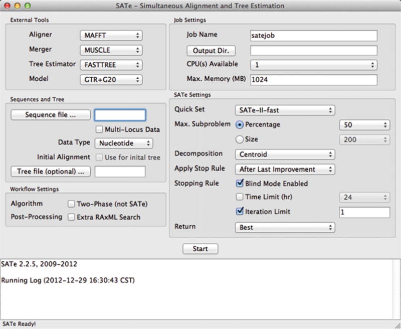
The main SATé application window

Fig. 3.

After pressing the “Sequence file” button and selecting an input file to read, SATé responds with a prompt about automatic configuration. Selecting “OK” will enable automatic configuration of analysis settings based on the input file

Fig. 4.

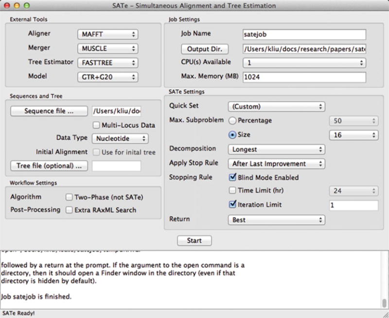
The conclusion of a typical SATé analysis

Table 2.

Output files from a SATé analysis

Output file name	Description
myjob.marker001.sequence.aln	SATé alignment
myjob.tre	SATé tree
myjob.score.txt	ML score for the SATé alignment/tree pair
myjob.out.txt	Diagnostic messages
myjob.err.txt	Error messages. If this file is not empty, check your settings and retry the analysis
myjob_temp_iteration_initialsearch_seq_alignment.txt	Starting alignment
myjob_iteration_initialsearch_tree.tre	Starting tree
myjob_temp_iteration_0_seq_alignment.txt, myjob_temp_iteration_1_seq_alignment.txt, etc.	Intermediate alignments
myjob_iteration_0_tree.tre, myjob_iteration_1_tree.tre, etc.	Intermediate trees
myjob_temp_name_translation.txt	Taxa in intermediate trees and alignments are renamed according to this translation table. The temporary substitute name for a taxon is shown on one line, followed by its original name, and then a blank line

The analysis used a job name of “myjob” and the input file was named “sequence.fasta”

8.4 Basic Analysis: Amino Acid Datasets

1. See ^{Note 3}. Follow the steps listed in the Subheading 8.3, but be sure to pick “Protein” for Data Type (in the Sequences and Tree dialog box). The automatic customization step will configure the settings appropriately (Fig. 5).

Fig. 5.

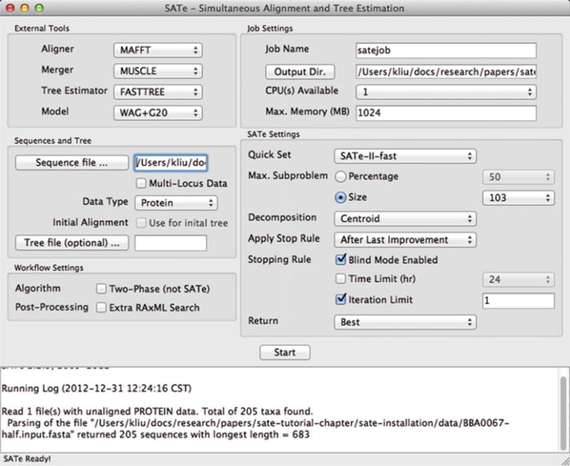
The start of a SATé analysis of an amino acid dataset

8.5 Advanced Analysis: More Iterations Desired

1. If additional time and computational resources are available, an extended, more thorough SATé analysis can be run. To do this, run the following steps.

2. In the “Quick Set” drop-down menu, select the “SATé-II-ML” option.

3. In the “Decomposition” drop-down menu, select the “Centroid” option.

4. Proceed with steps 7 through 10 from the “Basic Analysis” sections 8.3 and 8.4, but be sure to pick a large enough number of iterations.

8.6 Advanced Analysis: Providing an Initial Alignment (and/or Initial Tree)

1. Providing a precomputed alignment and/or tree to SATé can save substantial time. To begin, follow steps 1 through 6 in the “Basic Analysis” sections 8.3 and 8.4. During step 2, provide a FASTA-formatted file with aligned sequences. The “Initial Alignment” dialog will have the “Use for initial tree” checkbox enabled. If a user-specified starting tree is available, click the “Tree file (optional)” button and provide the Newick-formatted starting tree file name.

2. Proceed with steps 7 through 10 from the “Basic Analysis” section.

8.7 Advanced Analysis: Very Large Datasets (More Than 10,000 Sequences)

1. Very large datasets with tens of thousands of sequences or more pose a special computational challenge. Changing software settings is recommended in this instance, although the optimal settings for a particular dataset depend upon many factors. Thus, while we provide specific suggestions for this case, experimenting with software settings is also advisable, with the caveats described in ^{Notes 5} through ⁷. See the discussion above (for “large dataset analyses”) for some explanations for why we make the following recommendations.

2. If an alignment and tree are already available, we recommend providing them to SATé. This recommendation is strongly recommended for very large datasets (with 10,000 sequences or more), but beneficial for all analyses.

3. Otherwise, we recommend computing an initial alignment using either MAFFT’s PartTree algorithm or Clustal Omega; these tools are not available within the GUI usage of SATé, and so this will need to be done offline. For an input file named “sequence.fasta”, the PartTree algorithm can be invoked using the following command: mafft -parttree -retree 2 -partsize 1000 sequence.fasta > startingAlignment.fasta. The command to run Clustal Omega is: clustalo –auto –dealign -i sequence.fasta > startingAlignment.fasta. Once you have the alignment, you can provide this to SATé as the initial alignment (see above).

4. In the “External Tools” window, choose the following software settings: “MAFFT” for the “Aligner” dropbox, “Muscle” for the “Merger” dropbox, and “FastTree” for the “Tree Estimator” dropbox. For nucleotide analyses, select “GTR + CAT” for the “Model” dropbox, and for protein analyses, select JTT + CAT.

5. In the “Sequences and Tree” window, provide your initial alignment (if available), and click on “initial alignment (use for initial tree)”. Follow from step 3 in Subheading 8.6.

6. In Workflow Settings, do not select “Extra RAxML Search”, unless your dataset is not particularly big–the final RAxML search could be the most computationally intensive part of your analysis, and may not provide substantial benefits.

7. In the “Job Settings” window, make sure you provide the number of CPU(s) available (this will have a large impact on the running time, if more than 1 CPU can be used in the analysis). Also make sure that the “Max. Memory (MB)” dialog specifies the correct amount of available memory, since memory limitations are often a problem that cause running times to increase. See ^{Note 7}.

8. In the “SATé settings” window, you can use Quick Set to select “ SATé-II-fast”; this will set all the settings appropriately. Alternatively, you can modify the settings as follows. Select the “Size” radio button in the “Max. Subproblem” field and a size of 200 in the dropdown menu. Set the decomposition to “centroid” (because using “Longest” will not only slow down the analysis, but also should only be run with Opal, and Opal should not be run with large datasets). Set the “Apply Stop Rule” to either “After Launch” (for very large datasets) or to “After Last Improvement”. Do not select “Blind Mode Enabled” if your dataset is very large. It is also probably not a good idea to use a time limit for the stopping rule if your dataset is very large, since it is possible for a single iteration to not complete in the time you pick. Therefore, we recommend instead picking an iteration limit. The number of iterations you pick should depend on your dataset, but for very large datasets, it may be best to have a small number (say, 2) of iterations. If these complete quickly, you can always use the output alignment and tree to initialize another SATé run! We recommend setting “Return” to “Best”.

8.8 Advanced Analysis: Multi-gene Datasets

1. Prepare your dataset by creating a new folder and saving the sequence data for each gene (or marker) in a separate FASTA-formatted file in the new folder. Each FASTA-formatted file name must end with the suffix .fasta or .fas. Make sure that the set of taxon names are identical across all of the FASTA files.

2. Begin by following step 1 from the “Basic Analysis” section.

3. Click the “Multi-Locus Data” checkbox in the “Sequences and Tree” pane. Notice that the “Sequence file” dialog changes into the “Sequence files” dialog. Click the “Sequence files” button and choose the folder containing the input files.

4. Now run the analysis by following steps 3 through 9 in the “Basic Analysis” section.

5. After the analysis finishes, the output files will be saved to the output directory. The file names and descriptions will match Table 2, with one exception. For an analysis with job name “myjob” and input files named “geneA.fasta”, “geneB.fasta”, “geneC.fasta”, and so on, SATé saves the output alignments in files named myjob.marker001.geneA.aln, myjob.marker002. geneB.fasta.aln, myjob.marker003.geneC.fasta.aln, and so on.

9 Summary and Related Work

SATé is a method for large-scale alignment and tree estimation that has been shown to give very good results on both biological and simulated datasets of both nucleotide and amino-acid datasets. However, the reasons for its good performance are subtle: for example, it is not the case that allowing the alignment to change arbitrarily and seeking the alignment with the best maximum likelihood score (treating gaps as missing data) will lead to good trees [75]. Instead, the benefits to using SATé come because alignment methods with great accuracy but poor scalability can be used to estimate alignments on small subsets of the sequence dataset, and the resultant subset alignments can then be merged into an alignment on the full dataset. This design strategy means that SATé can continue to improve in accuracy as new alignment methods are developed. Similarly, as better tree estimation methods are developed (including ones that might use gap events in a more informative manner), SATé can continue to improve in accuracy and/or scalability though the incorporation of these improved methods.

Alternative approaches to large-scale phylogeny estimation that do not require the estimation of a multiple sequence alignment have also been developed; of these, DACTAL [14] has been shown to give results that are almost as accurate as SATé, while being able to run on very large datasets. However, DACTAL is not completely alignment-free; instead, it computes alignments and trees on small subsets (carefully selected from the taxon set), and combines these smaller trees into a tree on the full set of taxa using SuperFine [77–79]. By combining this divide-and-conquer strategy with iteration, it quickly produces highly accurate trees. Truly alignment-free estimation has also been considered [80, 81], with some methods have strong theoretical guarantees [82]. Certainly the benefits of not requiring a full multiple sequence alignment are significant, especially in terms of running time. Ongoing research will show whether methods that do not require full sequence alignments are able to produce trees of comparable accuracy to the best of the tree estimation methods that do (at some point) estimate an alignment on the entire dataset.

This tutorial is limited to the GUI usage of SATé; readers interested in using the command line version are directed to the online tutorial [83]. Datasets and software to study alignment and phylogeny estimation methods are available through the SATé group Webpages at UT-Austin [84]. For additional discussion on methods for phylogenetic analysis, including data selection, see [85, 86].

References

- 1.Kemena C, Notredame C. Upcoming challenges for multiple sequence alignment methods in the high-throughput era. Bioinformatics. 2009;25:2455–2465. doi: 10.1093/bioinformatics/btp452. [DOI] [PMC free article] [PubMed] [Google Scholar]
- 2.Nelesen S, Liu K, Zhao D, et al. The effect of the guide tree on multiple sequence alignments and subsequent phylogenetic analyses. Pac Symp Biocomput. 2008;2008:25–36. doi: 10.1142/9789812776136_0004. [DOI] [PubMed] [Google Scholar]
- 3.Liu K, Linder CR, Warnow T. Multiple sequence alignment: a major challenge to large-scale phylogenetics. PLoS Curr. 2010;2:RRN1198. doi: 10.1371/currents.RRN1198. [DOI] [PMC free article] [PubMed] [Google Scholar]
- 4.Wang L-S, Leebens-Mack J, Wall PK, Beckman K, de Pamphilis CW, Warnow T. The impact of multiple protein sequence alignment on phylogenetic estimation. IEEE Trans Comput Biol Bioinform. 2011;8:1108–1119. doi: 10.1109/TCBB.2009.68. [DOI] [PubMed] [Google Scholar]
- 5.Cantarel BL, Morrison HG, Pearson W. Exploring the relationship between sequence similarity and accurate phylogenetic trees. Mol Biol Evol. 2006;11:2090–100. doi: 10.1093/molbev/msl080. [DOI] [PubMed] [Google Scholar]
- 6.Löytynoja A, Goldman N. Phylogeny-aware gap placement prevents errors in sequence alignment and evolutionary analysis. Science. 2008;320(5883):1632–5. doi: 10.1126/science.1158395. [DOI] [PubMed] [Google Scholar]
- 7.Hall BG. Comparison of the accuracies of several phylogenetic methods using protein and DNA sequences. Mol Biol Evol. 2005;22(3):792–802. doi: 10.1093/molbev/msi066. [DOI] [PubMed] [Google Scholar]
- 8.Morrison DA, Ellis JT. Effects of nucleotide sequence alignment on phylogeny estimation: a case study of 18S rDNAs of Apicomplexa. Mol Biol Evol. 1997;14(4):428–41. doi: 10.1093/oxfordjournals.molbev.a025779. [DOI] [PubMed] [Google Scholar]
- 9.Ogden TH, Rosenberg MS. Multiple sequence alignment accuracy and phylogenetic inference. Syst Biol. 2006;55(2):314–28. doi: 10.1080/10635150500541730. [DOI] [PubMed] [Google Scholar]
- 10.Larkin MA, Blackshields G, Brown NP, et al. ClustalW and ClustalX version 2.0. Bio-informatics. 2007;23:2947–2948. doi: 10.1093/bioinformatics/btm404. [DOI] [PubMed] [Google Scholar]
- 11.Edgar RC. MUSCLE: a multiple sequence alignment method with reduced time and space complexity. BMC Bioinformatics. 2004;5:113. doi: 10.1186/1471-2105-5-113. [DOI] [PMC free article] [PubMed] [Google Scholar]
- 12.Edgar RC. MUSCLE: a multiple sequence alignment with high accuracy and high throughput. Nucleic Acids Res. 2004;32:1792–1797. doi: 10.1093/nar/gkh340. [DOI] [PMC free article] [PubMed] [Google Scholar]
- 13.Katoh K, Toh H. Recent developments in the MAFFT multiple sequence alignment program. Brief Bioinformatics. 2008;9:286–298. doi: 10.1093/bib/bbn013. [DOI] [PubMed] [Google Scholar]
- 14.Nelesen S, Liu K, Wang L-S, et al. DAC-TAL: fast and accurate estimations of trees without computing full sequence alignments. Bioinformatics. 2012;28:i274–i282. doi: 10.1093/bioinformatics/bts218. [DOI] [PMC free article] [PubMed] [Google Scholar]
- 15.Varón A, Vinh LS, Wheeler WC. POY version 4: phylogenetic analysis using dynamic homologies. Cladistics. 2010;26:72–85. doi: 10.1111/j.1096-0031.2009.00282.x. [DOI] [PubMed] [Google Scholar]
- 16.Liu K, Nelesen S, Raghavan S, Linder CR, Warnow T. Barking up the wrong tree-length: the impact of gap penalty on alignment and tree accuracy. IEEE/ACM Trans Comput Biol Bioinform. 2009;6(1):7–21. doi: 10.1109/TCBB.2008.63. [DOI] [PubMed] [Google Scholar]
- 17.Liu K, Warnow T. Treelength optimization for phylogeny estimation. PLoS One. 2012;7(3):e33104. doi: 10.1371/journal.pone.0033104. [DOI] [PMC free article] [PubMed] [Google Scholar]
- 18.Suchard MA, Redelings BD. BAli-Phy: simultaneous Bayesian inference of alignment and phylogeny. Bioinformatics. 2006;22:2047–2048. doi: 10.1093/bioinformatics/btl175. [DOI] [PubMed] [Google Scholar]
- 19.Fleissner R, Metzler D, von Haeseler A. Simultaneous statistical multiple alignment and phylogeny reconstruction. Syst Biol. 2005;54:548–561. doi: 10.1080/10635150590950371. [DOI] [PubMed] [Google Scholar]
- 20.Novák A, Miklós I, Lyngsoe R, et al. StatAlign: an extendable software package for joint Bayesian estimation of alignments and evolutionary trees. Bioinformatics. 2008;24:2403–2404. doi: 10.1093/bioinformatics/btn457. [DOI] [PubMed] [Google Scholar]
- 21.Lunter G, Miklós I, Drummond A, et al. Bayesian coestimation of phylogeny and sequence alignment. BMC Bioinformatics. 2005;6:83. doi: 10.1186/1471-2105-6-83. [DOI] [PMC free article] [PubMed] [Google Scholar]
- 22.Warnow T. Standard maximum likelihood analyses of alignments with gaps can be statistically inconsistent. PLoS Curr. 2012;4:RRN1308. doi: 10.1371/currents.RRN1308. [DOI] [PMC free article] [PubMed] [Google Scholar]
- 23.Liu K, Raghavan S, Nelesen S, et al. Rapid and accurate large-scale coestimation of sequence alignments and phylogenetic trees. Science. 2009;324:1561–1564. doi: 10.1126/science.1171243. [DOI] [PubMed] [Google Scholar]
- 24.Liu K, Warnow T, Holder MT, et al. SATé-II: very fast and accurate simultaneous estimation of multiple sequence alignments and phylogenetic trees. Syst Biol. 2012;61(1):90–106. doi: 10.1093/sysbio/syr095. [DOI] [PubMed] [Google Scholar]
- 25.Stamatakis A. RAxML-VI-HPC: maximum likelihood-based phylogenetic analyses with thousands of taxa and mixed models. Bio-informatics. 2006;22:2688–2690. doi: 10.1093/bioinformatics/btl446. [DOI] [PubMed] [Google Scholar]
- 26.Price M, Dehal P, Arkin A. FastTree 2 – approximately maximum-likelihood trees for large alignments. PLoS One. 2010;5:e9490. doi: 10.1371/journal.pone.0009490. [DOI] [PMC free article] [PubMed] [Google Scholar]
- 27.Löytynoja A, Goldman N. An algorithm for progressive multiple alignment of sequences with insertions. Proc Natl Acad Sci U S A. 2005;102:10557–10562. doi: 10.1073/pnas.0409137102. [DOI] [PMC free article] [PubMed] [Google Scholar]
- 28.Wheeler T, Kececioglu J. Multiple alignment by aligning alignments. Bioinformatics. 2007;23:i559–i568. doi: 10.1093/bioinformatics/btm226. [DOI] [PubMed] [Google Scholar]
- 29.Felsenstein J. Inferring phylogenies. Sinauer; Sunderland, MA: 2004. [Google Scholar]
- 30.Dewey CN. Whole-genome alignment. Methods Mol Biol. 2012;855:237–257. doi: 10.1007/978-1-61779-582-4_8. [DOI] [PubMed] [Google Scholar]
- 31.Mirarab S, Nguyen N-P, Warnow T. SEPP: SATé-enabled phylogenetic placement. Pac Symp Biocomput. 2012;2012:247–58. doi: 10.1142/9789814366496_0024. [DOI] [PubMed] [Google Scholar]
- 32.Matsen F, Kodner R, Armbrust EV. pplacer: linear time maximum-likelihood and Bayesian phylogenetic placement of sequences onto a fixed reference tree. BMC Bioinformatics. 2010;11:538. doi: 10.1186/1471-2105-11-538. [DOI] [PMC free article] [PubMed] [Google Scholar]
- 33.Berger SA, Krompass D, Stamatakis A. Performance, accuracy, and web server for evolutionary placement of short sequence reads under maximum likelihood. Syst Biol. 2011;60:291–302. doi: 10.1093/sysbio/syr010. [DOI] [PMC free article] [PubMed] [Google Scholar]
- 34.Liu K, Linder CR, Warnow T. RAxML and FastTree: comparing two methods for large-scale maximum likelihood phylogeny estimation. PLoS One. 2011;6(11):e27731. doi: 10.1371/journal.pone.0027731. [DOI] [PMC free article] [PubMed] [Google Scholar]
- 35.Stamatakis A. Phylogenetic models of rate heterogeneity: a high performance computing perspective. Proc IPDPS, Rhodes, Greece. 2006;2006 [Google Scholar]
- 36.Jukes TH, Cantor CR. Mammalian protein metabolism. Academic; New York: 1969. Evolution of protein molecules; pp. 21–132. [Google Scholar]
- 37.Posada D, Buckley T. Model selection and model averaging in phylogenetics: advantages of Akaike Information criterion and Bayesian approaches over likelihood ratio tests. Syst Biol. 2004;53(5):793–808. doi: 10.1080/10635150490522304. [DOI] [PubMed] [Google Scholar]
- 38.Abascal F, Zardoya R, Posada D. Prot-Test: selection of best-fit models of protein evolution. Bioinformatics. 2005;21(9):2104–2105. doi: 10.1093/bioinformatics/bti263. [DOI] [PubMed] [Google Scholar]
- 39.Jones DT, Taylor WR, Thornton JM. The rapid generation of mutation data matrices from protein sequences. Comput Appl Biosci. 1992;8:275–282. doi: 10.1093/bioinformatics/8.3.275. [DOI] [PubMed] [Google Scholar]
- 40.Whelan S, Goldman N. A general empirical model of protein evolution derived from multiple protein families using a maximum-likelihood approach. Mol Biol Evol. 2001;18:691–699. doi: 10.1093/oxfordjournals.molbev.a003851. [DOI] [PubMed] [Google Scholar]
- 41.Dayhoff M, Schwartz R, Orcutt B. A model of evolutionary change in proteins. Atlas Protein Sequence Struct. 1978;5:345–352. [Google Scholar]
- 42.Kosiol C, Goldman N. Different versions of the Dayhoff rate matrix. Mol Biol Evol. 2005;22:193–199. doi: 10.1093/molbev/msi005. [DOI] [PubMed] [Google Scholar]
- 43.Adachi J. Model of amino acid substitution in proteins encoded by mitochondrial DNA. J Mol Evol. 1996;42:459–468. doi: 10.1007/BF02498640. [DOI] [PubMed] [Google Scholar]
- 44.Dimmic M, Rest J, Mindell D, Goldstein R. rtREV: an amino acid substitution matrix for inference of retrovirus and reverse transcriptase phylogeny. J Mol Evol. 2002;55:65–73. doi: 10.1007/s00239-001-2304-y. [DOI] [PubMed] [Google Scholar]
- 45.Adachi J, Waddell P, Martin W, Hasegawa M. Plastid genome phylogeny and a model of amino acid substitution for proteins encoded by chloroplast DNA. J Mol Evol. 2000;50:348–358. doi: 10.1007/s002399910038. [DOI] [PubMed] [Google Scholar]
- 46.Mueller T, Vingron M. Modeling amino acid replacement. J Comput Biol. 2000;7:761–776. doi: 10.1089/10665270050514918. [DOI] [PubMed] [Google Scholar]
- 47.Henikoff S, Henikoff J. Amino acid substitution matrices from protein blocks. Proc Natl Acad Sci U S A. 1992;89:10915–10919. doi: 10.1073/pnas.89.22.10915. [DOI] [PMC free article] [PubMed] [Google Scholar]
- 48.Yang Z. Synonymous and nonsynonymous rate variation in nuclear genes of mammals. J Mol Evol. 1998;46:409–418. doi: 10.1007/pl00006320. [DOI] [PubMed] [Google Scholar]
- 49.Le S, Gascuel O. An improved general amino acid replacement matrix. Mol Biol Evol. 2008;25(7):1307–1320. doi: 10.1093/molbev/msn067. [DOI] [PubMed] [Google Scholar]
- 50.Bodaker I, Suzuki MT, Oren A, Béjà O. Dead Sea rhodopsins revisited. Environ Microbiol Rep. 2012;4(6):617–621. doi: 10.1111/j.1758-2229.2012.00377.x. [DOI] [PubMed] [Google Scholar]
- 51.Andam C, Harlow T, Papke RT, Gogarten JP. Ancient origin of the divergent forms of leucyl-tRNA synthetases in the Halobacteriales. BMC Evol Biol. 2012;12(1):85. doi: 10.1186/1471-2148-12-85. [DOI] [PMC free article] [PubMed] [Google Scholar]
- 52.Hagopian R, Davidson JR, Datta RS, et al. SATCHMO-JS: a webserver for simultaneous protein multiple sequence alignment and phylogenetic tree construction. Nucleic Acids Res. 2010;38(suppl 2):W29–W34. doi: 10.1093/nar/gkq298. [DOI] [PMC free article] [PubMed] [Google Scholar]
- 53.Katoh K, Toh H. PartTree: an algorithm to build an approximate tree from a large number of unaligned sequences. Bioinformatics. 2007;23:372–374. doi: 10.1093/bioinformatics/btl592. [DOI] [PubMed] [Google Scholar]
- 54.Sievers F, Wilm A, Dineen D, et al. Fast, scalable generation of high-quality protein multiple sequence alignments using Clustal Omega. Mol Syst Biol. 2011;7:539. doi: 10.1038/msb.2011.75. [DOI] [PMC free article] [PubMed] [Google Scholar]
- 55.Katoh K, Frith MC. Adding unaligned sequences into an existing alignment using MAFFT and LAST. Bioinformatics. 2012;28(23):3144–3146. doi: 10.1093/bioinformatics/bts578. [DOI] [PMC free article] [PubMed] [Google Scholar]
- 56.Wang N, Braun EL, Kimball RT. Testing hypotheses about the sister group of the Passeriformes using an independent 30-locus data set. Mol Biol Evol. 2012;29(2):737–750. doi: 10.1093/molbev/msr230. [DOI] [PubMed] [Google Scholar]
- 57.Xiang C-L, Gitzendanner MA, Soltis DE, et al. Phylogenetic placement of the enigmatic and critically endangered genus Saniculiphyllum (Saxifragaceae) inferred from combined analysis of plastid and nuclear DNA sequences. Mol Phylogenet Evol. 2012;64:357–367. doi: 10.1016/j.ympev.2012.04.010. [DOI] [PubMed] [Google Scholar]
- 58.Andam C, Harlow T, Thane R, et al. Ancient origin of the divergent forms of leucyl-tRNA synthetases in the Halobacteriales. Evol Biol. 2012;12:85. doi: 10.1186/1471-2148-12-85. [DOI] [PMC free article] [PubMed] [Google Scholar]
- 59.Huelsenbeck JP, Ronquist R. MrBayes: Bayesian inference of phylogeny. Bioinformatics. 2001;17:754–755. doi: 10.1093/bioinformatics/17.8.754. [DOI] [PubMed] [Google Scholar]
- 60.Stockham C, Wang L-S, Warnow T. Post-processing of phylogenetic analysis using clustering. Bioinformatics. 2002;18(Suppl 1):i285–i293. doi: 10.1093/bioinformatics/18.suppl_1.s285. [DOI] [PubMed] [Google Scholar]
- 61.Amenta N, Klinger J. Case study: visualizing sets of evolutionary trees. Proceedings IEEE symposium on information visualization. 2002:71–74. [Google Scholar]
- 62.Bryant D. A classification of consensus methods for phylogenetics. DIMACS series in discrete mathematics and theoretical computer science. 2003;51:163–184. [Google Scholar]
- 63.Kannan S, Warnow T, Yooseph S. Computing the local consensus of trees. SIAM J Comput. 1998;27(6):1695–1724. [Google Scholar]
- 64.Phillips C, Warnow T. The asymmetric median tree – a new model for building consensus trees. Discrete Appl Math. 1996;71(1–3):311–335. [Google Scholar]
- 65.Mirarab S, Warnow T. FAST-SP: linear time calculation of alignment accuracy. Bioinformatics. 2011;27(23):3250–3258. doi: 10.1093/bioinformatics/btr553. [DOI] [PubMed] [Google Scholar]
- 66.Maddison W. Gene trees in species trees. Syst Biol. 1997;46(3):523–536. [Google Scholar]
- 67.Boussau B, Szöllősi G, Duret L, et al. Genome-scale coestimation of species and gene trees. Genome Res. 2013;23(2):323–30. doi: 10.1101/gr.141978.112. [DOI] [PMC free article] [PubMed] [Google Scholar]
- 68.Yu Y, Degnan JH, Nakhleh L. The probability of a gene tree topology within a phylogenetic network with applications to hybridization detection. PLoS Genet. 2012;8(4):e1002660. doi: 10.1371/journal.pgen.1002660. [DOI] [PMC free article] [PubMed] [Google Scholar]
- 69.Degnan JH, Rosenberg NA. Gene tree discordance, phylogenetic inference and the multispecies coalescent. Trends Ecol Evol. 2009;24(6):332–340. doi: 10.1016/j.tree.2009.01.009. [DOI] [PubMed] [Google Scholar]
- 70.Chaudhary R, Bansal MS, Wehe A, et al. iGTP: a software package for large-scale gene tree parsimony analysis. BMC Bioinformatics. 2010;11:547. doi: 10.1186/1471-2105-11-574. [DOI] [PMC free article] [PubMed] [Google Scholar]
- 71.Bansal MS, Alm EJ, Kellis M. Efficient algorithms for the reconciliation problem with gene duplication, horizontal transfer, and loss. Bioinformatics. 2012;28(12):i283–i291. doi: 10.1093/bioinformatics/bts225. [DOI] [PMC free article] [PubMed] [Google Scholar]
- 72.Yang J, Warnow T. Fast and accurate methods for phylogenomic analyses. RECOMB comparative genomics, 2011. BMC Bioinformatics. 2011;12(Suppl 9):S4. doi: 10.1186/1471-2105-12-S9-S4. [DOI] [PMC free article] [PubMed] [Google Scholar]
- 73.Bayzid MS, Warnow T. Finding optimal species trees from incomplete gene trees under incomplete lineage sorting. J Comput Biol. 2012;19(6):591–605. doi: 10.1089/cmb.2012.0037. [DOI] [PubMed] [Google Scholar]
- 74.Bayzid MS, Warnow T. Naive binning improves phylogenomic analyses. Bioinformatics first published online July. 2013;9:2013. doi: 10.1093/bioinformatics/btt394. [DOI] [PubMed] [Google Scholar]
- 75.Rice P, Longden I, Bleasby A. EMBOSS: The European Molecular Biology Open Software Suite. Trends Genet. 2000;16:276–277. doi: 10.1016/s0168-9525(00)02024-2. [DOI] [PubMed] [Google Scholar]
- 76.Swofford DL. PAUP*: phylogenetic analysis using parsimony (*and other methods), Version 4 2003 [Google Scholar]
- 77.Swenson MS, Suri R, Linder CR, et al. SuperFine: fast and accurate supertree estimation. Syst Biol. 2012;61(2):214–227. doi: 10.1093/sysbio/syr092. [DOI] [PubMed] [Google Scholar]
- 78.Neves DT, Warnow TJ, Sobral L, et al. Parallelizing SuperFine. 27th Symp Appl Comp. 2012:1361–1367. doi: 10.1145/2245276.2231992. [DOI] [Google Scholar]
- 79.Nguyen N, Mirarab S, Warnow T. MRL and SuperFine + MRL: new supertree methods. Algorithms Mol Biol. 2012;7:3. doi: 10.1186/1748-7188-7-3. [DOI] [PMC free article] [PubMed] [Google Scholar]
- 80.Daskalakis C, Roch S. Alignment-free phylogenetic reconstruction. Proc Res Comp Molec Biol (RECOMB), Lecture Notes Computer Science. 2010;6044:123–137. [Google Scholar]
- 81.Chan CX, Ragan RA. Next-generation phylogenomics. Biol Direct. 2013;8:30. doi: 10.1186/1745-6150-8-3. [DOI] [PMC free article] [PubMed] [Google Scholar]
- 82.Vinga S, Almeida J. Alignment-free sequence comparison – a review. Bioinformatics. 2003;19(4):513–523. doi: 10.1093/bioinformatics/btg005. [DOI] [PubMed] [Google Scholar]
- 83.Holder M, Warnow T, Mirarab S, et al. Online tutorial for SATé. 2012 http://phylo.bio.ku.edu/software/sate/sate_tutorial.pdf.
- 84.Linder CR, Suri R, Liu K, et al. Benchmark datasets and software for developing and testing methods for large-scale multiple sequence alignment and phylogenetic inference. PLoS Curr. 2010;2 doi: 10.1371/currents.RRN1195. RRN1195. [DOI] [PMC free article] [PubMed] [Google Scholar]
- 85.Linder CR, Warnow T. Overview of phylogeny reconstruction. In: Aluru S, editor. Handbook of Computational Biology. Chapman & Hall; Boca Raton, FL: 2005. (CRC computer and information science series). [Google Scholar]
- 86.Warnow T. Large-scale multiple sequence alignment and phylogeny estimation, Chapter 6. In: Chauve Cedric, El-Mabrouk Nadia, Tannier Eric., editors. Models and Algorithms for Genome Evolution. Springer; 2013. (Series on “Computational Biology”). [Google Scholar]