RNA SHAPE Analysis of Small RNAs and Riboswitches

Abstract

We describe structural analysis of RNAs by SHAPE chemical probing. RNAs are treated with 1-methyl-7-nitroisatoic anhydride (1M7), a reagent that detects local nucleotides flexibility, and N-methylisatoic anhydride (NMIA) and 1-methyl-6-nitroisatoic anhydride (1M6), reagents which together detect higher-order and non-canonical interactions. Chemical adducts are detected as stops during reverse transcriptase-mediated primer extension. Probing information can be used to infer conformational changes and ligand binding, and to develop highly accurate models of RNA secondary structures.

1. Theory

The biological activities of many RNAs, including ribozymes, riboswitches, and viral packaging elements, are mediated by their structures. SHAPE reagents probe the flexibility of the RNA backbone and can detect higher order or non-canonical interactions and are widely used to validate existing structure models, generate new models, and test RNA structure-function hypotheses (Merino et al., 2005; Weeks & Mauger, 2011). Structural modeling that incorporates data from three SHAPE reagents (1M7 and the “differential” reagents 1M6 and NMIA) is the current gold standard for RNA structure modeling, with greater than 90% base pair accuracy in nearly all RNAs tested. Structurally diverse riboswitches have been accurately modeled using SHAPE, including the M-Box, SAM-1, fluoride, lysine, glycine, adenine, PreQ1, cyclic-di-GMP, and thiamine-pyrophosphate (TPP) riboswitches (Hajdin et al., 2013; Rice et al., 2014). SHAPE has also provided new insights into the effects of ligand binding (Steen et al., 2011; Warner et al., 2014) and the cellular environment (Tyrell et al., 2013) on riboswitch folding and structure.

This workflow outlines the strategy for probing the structure of an RNA using a three-reagent SHAPE experiment (Rice et al., 2014), reverse transcription-mediated primer extension, and capillary electrophoresis, processed using the QuShape software (Karabiber et al., 2013). Structure modeling using differential SHAPE and thermodynamic constraints is demonstrated using the RNAstructure program (Reuter & Mathews, 2010). We focus on the 5S ribosomal RNA and the TPP riboswitch as examples. This strategy produces SHAPE reactivity profiles and secondary structure models. The SHAPE modification and analysis can be completed in approximately two half-days. This approach can be applied to RNAs (or regions of an RNA) up to several hundred nucleotides in length, limited only by reverse transcriptase processivity and capillary electrophoresis read lengths.

2. Equipment

• Capillary electrophoresis instrument (and associated buffers and reagents)

• Microcentrifuge (at least 10,000 g)

• Thermocycler or at least two heat blocks or water baths

• Ice bucket

• Syringe, 27 guage (for removing DMSO from storage bottle)

• 0.65-mL and 1.5-mL RNase-free microcentrifuge tubes

• Micropipettor and RNase-free tips

• Clean, dust-free bench surface

3. Materials

• RNA of interest

• HEPES, pH 8, 1 M solution

• NaCl, 5 M solution

• MgCl₂, 1 M solution

• TPP or other ligand of interest

• RNase-free water (not DEPC-treated)

• SHAPE reagents

  • 1M7 (Synthesis protocol from 4-nitroisatoic anhydride (Mortimer & Weeks, 2007) or (Turner et al., 2013))

  • NMIA (Aldrich 129887)

  • 1M6 (Aldrich S888079)

• Dimethyl sulfoxide (DMSO), neat, stored in a desiccator

• Glycogen, molecular biology grade, 20 mg/mL

• Absolute ethanol, ≥ 98%

• SUPERase-In RNase inhibitor (optional, Life Technologies AM2694)

• Fluorescently labeled reverse transcription primers (available from Life Technologies, Integrated DNA Technologies, and others)

• Superscript III reverse transcriptase (Invitrogen 18080-044) kit containing:

  • SuperScript III Reverse Transcriptase (200 U/μL)

  • Superscript first-strand buffer, 5×

  • Dithiothreitol (DTT), 0.1 M

• dNTP mix, 10 mM each dATP, dTTP, dGTP, dCTP in water, stored at −20°C

• ddNTP for sequencing

• Highly deionized (Hi-di) formamide, 100 μL aliquots, stored at −20°C

3.1 Solutions & buffers

Step 1 3.3× Folding buffer

Component	Final concentration	Stock	Amount
HEPES, pH 8.0	333 mM	1 M	333 μL
NaCl	333 mM	5 M	66.6 μL
MgCl2	33 mM	1 M	33.3 μL

Add RNase-free water to 1 mL

50 mM TPP

Dissolve 23 mg TPP in 1 mL RNase-free water.

80 mM 1M7

Dissolve 1 mg 1M7 in 56 μL DMSO

80 mM 1M6

Dissolve 1 mg 1M6 in 56 μL DMSO

80 mM NMIA

Dissolve 1 mg NMIA in 71 μL DMSO

Step 2 411 Master Mix

Component	Final concentration	Stock	Amount
First Strand Buffer (from SSIII kit)	3.3×	5×	400 μL
DTT (from SSIII kit)	17 mM	0.1 M	100 μL
dNTP mix	1.7 mM	10 mM	100 μL

This buffer may be stored at −20°C in 100 μL aliquots for up to a year. An aliquot should be discarded after three freeze-thaw cycles.

80% ethanol

Mix 40 mL absolute ethanol with 10 mL RNase-free water

4. Protocol

4.1. Preparation

This protocol assumes that the RNA of interest has been synthesize and purified. For most applications, we recommend that a template for the RNA motif of interest be generated by PCR such that it will ultimately encode sequences that will add RNA structure cassette sequences to the 5′ and 3′ ends of the RNA, and add the T7 promoter sequences (Figure 4.1). This PCR template can then be transcribed in vitro using T7 RNA polymerase. The standardized structure cassette allows the same labeled reverse transcription primers to be used on every targeted RNA. At least two reverse transcription primers complementary to the primer binding site of the structure cassette, each one 5′-labeled with a different fluorophore (see Tip 6.3), should be obtained and diluted to 1.25 μM. We recommend that the RNA be gel or column purified. The RNA should be dissolved in RNase free water or 0.5× TE buffer pH 8.0 at 5 μM and stored at −20 °C in aliquots.

Figure 4.1.

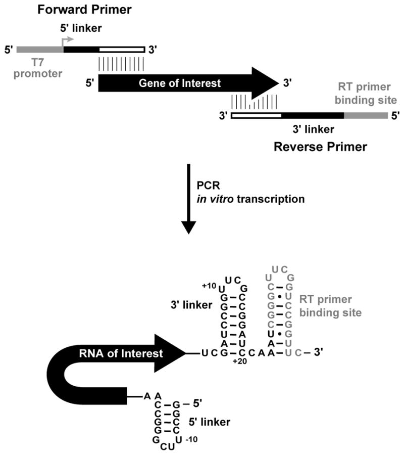
Structure cassette design for in vitro RNA synthesis. (Adapted from Fig. 7 in Merino et al., 2005).

4.2. DURATION

Preparation	1 hour
Protocol	2 days

See Figure 5.1 for a flowchart overview of the protocol.

Figure 5.1.

Flowchart overview of the entire strategy for modeling RNA secondary structure, based on SHAPE experimental information.

5. STEP 1 RNA FOLDING AND SHAPE TREATMENT

5.1 Overview

Fold the RNA in a SHAPE-compatible buffer (here we use a HEPES buffer, a Tris-EDTA buffer may also be used) in the presence of ligand (if required) and add SHAPE reagent.

5.2 Duration

1.5–2.5 hours

• 1.1Add 2 μL of 5 μM RNA (10 pmol) to 10 μL of RNase-free water to a 0.65 mL microcentrifuge tube.
• 1.2Heat mixture at 95 °C for 2 min then immediately place on ice for 2 min.
• 1.3Add 6 μL of 3.3× folding buffer and mix well.
• 1.4Incubate at 37 °C for 20 min to allow RNA to refold.
• 1.5To a fresh 0.65 mL tube, add 2 μL of water or ligand (for example, 50 mM TPP) (see Tip 5.4).
• 1.6Add 18 μL of folded RNA from step 1.4 to this tube and mix well.
• 1.7Incubate at 37 °C for 10 min to allow ligand binding.
• 1.8Make a fresh stock of 80 mM SHAPE reagent (1M7, 1M6, or NMIA).
• 1.9To a 0.65 mL tube add 1 μL of 80 mM SHAPE reagent; label (+). To another 0.65 mL tube add 1 μL of neat DMSO; label (−).
• 1.10Add 9 μL of folded RNA to the (+) tube. Mix quickly by pipetting and incubate at 37 °C. Incubate 3 min for 1M6 or 1M7 reagents or 22 min for NMIA (see Tip 5.5).
• 1.11Add 9 μL of folded RNA to the (−) tube for the no reagent control. Mix quickly and incubate for the same amount of time as the (+) sample.
• 1.12Perform an ethanol precipitation. To each reaction add 90 μL RNase-free water, 4 μL 5 M NaCl, 1 μL glycogen (20 mg/mL), 240 μL ethanol. Mix well. Incubate at −80 °C for 30 min followed by centrifugation in a microfuge at 4 °C for 30 min at maximum speed.

5.3. Tip

Following the modification, the 1M7 treated sample will change color from yellow to orange. 1M6 and NMIA reactions do not change color.

5.4. Tip

If studying ligand effects on RNA structure, perform the steps in section 5.2 multiple times in parallel, varying the ligand concentration in step 1.5.

5.5. Tip

The SHAPE reagent incubation time is dependent on temperature and pH of the system studied. Incubation times will be longer at lower temperatures and more acidic pH. At 5 half-lives the SHAPE reagent will be mostly consumed by the competing hydrolysis reaction. Depending on buffer conditions and temperature, incubation time may need to be optimized. Reagent kinetics can be readily determined by monitoring formation of the hydrolysis product (Merino et. al, 2005; Mortimer & Weeks, 2007).

6. STEP 2 PRIMER EXTENSION

6.1 Overview

Perform reverse transcription to detect sites of SHAPE modification, and sequencing to enable electropherogram peak alignment.

6.2 Duration

2 hours

• 1.1Prepare 411 Master Mix.
• 1.2In two 0.65 μL tubes from the last step in section 5, resuspend the pelleted RNA (about 2.5 pmol each) from the (+) and (−) SHAPE samples in 11 μL water or 10 μL water and 1 μL Superase-In RNase inhibitor (optional).
• 1.3In a new 0.65 μL tube, combine 5 pmol RNA and water to 10 μL; label “Sequencing”.
• 1.4To each of the (+), (−), and sequencing tubes, add 2 μL fluorescently labeled reverse transcription primer, 1.25 μM, (2.5 pmol) and mix by pipetting (see Tips 6.3 and 6.4).
• 1.5Incubate 5 min at 65 °C.
• 1.6Incubate 3 min at 45 °C.
• 1.7Place on ice 2 min.
• 1.8Add 6 μL 411 Master Mix to each of the (+) reagent, (−) reagent, and sequencing tubes.
• 1.9 Add

  1 μL SuperScript III to each tube and mix well.

• 1.10Sequencing tube only: Add 1 μL ddC, ddA, or ddT, 10 mM, or 1 μL ddG, 0.25 mM. (concentration of dideoxynucleotide may need to be adjusted empirically, see Tip 7.5).
• 1.11Incubate 1 min at 45 °C.
• 1.12Incubate 40 min at 52 °C.
• 1.13Incubate 10 min at 65 °C, then hold at 4 °C.
• 1.14Optional: Add 1 μL glycogen to sequencing tube only, 20 mg/mL (may facilitate recovery of small nucleic acids).
• 1.15Add 120 μL absolute ethanol to each tube and mix well. Incubate at −80 °C for 30 min (see Tip 6.5).
• 1.16Centrifuge 30 min at >10,000 g (at 4 °C if possible).
• 1.17Carefully discard supernatant.

  • Optional steps to reduce salt carry-over (recommended):

    • 1.17aRinse pellet with 500 μL 80% ethanol, do not disturb the pellet.
    • 1.17bCentrifuge 5 min at >10,000 g.
    • 1.17cDiscard supernatant.

  • Repeat steps 1.17a-c twice.

• 1.18Let pellets dry 5 min at room temperature.
• 1.19Resuspend each pellet in 10 μL hi-di formamide.
• 1.20Denature at 95 °C for 2 min.

6.3. Tip

Select fluorophores that are supported by the specific capillary electrophoresis instrument to be used, and consider which pairs of samples will ultimately be analyzed in the same capillary. For example, in the widely supported G5 dye set, use the fluorophore VIC to produce (+) or (−) SHAPE cDNA and the fluorophore NED for sequencing. 5-FAM and 6-JOE are also commonly used as a compatible dye pair. QuShape supports mobility shift correction for the following fluorescein-derived dyes: 5-FAM, 6-FAM, TET, HEX, 6-JOE, NED, and VIC.

6.4 Tip

Two sequencing reactions can be used for RNAs that are difficult to align SHAPE reactivities to a reference sequence. Use a different fluorophore for each type of dideoxynucleotide being used so that both sequencing reactions will be able to be analyzed in the same capillary.

6.5. Tip

The salt remaining from the primer extension reaction is sufficient for the ethanol precipitation. No extra NaCl is required.

6.6. Tip

For the ethanol precipitation of the (+) and (−) SHAPE reactions following primer extension, additional glycogen is not needed since it will carry through from the first precipitation (step 1.14).

7. STEP 2 CAPILLARY ELECTROPHORESIS

7.1 Overview

Resolve products of primer extension reactions by capillary gel electrophoresis.

7.2 Duration

1.5 hours

• 2.1For each sample, load ~1.5 pmol cDNA and ~0.5 pmol sequencing cDNA in 8–12 μL hi-di formamide in a single plate well. These concentrations may require adjustment for different CE instruments (see tips below).
• 2.2 Electrophorese

  samples according to instrument protocol. This step is typically automated.

7.3. Tip

The dynamic range of CE fluorescence detectors is typically rather small, and over-saturation of the signal can easily occur. This artifact manifests as high, flat, “clipped” peaks in the electropherogram. Some clipping on the 5′ and 3′ ends of the trace is normal and tolerable, but clipping in the center of the trace is undesirable. If this occurs, fill the capillaries with new polymer to flush out any residual cDNA molecules, load a lower concentration of cDNA in each well, and re-run. DO NOT use over-saturated electropherograms for SHAPE analysis or structure modeling.

7.4. Tip

Sequencing reactions may be performed on a larger scale (20–50×) and the products stored for re-analysis by freezing in formamide at 4 °C or −20°C in the dark.

7.5. Tip

Sequencing reactions are very sensitive to the ratio of ddNTP terminator to dNTPs and may not be successful without optimization. Run 0.5 pmol of the sequencing products alone on the CE instrument to ensure success before mixing with experimental samples.

8. STEP 3 DATA PROCESSING USING QUSHAPE

8.1. Overview

The QuShape analytical computer program performs a series of data processing operations to calculate SHAPE reactivities based on the CE-generated data that has been recorded in ABIF files (see http://www.chem.unc.edu/rna/qushape/). The user controls QuShape via a graphic interface. This interface includes the main Data View window, the Tool Inspector window, and the Script Inspector window (Fig. 8.1). Results of every operation are plotted in the Data View window, allowing the user to monitor the quality of each data processing step. As a default, selection of each successive data processing step is automatic. The standard procedure is for the user to execute each tool as it appears in the Tool Inspector window (by clicking the Apply button), inspect the result in the Data View window, and proceed to the next tool in the default sequence (by clicking the Done button). However, if the user is not satisfied with the results of the automatic procedure, the Tool Inspector window offers the user additional analytical tools and parameter controls that can be employed by clicking on them.

Figure 8.1.

QuShape graphical user interface. The main Data View window (center) displays the results of the most recently performed operation. The Tool Inspector window (upper right) displays user-controlable parameters and options for the selected tool, which allow manual control over each algorithmic step in instances where the default execution is not satisfactory. The Script Inspector window (lower right) lists the sequence of tools applied thus far to the data. (A) Screenshot of the QuShape display at the completion of the Sequence Alignment step. The main window displays four electropherograms traces: (+) SHAPE reaction signal (RX); (−) SHAPE reaction signal (BG); ddNTP sequencing signal in the (+) reaction capillary (RXS1); and ddNTP sequencing signal in the (−) reaction capillary (BGS1). The matched peaks in the four traces are indicated by vertical lines. Peaks classified as specific are labeled G at the bottom of the window, while peaks classified as non-specific are labeled N. The optimally aligned RNA nucleotide sequence is also displayed at the bottom of the window. (B) Screenshot of the QuShape display at the completion of the Reactivity step. The main window displays the normalized reactivities of the nucleotides.

8.2. Duration

5–20 min depending on RNA length

See Figure 8.2 for a flowchart overview of the protocol.

• 1.1Create a new project by clicking New Project in the File menu. Enter the name of the project and select the directory that contains the raw CE data files. Select the project type. If there is just one sequencing lane in each capillary in the files obtained from electrophoresis, select One Sequencing Channel. Otherwise select the second option, Two Sequencing Channels. Press the Next button to go to next step.
• 1.2Select CE data files using the Browse button. Text- or ABIF-formatted (+) Reaction and (−) Reaction files are both acceptable. The RNA Sequence file (.txt, .seq, .fasta) or a Reference Project (Ref. Proj.) file (.qushape) are selected in the same way. Click the Next button to go to the last step of creating a new project.
• 1.3Select the channel numbers. Select channels in the (+) Reaction Channels panel to specify RX and RXS1 (RX and RXS refer to the SHAPE reaction signal and the sequencing signal, respectively, in the presence of reagent). For the sequencing ladder, the ddNTP type (ddC, ddG, ddT, ddA) must be selected. Repeat the same for BG and BGS1 in the (−) Reaction Channels panel (BG and BGS refer to the SHAPE reaction signal and the sequencing signal, respectively, in the absence of reagent). If there is another sequencing lane, RXS2 and BGS2 should be selected in the (+) and (−) Reaction Channels panels, respectively. After specifying all the channels, press the Apply button to view the data display in the Data View window. If all selections are correct, press the Done button to proceed to the analysis. If there is a problem with specified options, use the Back button to go to the previous dialog to change the parameters.
• 1.4Select the region of interest (ROI) along the elution time axis using the Region of Interest tool: Either type the elution time values of the start and end points directly in the boxes in the Tool Inspector window or, more conveniently, select the start point of the ROI by pressing and holding down the ‘F’ (from) key on the keyboard and then placing the mouse arrow at the desired elution time position in the plot in the Data View window and clicking the left mouse button. The end point of the ROI is selected similarly by pressing and holding down the ‘T’ (to) key, and then placing the mouse arrow at the desired elution time position in the Data View window and clicking the left mouse button. Once the start and end points of the ROI are entered, the user-chosen ROI will be displayed in the Data View window on a gray background.
• 1.5Apply the Smoothing tool to filter out high-frequency noise in the data and correct saturated data points. If not satisfied with the default results, the user can select a different smoothing method and/or change the width of the smoothing filter in the Window Size box. Unchecking Saturation Correction option disables correction of saturated points in the trace.
• 1.6Apply the Mobility Shift tool to align pairs of signals within each capillary. Use the selection boxes to change dye type of each trace if the automatically shown dye type, determined during the project creation step, is incorrect.
• 1.7Apply the Baseline Adjustment tool to remove baseline offset by specifying the baseline window. Baseline is defined by the minima of a set of consecutive elution time intervals whose length is specified in the Baseline Window (default value is 60). If smoothing of the baseline drift is desired, the Smooth the Baseline Drift box should be checked.
• 1.8Apply the Signal Decay Correction tool. Automatic Summation is the default method to correct gradual signal decay. If not satisfied, select either Exponential method or Summation method. The Summation method is the same method as the automatic approach, but the user to determine the value of the key parameter, Factor.
• 1.9Apply the Signal Alignment tool to align pairs of signals across two capillaries. After this alignment procedure is finished, the aligned RX and BG signals will be plotted superimposed in one panel in the Data View window and the aligned RXS and BGS signals will be plotted superimposed in the other panel, so that the accuracy of the alignment can be checked visually. If misalignment is found, it can be corrected manually after clicking the Modify Matched Peaks button.
• 1.10Apply the Sequence Alignment tool to assign each peak in the (+) SHAPE reaction and (−) SHAPE reaction signals to their corresponding RNA position. Once this operation is finished, the display in the Data View window will change to a view in which corresponding peaks in RX, BG, and BGS traces are linked by vertical arrows (Fig. 8.1A). The results of base-calling and sequence alignment will be shown at the bottom of the BGS panel; the top row shows the RNA sequence and the bottom row shows the results of base calling. If the alignment is not accurate, the errors can be corrected manually.
• 1.11Apply the Reactivity tool to calculate SHAPE reactivities for all nucleotides in the selected region of interest based on their peaks in the (+) SHAPE reaction and (−) SHAPE reaction signals. This tool performs three operations. First, a whole-signal Gaussian integration is performed for all peaks in the (+) and (−) reaction signals, fitting each peak with a Gaussian function individually optimized for position, height, and width. Next, the scaling operation scales the BG signal relative to the RX signal. This scaling is necessary because the (+) and (−) reaction primer extension reactions were performed separately and not necessarily under fully identical conditions. When the Reactivity tool is open, the scaling factor is computed automatically and is displayed in the Scale Factor window (Fig. 8.1B). When the Reactivity tool is executed, by clicking the Apply button, the BG signal will be scaled by this factor. If not satisfied, other scaling factor values can be tested by entering them in the Scale Factor window. Finally, the normalization operation subtracts the integrated values for the (−) reaction peaks from the (+) reaction peaks, and normalizes the difference to obtain the normalized nucleotide-resolution reactivity for every RNA position.

  A box normalization-based algorithm is used to normalize data. This normalization scales reactivities to a scale spanning 0 to ~2, where zero indicates no reactivity and 1.0 is the average intensity for highly reactive RNA positions. Nucleotides with normalized SHAPE reactivities 0–0.40, 0.40–0.85, and >0.85 correspond qualitatively to unreactive, moderately reactive, and highly reactive positions, respectively, and are plotted in different colors. As a part of the normalization procedure, the percent of outliers is determined automatically and is displayed in the Outlier window. A different percentage can be selected. There are three alternative displays of the output of the Reactivity tool: (1) “Reactivity” button plots the normalized reactivities of all nucleotides; (2) “Peak Area” button plots the areas of RX and BG peaks; (3) “Data” button draws the same plot as provided through the Sequence Alignment tool (linked RX, BG, RXS, and BGS traces, as well as the nucleotide sequence); in addition, it overlays each peak in RX and BG traces with its Gaussian estimation.

• 1.12Apply the View Report tool to output the computed nucleotide SHAPE reactivities. The final report of QuShape data processing is displayed as a table in the Tool Inspector window. This table contains the following information about each nucleotide: SeqNum – nucleotide number; seqRNA – nucleotide base type; posSeq – position of the nucleotide in the sequence ladder; posRX – position of the RX peak; areaRX – area of the RX peak; posBG – position of the BG peak; areaBG – area of the BG peak; areaDiff – difference between RX and BG areas; normDiff – normalized difference (the normalized reactivity of the nucleotide). This table can be saved as a tab-delimited text file by clicking the ‘Save as Text’ button.

Tip 8.3

QuShape runs under Windows, MacOS/X, and Linux, and uses open-source software. Its downloading and installation instructions can be found in the Installation Guide section at http://www.chem.unc.edu/rna/qushape/.

Tip 8.4

Some of the tools are computationally intensive, and their execution can take tens of seconds. During their execution (after pressing the Apply button), the left-bottom corner of the screen will display the “Applying…” message. Once the operation is finished, this message will change to “Applied”, and the Done button in the Tool Inspector window will become enabled (its appearance will change from dim to sharp contrast).

Tip 8.5

The start and the end segments of electropherogram traces typically have stretches of excessive and undifferentiated fluorescence that obscure peaks corresponding to the nucleotides at the either end of the studied RNA. The region of interest (ROI) must be selected, using the Region of Interest tool, along the elution time axis to avoid these unusable segments.

Tip 8.6

After the signal alignment procedure is finished, the accuracy of the alignment can be checked visually. If misalignment is found, it can be corrected manually after clicking the Modify Matched Peaks button. This will change the display: RXS signal will be plotted above BGS signal and vertical lines will be drawn linking a subset of the matched peaks in the two signals. An incorrect link between two peaks in the two signals can be changed by pressing and holding the ‘Shift’ key while placing the mouse arrow on the wrong peak, clicking and holding the left mouse button, and dragging the link to the desired peak. If a new link is desired, press and hold the ‘A’ key while clicking with the mouse on the two peaks that should be linked. If a link must be removed, press and hold the ‘D’ key while clicking on that link with the mouse. Once all the desired link changes are made, click the Apply button to realign the two signals according to the newly imposed constraints.

Tip 8.7

In the sequence alignment step, the Base Calling box should be used if the user wants to come back to the sequence alignment after pressing the ‘Done’ button and moving to other tools. In that case, the Sequence Alignment tool can be called from the Sequence menu with the base-calling operation enabled, so that upon execution of this tool the previous manually corrected base assignments will be discarded. Therefore, the Base Calling box should be unchecked if you want to use previously obtained base-calling results.

Tip 8.8

If the sequence alignment is not accurate, the errors can be corrected manually. Four different manual correction operations are available:

1. The base label of a peak in the BGS trace can be changed. For example, suppose that ddC was used for sequencing. Consequently, the bottom row consists of ‘N’ and ‘G’ labels. Clicking on ‘N’ with the mouse will turn it to ‘G’. Clicking on ‘G’ will turn it to ‘N’.

2. An extra base can be added to the bottom row. By pressing and holding the ‘A’ key while clicking at a particular location in the bottom row with the mouse, an ‘N’ will be inserted at that location and this added nucleotide will be linked to RX and BG.

3. A base and corresponding links can be deleted by pressing and holding the ‘D’ key while clicking at a base.

4. Computed locations of the peak centers in BG and RX can be moved by pressing the ‘Shift’ key and dragging the arrow to the desired location.

After modifying the sequences, press Apply to see the new alignment with nucleotides matched to the peaks in RX and BG. Note that at this time the base calling operation will be disabled. If this operation needs to be performed again, check the Base Calling box.

Tip 8.9

In the reactivity step, the scaling factor is automatically determined for the entire BG data set, and all BG signals are scaled by this factor. When working with very long sequences, it may be more accurate to scale BG locally, rather than globally. To use local scaling, check the ‘Scale by Windowing’ box (Fig. 8.1B).

9. STEP 4 DATA PROCESSING AND RNA MODELING

9.1 Overview

Prepare files needed for RNA secondary structure modeling, then use the software package RNAstructure (Reuter & Mathews, 2010) to generate models. All python scripts indicated below are freely available from the Weeks lab website (http://www.chem.unc.edu/rna/qushape.

9.2 Duration

20 min hands-on time

0–6 h computer time (depending on sequence length)

• 1.1Using a spreadsheet editor or text editor, format the report file obtained at the end of QuShape data processing into two columns consisting of nucleotide number and SHAPE reactivity value. Positions where data quality is poor, such as those with high background in the DMSO control, or where SHAPE reactivity could not be determined should be entered as “−999”. Save this file as a “.txt” file or “windows formatted text” from Excel. Numbering should start at 1 and the file should contain as many nucleotides as the RNA being modeled. Each experiment (e.g., 1M7, 1M6, NMIA) should have its own file.
• 1.2Use the python script “simple2boxplot.py” to normalize the 1M7 SHAPE reactivities with the boxplot method. With the normalization script in the same folder, type: “python simple2boxplot.py fileIN.txt fileOUT.txt”, where “fileIN” is the formatted 1M7 file from the previous step. Change “fileOUT” to a unique name for the outputted file. The output of this script will be boxplot normalized 1M7 SHAPE reactivities suitable for folding.
• 1.3Use the python script “boxplot2simple.py” to normalize the 1M6 SHAPE reactivities using the “simple” normalization method. With the normalization script in the same folder, type: “python boxplot2simple.py fileIN.txt fileOUT1M6.txt”, where “fileIN” is the formatted 1M6 file from step 1.1. Change “fileOUT1M6.txt” to a memorable and unique name that will contain the outputted simple normalized 1M6 reactivities.
• 1.4Repeat step 1.3 for the NMIA SHAPE reactivities.
• 1.5Use the python script “differenceByWindow.py” to subtract the normalized 1M6 SHAPE reactivities from the NMIA reactivities.
  • 1.5aAt the command prompt type “python differenceByWindow.py nmia.txt 1m6.txt differenceOUT.txt 25”. The input files for the difference calculating script (nmia.txt and 1m6.txt) are the resulting files from steps 1.4 and 1.3, respectively. The last argument of the command, “25”, defines the window size for the sliding baseline.
  • 1.5bWhen the command is finished running, a graph will appear showing the result of the difference calculation before and after using a sliding window difference. The differential SHAPE reactivities should occur sparsely throughout the length of the RNA and be roughly evenly distributed across positive and negative amplitudes (Fig. 9.1, bottom). In rare cases, alternative window sizes may need to be tried until suitable parameters are found.
• 1.6Using a web browser, go the RNAstructure online structure prediction server at: http://rna.urmc.rochester.edu/RNAstructureWeb/Servers/Predict1/Predict1.html
• 1.7Fill out the fields on the web form. Make sure to include a sequence title, the RNA sequence, and an email address.
• 1.8Under the optional data heading, choose to upload a SHAPE constraints file. Select the boxplot normalized 1M7 file (step 1.2).
• 1.9Also under the optional data heading, choose to upload the calculated difference file. Select the file from step 1.5.
• 1.10Enjoy a cup of coffee while your RNA folds. You will receive an email when the secondary structure modeling is complete. The effect of including differential SHAPE reactivity information is illustrated in Fig. 9.2.

Figure 9.1.

Differential SHAPE analysis of the E. coli 5S rRNA. Normalized SHAPE reactivities from reactions with NMIA (top) and 1M6 (middle) are highlighted by nucleotide reactivity. Differential SHAPE reactivities (bottom) were calculated by first scaling 1M6 to NMIA reactivities over a moving window and then subtracting 1M6 from NMIA reactivities. Strong differential reactivity enhancements (>|0.3| SHAPE-units) are colored gray. Nucleotide positions showing strong positive-amplitude (favoring NMIA) differential reactivities are labeled. (Adapted from Fig. 2 (in color) in Rice et al., 2014).

Figure 9.2.

Representative secondary structure modeling for the 5S rRNA without and with SHAPE data. Base pair predictions are illustrated with lines (black, dashed gray, and solid gray denoting correct, incorrect, and missing base pairs, respectively) on conventional secondary structure representations (top) and circle plots (bottom). Nucleotides are highlighted according to their SHAPE reactivity on a black, gray, white-filled scale for low, medium, and strong reactivity. Nucleotides showing strong preferential reactivity with NMIA (>0.3 units) are indicated with a delta symbol. (Adapted from Fig. 3 (in color) in Rice et al., 2014).

Tip 9.3

Step 1.5, the script “differenceByWindow.py” will crash if there is a stretch of no data larger than the window size given. It may be necessary to perform this step in two parts (where there is data present) and then recombine the separate files.

Tip 9.4

For step 1.5b, windows sizes between 15 and 50 are reasonable. Selection of lower numbers results in more aggressive reactivity matching. This parameter can usually be left at 25. The real window size is calculated as 2n+1. Setting this parameter to 25 thus results in a 51 nucleotide centered sliding window.

Tip 9.5

For step 1.5b, a slight bias toward positive amplitude differential SHAPE signals is fine.

See Figure 9.3 for the flowchart for the complete protocol.

Figure 9.3.

Flowchart for RNA secondary structure modeling using the full three-reagent SHAPE experiment, analyzed using RNAstructure.

Figure 8.2.

Flowchart for automated processing of SHAPE data, quantified by capillary electrophoresis, using QuShape.