

Abstract
The contrast sensitivity function (CSF) has shown promise as a functional vision endpoint for monitoring the changes in functional vision that accompany eye disease or its treatment. However, detecting CSF changes with precision and efficiency at both the individual and group levels is very challenging. By exploiting the Bayesian foundation of the quick CSF method (Lesmes, Lu, Baek, & Albright, 2010), we developed and evaluated metrics for detecting CSF changes at both the individual and group levels. A 10-letter identification task was used to assess the systematic changes in the CSF measured in three luminance conditions in 112 naïve normal observers. The data from the large sample allowed us to estimate the test–retest reliability of the quick CSF procedure and evaluate its performance in detecting CSF changes at both the individual and group levels. The test–retest reliability reached 0.974 with 50 trials. In 50 trials, the quick CSF method can detect a medium 0.30 log unit area under log CSF change with 94.0% accuracy at the individual observer level. At the group level, a power analysis based on the empirical distribution of CSF changes from the large sample showed that a very small area under log CSF change (0.025 log unit) could be detected by the quick CSF method with 112 observers and 50 trials. These results make it plausible to apply the method to monitor the progression of visual diseases or treatment effects on individual patients and greatly reduce the time, sample size, and costs in clinical trials at the group level.
Keywords: contrast sensitivity function, specificity, sensitivity, accuracy, Bayesian
Introduction
In clinical vision science, the lack of precise tests for evaluating functional vision change has been a major limiting factor in the diagnosis and treatment of eye disease. Current shortcomings in functional vision tests include unsatisfactory precision, poor test–retest reliability, and insensitivity to visual changes caused by conditions or diseases. Visual acuity (VA), the most common functional test in clinical vision, may not be ideal for characterizing visual deficits (Hess & Howell, 1977; Jindra & Zemon, 1989; Marmor, 1981, 1986; Marmor & Gawande, 1988; Montes-Mico & Ferrer-Blasco, 2001; O'Donoghue, Rudnicka, McClelland, Logan, & Saunders, 2012; Onal, Yenice, Cakir, & Temel, 2008; Yenice et al., 2007) and is insensitive to early stages of eye diseases and progressive declines in functional vision (Marmor, 1986; Owsley, 2003; Yenice et al., 2007). Onal et al. (2008) reported that patients with early glaucoma had good VA but showed reduced contrast sensitivity at all spatial frequencies. O'Donoghue et al. (2012) found that the sensitivity in detecting hyperopia based on uncorrected VA was only 44%. The Humphrey visual field test, another widely used tool in clinical vision, also exhibits poor test–retest reliability. It has been reported that 85.9% of the initial abnormal visual fields assessed in the Ocular Hypertension Treatment Study were not verified on retest (Keltner et al., 2000).
As a fundamental assay of spatial vision that describes performance over a wide range of spatial frequencies, the contrast sensitivity function (CSF) exhibits promise as a functional vision endpoint (Ginsburg, 2003). The CSF is closely related to daily functional vision, which can be used to characterize visual performance in both normal and impaired vision (Arden & Jacobson, 1978; Ginsburg, 1981, 2003; Hess, 1981; Hess & Howell, 1977; Jindra & Zemon, 1989; Onal et al., 2008; Richman et al., 2010; Shandiz et al., 2010). It has also shown promise for monitoring the progression of vision loss in eye diseases or their remediation with treatment (Barnes, Gee, Taylor, Briggs, & Harding, 2004).
Despite its clinical promise, the precise and efficient assessment of the CSF is challenging. The conventional CSF tests can be either fast or precise, but not both. The various CSF charts are fast and convenient to use, but the sparse sampling of both spatial frequency and stimulus contrast renders the tests rather imprecise (Bradley, Hook, & Haeseker, 1991; Buhren, Terzi, Bach, Wesemann, & Kohnen, 2006; Hohberger, Laemmer, Adler, Juenemann, & Horn, 2007; Pesudovs, Hazel, Doran, & Elliott, 2004; van Gaalen, Jansonius, Koopmans, Terwee, & Kooijman, 2009). The laboratory CSF tests can be precise but may require 500 to 1,000 trials and take about 30 to 60 min (Harvey, 1997; Kelly & Savoie, 1973). Such testing times might be acceptable for measuring a single CSF in the laboratory but are prohibitive in situations requiring assessment of CSF in clinical settings, especially when multiple CSFs need to be assessed (e.g., for the left and right eyes).
In an attempt to achieve both high precision and efficiency in CSF assessment, Lesmes et al. (2010) developed the quick CSF method, which applies a Bayesian adaptive algorithm to estimate the full shape of the CSF and tests observers with the optimal stimulus that is selected in the two-dimensional contrast and spatial frequency space (see Figure A1 in Appendix A) to maximize the expected information gain in each trial. They showed that CSFs measured with the quick CSF method were precise and exhibited excellent agreement with CSFs obtained independently using a conventional method. Recently, the efficiency of the quick CSF method was further improved another 2.5 times by incorporating a 10-alternative forced-choice letter identification task (Hou, Lesmes, Bex, Dorr, & Lu, 2015).
The CSFs obtained with the quick CSF method have also been shown to be precise and accurate in many other experimental conditions, including peripheral vision (Rosén, Lundström, Venkataraman, Winter, & Unsbo, 2014) and in second-order perception (Reynaud, Tang, Zhou, & Hess, 2014), and in clinical populations, such as patients with amblyopia (Hou et al., 2010), age-related macular degeneration (AMD) (Lesmes, Wallis, Jackson, & Bex, 2013; Lesmes, Wallis, Lu, Jackson, & Bex, 2012), glaucoma (Ramulu, Dave, & Friedman, 2015), and normal age-related visual changes (Jia, Yan, Hou, Lu, & Huang, 2014). The quick CSF method has been utilized in various empirical studies to investigate the dynamic effects of visual adaptation (Gepshtein, Lesmes, & Albright, 2013) and the effects of emotional arousal on CSF (Lee, Baek, Lu, & Mather, 2014). With the help of the quick CSF method, Kalia et al. (2014) found surprising visual development in a unique sample of patients who experienced extended early-onset blindness before removal of bilateral cataracts.
Although it has demonstrated great potential as a clinical tool, the quick CSF method has been tested with relatively small samples or under a single experimental condition (Dorr, Lesmes, Lu, & Bex, 2013; Hou et al., 2010; Lesmes et al., 2010). Its precision and test–retest reliability have yet to undergo more rigorous tests. Furthermore, the performance of the quick CSF method in detecting CSF changes between different conditions has not been extensively studied. A large sample study is necessary for us to fully evaluate the performance of the quick CSF procedure in terms of its precision, test–retest reliability, and performance in detecting CSF changes at both the individual and group levels.
A full evaluation of the precision of the quick CSF method requires a large sample study on naïve observers. The quick CSF method assumes that all observers have the same slope in their psychometric function; its performance depends on the actual slope of the psychometric function of individual observers (Hou et al., 2010, 2015). A large sample study would allow us to evaluate the distributional properties of the precision metric and provide a much more rigorous examination of the method. In addition, we need a new procedure for evaluating the test–retest reliability of the quick CSF method. Previously, we assessed the test–retest reliability of the quick CSF method with the correlation between repeated measures of contrast sensitivity across all spatial frequencies for each observer (Hou et al., 2015; Lesmes et al., 2010). The assessment is inadequate because, due to the underlying assumption of the log parabola CSF model, the contrast sensitivities measured by the quick CSF method are highly constrained. A large sample study would allow us to develop a new procedure for assessing the test–retest reliability of the quick CSF method by computing the correlation of contrast sensitivity with independent groups of subjects in different spatial frequency conditions.
Another purpose of the study is to develop methods for detecting CSF changes at both the individual and group levels and evaluating the performance of the quick CSF method in detecting CSF changes. At the individual level, the ability to detect CSF changes provides important bases for diagnosing the progression of vision loss in eye disease or the treatment response. At the group level, the ability to detect CSF changes can provide decisive evidence to judge the safety and efficacy of treatments. The Bayesian parametric nature of the quick CSF method makes the measurement very information-rich. It provides not only a (conventional) point estimate but also the posterior distribution of the estimate of interest that can be exploited to test and detect CSF changes of an individual in different conditions. At the group level, posterior distributions of the estimate of interest from multiple observers can be combined to test and detect CSF changes. We develop and test these methods in the current study.
To evaluate the performance of the quick CSF method in detecting CSF changes, we manipulated luminance conditions in the study to create CSF changes to mimic the effect sizes of CSF changes that are commonly observed in clinical settings. For example, patients with open angle glaucoma exhibited no impairment in VA but a 0.15 log10 unit decrease in Pelli-Robson contrast sensitivity (Haymes et al., 2006). Similarly, patients in the early stage of AMD with normal or near-normal VA exhibited a 0.15 log unit (Kleiner, Enger, Alexander, & Fine, 1988) or a 0.34 log unit (Midena, Degli Angeli, Blarzino, Valenti, & Segato, 1997) area under the log CSF (AULCSF) decrease depending on the severity of their disease. Patients with AMD and characteristic macular changes or neovascular AMD exhibited a 0.45 log unit Pelli-Robson contrast sensitivity reduction (Bellmann, Unnebrink, Rubin, Miller, & Holz, 2003). Kalia et al. (2014) found that the average improvement in AULCSF is 0.53 log unit for the five patients who gained significant vision improvement after cataract surgery. Owsley, Sekuler, and Siemsen (1983) found that the AULCSF decreased by 0.31, 0.48, and 0.57 log unit for people in their 60s, 70s, and 80s, respectively. These results in the literature suggest that 0.15, 0.30, and 0.45 log unit AULCSF changes correspond to mild, medium, and large CSF changes in clinical populations. We therefore carefully chose three different luminance conditions (2.62, 20.4, and 95.4 cd/m2) to create similar AULCSF changes in this study (0.14, 0.29, and 0.43 log unit; see Results). Similar settings were also used in other studies (Dorr et al., 2013; Kooijman, Stellingwerf, van Schoot, Cornelissen, & van der Wildt, 1994).
In this study, we recruited 112 college students and applied the quick CSF method to assess CSF in three luminance conditions, evaluated the distribution of the precision of CSF measures, developed methods for assessing the test–retest reliability of the quick CSF method to test and detect CSF changes, and evaluated the performance of the quick CSF method in detecting CSF changes at both the individual and group levels. The large sample size was necessary to further assess the precision, the test–retest reliability of the quick CSF method, and its performance in detecting CSF changes with minimal assumptions. Empirical power analyses for detecting CSF changes based on the group data were also conducted. We show that the quick CSF method is reliable and sensitive in detecting commonly observed CSF changes at both the individual and group levels.
Method
Observers
A total of 112 college students from The Ohio State University participated in the study to obtain partial course credit in an introductory psychology course. All observers had normal or corrected-to-normal vision and were naïve psychophysical observers. Verbal consent was obtained before the experiment. The study protocol was approved by the institutional review board of human subjects research of The Ohio State University and adhered to the tenets of the Declaration of Helsinki.
Apparatus
All programs were written in Matlab (The Mathworks Corp., Natick, MA) with Psychtoolbox subroutines (Kleiner, Brainard, & Pelli, 2007) and run on a personal computer. Stimuli were displayed on a gamma-corrected Samsung (Seoul, South Korea) UN55FH6030 55-in. LED monitor with a mean luminance of 95.4 cd/m2. The resolution was 1920 × 1080 pixels, and the vertical refresh rate was 60 Hz. A bit-stealing algorithm was used to achieve 9-bit grayscale resolution (Tyler, 1997). Participants viewed the display binocularly from a distance of 4 m in a dark room.
Four viewing conditions were tested in the experiment: low luminance (L), medium luminance (M), high luminance (H), and low pass (LP). In the H condition, subjects viewed the display through uncovered goggles. In the M condition, subjects viewed the display binocularly through goggles with neutral density filters with an attenuation factor of 0.67 decimal log unit. In the L condition, subjects viewed the display through goggles fit with two neutral density filters with a total optical density of 1.56 log units. Bangerter occlusion foils were used as the low pass filter in the LP condition. The data in the LP condition are analyzed separately and are not presented in this article. The equivalent mean luminance in the L, M, and H conditions was 2.62, 20.4, and 95.4 cd/m2, respectively. Compared with the L condition, there were 7.8 and 36.4 folds of luminance change in the M and H conditions, respectively. The magnitudes of luminance change were comparable with those used in previous studies (Dorr et al., 2013; Kooijman et al., 1994).
Stimuli
Ten filtered Sloan letters—C, D, H, K, N, O, R, S, V, and Z—were used as stimuli (Alexander, Xie, & Derlacki, 1994; Hou, Lu, & Huang, 2014; Figure 1a). The letter images were filtered with a raised cosine filter (Chung, Legge, & Tjan, 2002):
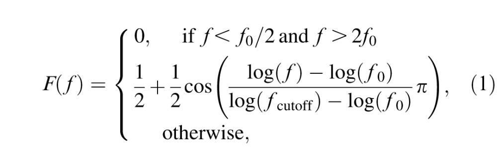 |
where f denotes the radial spatial frequency, f0 = 3 cycles per object is the center frequency of the filter, and fcutoff = 2f0 was chosen such that the full bandwidth at half height is one octave. The pixel intensity of each filtered image was normalized by the maximum absolute intensity of the image. After normalization, the maximum absolute Michelson contrast of the image is 1.0. Stimuli with different contrasts were obtained by scaling the intensities of the normalized images with corresponding contrast values. Stimuli with different spatial frequencies were generated by resizing (Figure 1b). There were 128 possible contrasts (evenly distributed in log space from 0.002 to 1) and 19 possible spatial frequencies (evenly distributed in log space from 1.19 to 30.95 cycles per degree [cpd]). The narrow band filtered letters can provide assessment of contrast sensitivity in different central spatial frequencies that are equivalent to that with sinewave gratings (Alexander et al., 1994; McAnany & Alexander, 2006).
Figure 1.

(a) Ten filtered Sloan letters. (b) Filtered letter C in several spatial frequency conditions. (c) Triletter stimuli.
Implementation of the quick CSF method
In the quick CSF method, CSFs are characterized by a truncated log parabola with four parameters (see Figure A1 in Appendix A): peak gain gmax, peak spatial frequency fmax, bandwidth at half height β (in octaves), and low frequency truncation level δ (Lesmes et al., 2010; Watson & Ahumada, 2005). In the rest of the article, we use CSF parameters interchangeably with truncated log parabola parameters unless otherwise stated. Unlike many conventional methods that select stimuli adaptively only in the contrast space, the quick CSF method selects optimal stimuli in the two-dimensional contrast and spatial frequency space (Figure A1) by maximizing the information gain about the to-be-measured CSF in each trial. Using a Bayesian adaptive algorithm to select the optimal test stimulus prior to each trial and update the posterior probabilities of CSF curve parameters following the observer's response, the quick CSF method directly estimates the entire CSF curve instead of contrast thresholds or contrast sensitivities at discrete spatial frequencies (see Appendix A for more details).
Design
At the start of the experiment, observers were given 5 min to adapt to the dark test environment. The experiment consisted of six blocks of quick CSF measurements, each in one luminance/filter condition. The order of the test blocks was L, L, M, H, LP, and H. The first L condition was used for observers to dark adapt and to practice the quick CSF test, data from which are not analyzed here. The two H conditions were included to assess the test–retest reliability of the quick CSF method; they are labeled H1 and H2 in the rest of the article. In each test block, the quick CSF procedure with a 10-alternative forced-choice letter identification task was used to measure the CSF in 50 trials. Each observer finished one experimental session, which included six distinct quick CSF runs, in approximately 70 min.
Procedure
At the beginning of each trial, the quick CSF method selects the optimal stimulus (contrast and spatial frequency) by maximizing the expected information gain in that trial (Lesmes et al., 2010). To improve observers' experience in CSF testing, two stimuli with higher contrasts were presented in each trial in addition to the optimal stimulus. The higher contrast stimuli helped observers maintain a high overall performance level and reduced observer frustrations. The three letters were independently chosen from the set of 10 Sloan letters with replacement and presented in a row with a center-to-center distance of 1.1 times letter size (Figure 1c). The three letters had the same spatial frequency but differed in contrast. From left to right the contrast of the letter stimuli was four, two, and one times the optimal contrast, respectively, with the maximum contrast capped at 0.9.
Observers were asked to verbally report the identities of the letters presented on the screen to the experimenter, who used the computer keyboard to enter the observers' verbal responses. The stimuli disappeared after all responses were entered. Observers were given the option to report “I don't know” upon which the response was coded as incorrect. No feedback was provided. All three responses were used to update the posterior distribution of the CSF parameters (see Appendix A). A new trial started 500 ms after the responses.
General analysis
For each quick CSF assessment, the posterior distribution of CSF parameters was numerically converted to the posterior distribution of the contrast sensitivities that define the CSF curve. The procedure automatically takes into account the covariance structure in the posterior distribution of the CSF parameters. Specifically, 1,000 sets of truncated log parabola parameters were sampled from the posterior distribution, pt(θ), and used to construct 1,000 CSF curves. Each CSF curve was represented by contrast sensitivities sampled at 19 spatial frequencies ranging from 1.19 to 30.95 cpd, evenly distributed in log space. We then obtained the empirical distributions of the CSF from these 1,000 CSF curves.
In addition to the CSFs, the posterior distribution of the AULCSF was converted from pt(θ) in the same way. The AULCSF is a summary measure of spatial vision (Applegate, Howland, Sharp, Cottingham, & Yee, 1998; Lesmes et al., 2010; Oshika, Okamoto, Samejima, Tokunaga, & Miyata, 2006) and was calculated as the area under log CSF curve (and above zero) in the spatial frequency range of 1.5 to 18 cpd (American National Standards Institute, 2001; Montes-Mico & Charman, 2001; Pesudovs et al., 2004).
The estimated CSF and AULCSF metrics were calculated as respective means of their posterior distributions in a quick CSF run. The within-run variability of CSF and AULCSF estimates can be evaluated as the half width of the 68.2% credible interval (HWCI) of their respective posterior distributions (Clayton & Hills, 1993):
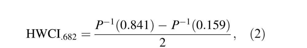 |
where P−1() is the empirical inverse cumulative distribution function of the posterior for CSF or AULCSF. Because CSF was sampled at 19 spatial frequencies, the average HWCI of CSF across 19 spatial frequencies was reported for each individual.
Results
CSFs under three luminance conditions
Figure 2 shows the estimated CSFs and posterior distributions of the AULCSF of several representative observers (S14, S26, S86, and S107) after 50 trials in the L, M, H1, and H2 conditions. As shown in Figure 2, increasing luminance led to increased contrast sensitivity: The posterior distributions of the AULCSF in the L, M, and H conditions were well separated, and the posterior distributions of the AULCSF in the H1 and H2 conditions overlapped with each other.
Figure 2.

Top: Estimated CSFs in the L, M, H1, and H2 conditions of S14, S26, S86, and S107. Shaded regions indicate the 68.2% HWCI. Bottom: Posterior distributions of the estimated AULCSF in the L, M, H1, and H2 conditions of the four observers.
The observations were confirmed by a within-observer analysis of variance based on the data from all 112 observers: Increasing luminance significantly increased the CSF, F(2, 222) = 774.6, p < 0.001. The AULCSFs were significantly different in the L, M, and H conditions, F(2, 222) = 1517.2, p < 0.001, but the CSFs and AULCSFs in the H1 and H2 conditions overlapped and were not different: F(1, 111) = 0.670, p = 0.415; F(1, 111) = 0.646, p = 0.423. These results show that the quick CSF method was able to capture the CSF differences induced by the luminance manipulation and suggested that the method had high test–retest reliability.
Figure 3 shows the AULCSF as a function of background luminance level for all 112 observers. The curves that connect AULCSFs in different luminance conditions generally exhibit an apparent laminar structure: The curves have approximately the same shape but are shifted vertically relative to each other. The pattern of results suggests that changing the mean luminance had similar effects across observers. The mean AULCSF for L, M, H1, and H2 was 1.29 ± 0.15, 1.58 ± 0.13, 1.71 ± 0.12, and 1.71 ± 0.13 log units, respectively. Again, the estimated AULCSFs from the two H conditions were essentially identical. The amount of change across these conditions was calculated as the AULCSF difference between two conditions for each participant. Comparisons that were made included H1–L, M–L, H1–M, and H1–H2. In the rest of this article, the H1–M and H1–L comparisons are denoted as H–M and H–L and are used in further analysis. The mean AULCSF difference for the H–L, M–L, H–M, and H1–H2 comparisons was 0.43 ± 0.10, 0.29 ± 0.07, 0.14 ± 0.07, and 0.00 ± 0.06 log unit, respectively. These mean AULCSF differences served as the “true” magnitude of CSF changes in subsequent power analysis.
Figure 3.

The AULCSF as a function of luminance level for all 112 observers.
Distributions of precision
The precision of a test is inversely proportional to the variability of its measures. A more precise test would deliver a less variable result. The variability of the estimated CSF can be represented by the 68.2% HWCI of the posterior distribution of CSF estimates. Figure 4 shows histograms of the HWCI of the CSFs of all 112 observers in the L, M, H1, and H2 conditions after 50 trials. The mean of the distributions of the HWCI was 0.08 log unit in all conditions. At the same time, the width of the histograms was 0.007 log unit in all conditions. The result suggests that after 50 trials the HWCI values are very stable across observers. For details about HWCI after fewer quick CSF trials, refer to Appendix B.
Figure 4.

Histograms of the 68.2% HWCI of the posterior distribution of CSF in the L, M, H1, and H2 conditions after 50 trials for all 112 observers.
Test–retest reliability
As one measure of test–retest reliability, we computed the mean distances D̄ (see Equation B1 in Appendix B for definition) between the two repeated measures of the CSF measured in the H1 and H2 conditions for all 112 observers. The mean of the D̄ distribution was 0.07 ± 0.03 log unit after 50 trials. The distribution of D̄ (Figure B2) and its relationship with trial number and HWCI (Figure B3) are presented in Appendix B. Generally, HWCI and D̄ are quite comparable.
We also developed a new procedure to assess the test–retest reliability of the quick CSF method from repeated measures in the H1 and H2 conditions. Based on the correlation between repeated measures of contrast sensitivity across all spatial frequencies for each observer, previous assessment of the test–retest reliability of the quick CSF method (Hou et al., 2015; Lesmes et al., 2010) is inadequate because, due to the underlying assumption of the log parabola CSF model, the contrast sensitivities measured by the quick CSF method are highly constrained across spatial frequencies. In order to eliminate such constraint, we developed the following procedure: (a) Randomly divide the 112 observers into 19 groups such that there are six observers in each of the first 18 groups and four observers in the last group; (b) for each of the 19 spatial frequencies, randomly select a group (without replacement) and obtain contrast sensitivities of H1 and H2 at that spatial frequency from the six or four observers in that group; (c) run correlation analysis on the 112 pairs of CSF (H1 and H2) constructed in step 2; and (d) repeat steps 1 to 3 a total of 500 times and calculate the average correlation coefficient.
In this procedure, the sensitivities at difference spatial frequencies were from completely different observers and were not constrained by the truncated log parabola model such that, under the null hypothesis, the baseline correlation between unrelated pairs of CSF would be zero. The average correlation coefficient is plotted as a function of trial number in Figure 5. The average correlation coefficient was 0.751, 0.836, 0.924, and 0.974 after five, 10, 20, and 50 quick CSF trials, respectively. After 15 trials, the average correlation reached 0.9. This result shows that the quick CSF is highly reliable across repeated tests. The correlation coefficients can also be used to estimate the variability of estimated CSF (see Appendix B).
Figure 5.

Average Pearson correlation coefficient as a function of trial number.
Detecting CSF changes in individuals: Sensitivity and specificity
The quick CSF method provides not only a (conventional) point estimate but also the posterior distribution of the estimate of interest that can be exploited to test and detect CSF changes of an individual in different conditions. In this analysis, we focus on detection of AULCSF changes based on the posterior distribution of the AULCSF measured in different luminance conditions for each individual observer.
First, the distribution of AULCSF difference was derived from the posterior distributions of the AULCSFs in the two to-be-compared conditions (i.e., M–L, and H1–H2) of an individual observer (see the bottom row of Figure 2 for the AULCSF distributions at single conditions):
 |
where a and Δa represent AULCSF and AULCSF difference, respectively; pdifference() is the distribution of the AULCSF difference, and p1(·) and p2(·) are the posterior distributions of AULCSF in the two conditions. This posterior inference should be regarded as being conservative (i.e., with greater variance) because it does not reflect the possible a priori correlation of the two AULCSFs. The posterior distributions of the AULCSF difference for H1–H2, H–L, M–L, and H–M after 50 trials of observers S14, S26, S86, and S107 are shown in Figure 6.
Figure 6.

The distribution of the AULCSF difference between conditions after 50 quick CSF trials are plotted in separate panels for observers S14, S26, S86, and S107. The blue curve represents the distribution of the AULCSF difference between H1 and H2. The red, green, and purple curves represent the distribution of the AULCSF difference for H–L, M–L, and H–M, respectively.
The distribution of AULCSF differences between two repeated measures in the same conditions, H1–H2, obtained for each individual, was used as a reference. We assumed that the shape of the distribution of AULCSF difference does not change with its mean. This assumption is reasonable because the HWCIs of the posterior distributions of AULCSF differences between different test conditions were almost the same. The 95% credible interval of the AULCSF difference distribution between H1 and H2 was set as the change criterion. Any AULCSF difference within the criterion was classified as no change, whereas any AULCSF difference outside the criterion was classified as a change.
The concepts of Sensitivity and specificity metrics were used to evaluate the performance of the quick CSF method (Matchar & Orlando, 2007; Rosser, Cousens, Murdoch, Fitzke, & Laidlaw, 2003). Sensitivity is defined as the probability of reporting a change when there is a real condition change. Specificity is defined as the probability of declaring no change when there is no change (i.e., H1–H2). By definition, the specificity corresponding to the 95% criterion credible interval is 95%.
The sensitivity for detecting an AULCSF change for observers S14, S26, S86, and S107 and the average of 112 observers is plotted in Figure 7. Generally, the sensitivity increased with trial number. The average sensitivity for detecting an AULCSF change (0.43 log unit) between the H and L conditions at the individual level was 19.5%, 42.5%, 71.6%, and 97.2% with 5, 10, 20, and 50 quick CSF trials, respectively. The average sensitivity for detecting an AULCSF change (0.29 log unit) between the M and L conditions at the individual level was 19.5%, 32.0%, 45.1%, and 81.0% with 5, 10, 20, and 50 quick CSF trials, respectively. The average sensitivity for detecting an AULCSF change (0.14 log unit) between H and M conditions was 11.0%, 15.6%, 19.5%, and 38.6% with 5, 10, 20, and 50 quick CSF trials, respectively, at the individual level.
Figure 7.

Sensitivities of the quick CSF method in detecting an AULCSF change for observers (a) S14, (b) S26, (c) S86, and (d) S107 as functions of trial number. (e) The average sensitivities across all 112 observers as functions of trial number. Different colors represent the sensitivities of detecting different changes.
Because the width of the criterion region could affect both sensitivity and specificity, we carried out a receiver operating characteristic (ROC) analysis (Swets & Pickett, 1982). Specifically, we varied the change criterion across the credible interval range (0%–100%) and computed the corresponding average sensitivity for the changes of H–L, M–L, and H–M. The average sensitivity can be plotted against 1 − specificity to yield the ROC. The area under the ROC curve provides a measure of the accuracy of correctly classifying change versus no change for the quick CSF method. Figure 8a through c shows the curves after 5, 10, 20, and 50 quick CSF trials.
Figure 8.

The ROC curves for detecting AULCSF change between (a) the H and L conditions, (b) the M and L conditions, and (c) the H and M conditions. The curves in different colors represent results obtained with different numbers of quick CSF trials. (d) Accuracy of the quick CSF method in detecting different AULCSF change between the H and L conditions (red), the M and L conditions (green), and the H and M conditions (blue).
With 50 quick CSF trials, the accuracy of the quick CSF method in detecting AULCSF changes in H–L and M–L at the individual observer level was close to 100% (Figure 8a, b), whereas it was lower in detecting changes in H–M (Figure 8c). In Figure 8d, the accuracy of CSF change detection is plotted as functions of quick CSF trial number for different changes. The accuracy of detecting an AULCSF change (0.43 log unit) between the H and L conditions was 65.6%, 79.3%, 91.4%, and 98.9% with 5, 10, 20, and 50 quick CSF trials, respectively. The accuracy of detecting an AULCSF change (0.29 log unit) between the M and L conditions was 66.3%, 71.3%, 78.4%, and 94.0% with 5, 10, 20, and 50 quick CSF trials, respectively. The average accuracy of detecting an AULCSF change (0.14 log unit) between the H and M conditions was 57.2%, 60.2%, 63.4%, and 76.0% with 5, 10, 20, and 50 quick CSF trials, respectively.
Detecting CSF changes between groups: Statistical power
The large sample size used in the current study made it possible for us to evaluate the performance of the quick CSF method in detecting changes in group mean between two conditions. We conducted an empirical power analysis by using the average effect size of all observers as the true effect size rather than a hypothetical effect size in the conventional power analysis. This way, we were able to provide a realistic assessment of the detectability of group mean changes when the quick CSF method is deployed in the laboratory or clinic.
The empirical power analysis was performed with the following procedure. For a given number N (N = 2, 3, . . . , 112), we randomly selected N observers from the total sample of 112 observers with replacement and performed power analyses for paired t-test based on the observed standard deviation of the AULCSF of the subset of observers. The average effect sizes of AULCSF change (over 112 observers)—0.43, 0.29, and 0.14 for H–L, M–L, and H–M, respectively—were considered as the true effect sizes. The statistical power for detecting AULCSF change for H–L, M–L, and H–M with α = 0.05 was calculated. The procedure was repeated 1,000 times, and the average power was taken as the estimated power of the quick CSF method in detecting respective group mean changes. Figure 9 shows the estimated power as a function of the number of observers and the number of quick CSF trials as heat maps for different changes.
Figure 9.

The power of the quick CSF method to detect group AULCSF changes is presented as functions of the observer and quick CSF trial numbers for changes between (a) the H and L conditions, (b) the M and L conditions, and (c) the H and M conditions.
After 10 quick CSF trials, we needed only 8, 7, and 60 observers to detect an AULCSF change in the H–L, M–L, and H–M comparisons with 95% power, respectively. After 20 trials, we needed only 5, 5, and 20 observers to detect a mean AULCSF change in all comparisons, respectively. After 50 trials, we needed only 4, 4, and 10 observers to detect a mean AULCSF change in all comparisons, respectively.
We can also assess statistical power in terms of the number of trials instead of the number of observers. For example, with 10 observers, we needed 7, 7, and 35 quick CSF trials to detect an AULCSF change in the H–L, M–L, and H–M comparisons with 0.95 power, respectively. With 20 observers, we needed only 5, 4, and 22 trials to detect respective AULCSF changes. With 112 observers, we needed only one, one, and six trials to detect respective AULCSF changes.
We also evaluated the effect size that is required for the quick CSF method to detect a mean AULCSF change for given numbers of observers and trials. We assumed that the distribution of AULCSF differences between the two conditions is Gaussian and that the shape or standard deviation of it does not change with its mean. The former assumption was validated by the Kolmogorov–Smirnov test. The histograms of the AULCSF difference after 50 quick CSF trials for H–L, M–L, H–M, and H1–H2 are shown in Figure 10a, b, c, and d, respectively. One-sample Kolmogorov–Smirnov tests were applied to the AULCSF differences of all observers. The results showed that the distributions of AULCSF changes were normal for all comparisons (all p > 0.05). We used the Brown–Forsythe test for variance equality for the distribution of AULCSF differences in M–L, H–M, and H1–H2 comparisons. There was no difference found in the standard deviation of the AULCSF differences in H1–H2, M–L, and H–M (all p > 0.05 except for trial 1; Figure 11a). It suggests that the standard deviation of the AULCSF difference was independent of the baseline level of AULCSF differences observed between conditions. We calculated the average standard deviation across the three comparisons and plotted it against trial number in Figure 11b. This value was used in the following analyses.
Figure 10.

Histograms of AULCSF difference in comparisons for (a) H1–H2, (b) H–L, (c) M–L, and (d) H–M. These histograms show normality and equal variance.
Figure 11.

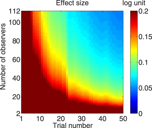
(a) The p value of the Brown–Forsythe test as a function of trial number. All p values > 0.05 except for trial 1, signifying the same standard deviation of the AULCSF difference in all AULCSF comparisons. (b) The empirical standard deviation of population AULCSF difference as a function of trial number. (c) The effect size that can be detected by the quick CSF method with α = 0.05 and power = 0.95 as a joint function of observer and trial numbers.
For any given number of trials, the effect size of change that the quick CSF method can detect with α = 0.05 and power = 0.95 was computed for a given number of observers, N (N = 2, 3, . . . , 112) based on the estimated standard deviation in Figure 11b. In Figure 11c, the effect size is plotted as a function of number of observers and trials. Generally, with more observers and trials, the effect size that is required for the quick CSF method to detect an AULCSF change shrinks. To detect 0.2, 0.1, and 0.05 log unit of AULCSF changes with 20 quick CSF trials, we would need 8, 25, and 93 observers, respectively. To detect the same amounts of difference in 50 trials, only 4, 9, and 28 observers would be needed. With 20 observers, we would need 7, 23, and more than 50 trials to detect 0.2, 0.1, and 0.05 log unit of AULCSF changes, respectively. With 112 observers, we needed only 1, 6, and 15 trials to detect the same amount of difference, respectively. In fact, we could detect a difference of less than 0.025 log unit (6% difference) with 112 observers and 50 trials.
Discussion
In this study, we collected CSFs from 112 college students under three luminance conditions and performed comprehensive analyses on the data to evaluate the performance of the quick CSF method. We evaluated the distribution of the precision of the CSFs obtained from the quick CSF method. The test–retest reliability of the quick CSF method was revisited using an elaborated procedure that was possible only with a large data sample. The test–retest reliability was greater than 0.9 after 15 quick CSF trials and reached 0.974 with 50 trials, which suggests that the quick CSF delivers stable measurements. The rich information contained in the posterior distribution of the CSF measures obtained with the quick CSF method allowed us to test and detect CSF changes on each individual observer. Mild, medium, and large AULCSF changes can be detected with 76.9%, 94.0%, and 98.9% accuracy in 50 quick CSF trials. A power analysis showed that an effect size of 0.025 log unit (6% difference) can be detected with the quick CSF method with 112 observers and 50 trials.
Although we used luminance manipulation to create CSF changes that mimic commonly observed CSF changes in clinical settings, measuring CSF changes in low luminance conditions is especially informative for aging vision due to the prominent loss of sensitivity to high spatial frequency due to age (Derefeldt, Lennerstrand, & Lundh, 1979; Owsley et al., 1983; Sloane, Owsley, & Alvarez, 1988). The dark-adapted CSF is very informative in the diagnosis of AMD (Liu, Wang, & Bedell, 2014). Because there is a substantial loss of parafoveal rod photoreceptors (Curcio, Owsley, & Jackson, 2000) and small-scale, randomly scattered lesions across the macula associated with drusen (Johnson et al., 2003), the retina illumination is attenuated compared with young people. The time course of dark adaptation of both cones and rods in AMD was found to be delayed relative to young people (Owsley et al., 2000; Phipps, Guymer, & Vingrys, 2003). Dark adaptation commonly lasts 30 to 40 min (Hecht, Haig, & Chase, 1937). In order to assess the CSF during the course of dark adaptation, the testing procedure must be as short as possible. The quick CSF method shows promise because it is rapid (10 trials; approximately 2 min) and precise (approximately 0.2 log unit).
Sloane, Owsley, and Jackson (1988) measured contrast sensitivity as a function of luminance and showed that the log sensitivity versus log luminance function had a slope of 0.5 for spatial frequencies ranging from 2 to 4 cpd. In our study, the slope of the log sensitivity versus log luminance function was 0.19 in the same range, and the slope of the AULCSF versus log luminance function was 0.275 (Figure 3). We attribute the discrepancy in the slope for log sensitivity to different testing conditions. Sloane, Owsley, and Jackson (1988) used brief displays and stimuli with a fixed size across all spatial frequencies, whereas we used stimuli that decreased in size as a function of spatial frequency and lasted until response.
Several quick CSF studies on patients with AMD, amblyopia, and glaucoma showed that a similar or slightly greater number of trials (<25%) was required to achieve the same precision on clinical populations as normal subjects, and the test precision did not depend on patients' overall level of visual deficits (Babakhan et al., 2015; Hou et al., 2010; Lesmes et al., 2012, 2013; Ramulu et al., 2015; Rosen et al., 2015). Because only normal participants were included in this study, the performance of the quick CSF method in clinical populations should be further examined in future studies.
We conducted another statistical power analysis with the conservative assumption that the standard deviation of AULCSF changes in patients is twice that of the normal observers in the current study. The results are shown in Figure 12. To detect 0.2 and 0.1 log unit of AULCSF changes with 20 quick CSF trials, we would need to run 25 and 93 observers, respectively. To detect the same amounts of difference in 50 trials, 9 and 28 observers would be needed. With 20 observers, we would need 23 and more than 50 trials to detect 0.2 and 0.1 log unit of difference, respectively. With 112 observers, we needed only 6 and 15 trials to detect the same amount of difference, respectively. The effect size changes with trial and observer numbers in a way that is very similar to that of the normal group.
Figure 12.
The effect size that can be detected by the quick CSF method with α = 0.05 and power = 0.95 as a joint function of both observer and trial numbers for a group having AULCSF changes with 2 × standard deviation.
The individual-level CSF change detection method developed in the current study was based on the posterior distribution of AULCSF, which is a summary measure of CSF. Patients may exhibit significant CSF deficits in specific spatial frequency regions due to different morphological or pathological characteristics (Huang, Tao, Zhou, & Lu, 2007; Midena et al., 1997; Regan, 1991). There are at least two ways the performance of quick CSF in detecting CSF changes could potentially be improved: (a) Replace the posterior distribution of AULCSF with the high dimensional posterior distribution of all CSF parameters or posterior distributions of AULCSF in low, medium, and high frequency regions and (b) use machine learning techniques to select the most informative features among different CSF characteristics (e.g., cutoff, maximum sensitivity, CSF acuity, CSF parameters).
In summary, our study demonstrates that the quick CSF method is very precise and reliable at detecting changes in contrast sensitivity. It showed excellent statistical power in detecting CSF changes at the group level. At the individual level, the quick CSF demonstrated excellent power in detecting medium to large visual losses (94% accuracy) but only moderate power in detecting more subtle functional deficits in single tests (76% accuracy). For these subtle deficits, repeated testing will likely be needed to increase statistical power. Taken together, the methods introduced and discussed in this article show early promise as tools for monitoring the progression of vision loss in eye disease or its remediation with treatment. More studies are needed to evaluate how effectively these tools can reduce the sample sizes, lengths, and costs of clinical trials.
Supplementary Material
Acknowledgments
This study was supported by the National Eye Institute (Grant EY021553 to ZLL) and by the National Institute of Mental Health (Grant MH093838 to JM and MP).
Commercial relationships: LL and ZLL own intellectual property interests on quick CSF technology and financial interests in Adaptive Sensory Technology, Inc. LL holds employment at Adaptive Sensory Technology, Inc.
Corresponding author: Zhong-Lin Lu.
Email: lu.535@osu.edu.
Address: Department of Psychology, The Ohio State University, Columbus, OH, USA.
Appendix A: Quick CSF algorithm
The quick CSF used the following steps to estimate τ(f) (Lesmes et al., 2010):
1. Define a CSF functional form.
τ(f) is the reciprocal of contrast sensitivity S(f),  which is described by the truncated log parabola with four parameters (Lesmes et al., 2010; Watson & Ahumada, 2005; Figure A1):
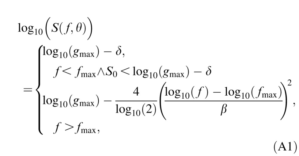 |
where θ = (gmax, fmax, β, δ) represents the four CSF parameters: peak gain (gmax), peak spatial frequency (fmax), bandwidth at half height (β, in octaves), and low frequency truncation level (δ).
2. Define the stimulus and parameter spaces. The application of Bayesian adaptive inference requires two basic components: (a) a prior probability distribution, p(θ), defined over a four-dimensional space of CSF parameters θ, and (b) a two-dimensional space of possible letter stimuli with contrast c and spatial frequency f. In our simulation study, the ranges of possible CSF parameters were 2 to 2,000 for peak gain, 0.2 to 20 cpd for peak frequency, 1 to 9 octaves for bandwidth, and 0.02 to 2 for truncation. The ranges for possible grating stimuli were 0.2% to 100% for contrast c and 1.19 to 30.95 cpd for frequency f. Both parameter and stimuli spaces were sampled evenly in log units.
Figure A1.

The quick CSF method adopts a four-parameter truncated log parabolic functional form to describe the shape of the CSF (a) and selects the optimal test stimulus in each trial in the two-dimensional contrast and spatial frequency space. The history of stimulus selection of 300 quick CSF trials in a simulation study is shown in panel b. The coordinates of the “x” symbols represent the spatial frequency and contrast of the test stimuli.
3. Priors. Before the beginning of the experiment, an initial prior, pt = 0(θ), which represents the knowledge about the observer's CSF before any data are collected, was defined by a hyperbolic secant function with the best guess of parameters θi,guess and width of θi,confidence for i = 1, 2, 3, and 4 (King-Smith & Rose, 1997; Lesmes et al., 2010):
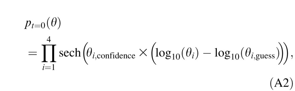 |
where sech(x) = 2/(ex + e−x); θi = gmax, fmax, β, and δ for i = 1, 2, 3, and 4, respectively; θi,guess = 100, 2, 3, and 0.5 for i = 1, 2, 3, and 4, respectively; and θi,confidence = 2.48, 3.75, 7.8, and 3.12 for i = 1, 2, 3, and 4, respectively.
4. Bayesian adaptive inference. In trial t, the observer makes three responses:  = “correct” or “incorrect” corresponding to three letters xi = (ci, f ) with contrast ci and spatial frequency f, where i = 1, 2, and 3 represents the ith letter from left to right. After observer's (three) responses are collected in trial t, knowledge about CSF parameters p(θ) is updated. The outcome of trial t is incorporated into a Bayesian inference step that updates the knowledge about CSF parameters pt−1(θ) prior to trial t:
 |
where  is the posterior distribution of parameter vector θ after obtaining a response rx at trial t;
  is the percentage correct psychometric function given stimulus xi; and
  ; pt−1(θ) is our prior about θ before trial t, which is also the posterior in trial t − 1.
5. Stimulus search. To increase the quality of the evidence obtained on each trial, the quick CSF calculates the expected information gain for all possible stimuli x:
 |
where h(p) = −p log(p) − (1 − p)log(1 − p) is the information entropy of the distribution p. Before each trial, we find out the candidate stimuli that correspond to the top 10% of the expected information gain over the entire stimulus space. Then we randomly pick one among those candidates as xt = (c, f) for presentation. In this way, the quick CSF avoids large regions of the stimulus space that are not likely to provide useful information to the current knowledge about θ. To improve observers' experience in CSF testing, two additional letters with higher contrasts are presented alongside the optical test letter xt. From left to right, their contrasts are 4c, 2c, and c, respectively. The maximum contrast is capped at 90%. Their spatial frequency is f.
6. Reiteration and stopping rule. The quick CSF procedure reiterates steps 4 and 5 until 50 trials have been run.
7. Analysis. After step 6, we obtain the posterior distribution in numerical form of CSF parameters pt(θ) (see Figure A2 for the marginal prior and posterior distributions for the four CSF parameters). A resampling procedure is used that samples directly from the posterior distributions of the CSF parameters and generates the CSF estimates (i.e., CSF and AULCSF) based on all the CSF samples. The procedure automatically takes into account the covariance structure of the CSF parameters in the posterior distribution and allows us to compute the credible interval of the estimates derived from CSF functions.
Figure A2.
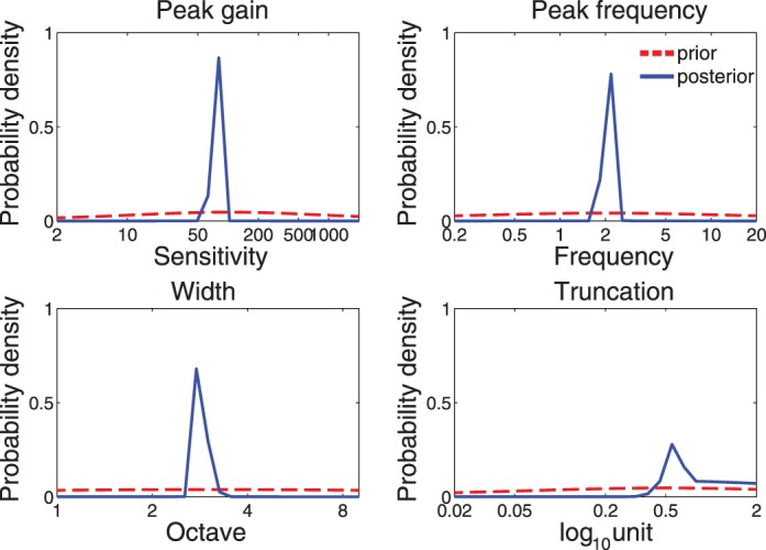
The marginal distributions of four parameters before (prior: red) and after (posterior: blue) measurement. The plot was based on the simulation of a single quick CSF run with 100 trials.
Appendix B: Detailed precision analysis
Figure B1 shows histograms of the HWCI of the CSFs of all 112 observers in the L, M, H1, and H2 conditions after five, 10, 20, and 50 trials. The mean of the distributions of the HWCI was 0.36, 0.20, 0.13, and 0.08 after five, 10, 20, and 50 trials, respectively, in the L condition; 0.36, 0.21, 0.13, and 0.08 in the M condition; 0.32, 0.20, 0.13, and 0.08 in the H1 condition; and 0.34, 0.19, 0.13, and 0.08 in the H2 condition (all in log units). The HWCIs of the CSFs in the four conditions were about the same. At the same time, the width of all the histograms narrowed as trial number increased: The standard deviation of HWCI decreased by an order of magnitude from 0.07 to 0.007, 0.075 to 0.007, 0.067 to 0.007, and 0.071 to 0.007 in the L, M, H1, and H2 conditions, respectively, as trial number increased from 1 to 50. The result suggests that the confidence of the estimated HWCI increases as trial number increases. Although they varied widely across different observers at trial 1, the HWCI values stabilized across observers after 10 trials.
Figure B1.

Histograms of the 68.2% HWCI of the posterior distribution of CSF in the L, M, H1, and H2 conditions after 5, 10, 20, and 50 trials for all 112 observers.
The variability of CSF estimates can also be computed in another way—that is, the standard deviation of the estimated CSFs in repeated measurements (Hou et al., 2015). Given that there were only two repeated CSF measurements in the H condition, we computed the mean distance between two CSF measures for each participant:
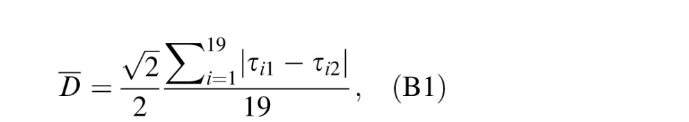 |
where τi1 and τi2 are estimated CSFs (i.e., posterior means) at the ith (i = 1, 2, . . . , 19) spatial frequency in the H1 and H2 conditions, respectively.  is a correction coefficient to make the distance essentially the same as the standard deviation of estimated CSF in two repeated measurements.
Figure B2 shows histograms of the mean distances D̄ between the two repeated measures of the CSF measured in the H1 and H2 conditions after 5, 10, 20, and 50 trials for all 112 observers. The mean of the distribution of D̄ was 0.22, 0.16, 0.11, and 0.07 log unit after 5, 10, 20, and 50 trials, respectively. The width of the distributions narrowed as trial number increased: The standard deviation of the mean distance decreased from 0.23 to 0.03 as trial number increased from 1 to 50. It should be noted that the variability of the estimated standard deviation was greater than that of HWCI. This is likely because there were only two repeated measurements of the CSF in the H condition. Running more repeated tests would reduce this variability.
Figure B2.

Histograms of the mean distance, as defined in Equation B1, of the two estimated CSFs in the H1 and H2 conditions after 5, 10, 20, and 50 trials for all 112 observers.
Figure B3 shows the average HWCI across subjects (in the H1 condition) and average mean distance as functions of trial number. Both measures of variability decreased quickly with number of trials. Most importantly, the two measures of variability were very similar, suggesting that the HWCI from a single quick CSF assessment is an adequate estimate that reflects the precision of the quick CSF method.
Figure B3.
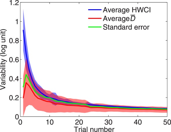
The average (over observers) HWCI (blue) and mean distance (red) of measured CSF are plotted as functions of trial number. The shaded area indicates ±1 SD for HWCI. The standard error of the estimated CSF is also plotted in green.
The variability of the estimated CSF can also be derived from the correlation coefficient (Lord & Novick, 1968):
 |
where SE is the standard error of the estimated CSF, SDsample is the standard deviation of the pooled CSFs of all observers in the H1 and H2 conditions, and r is the average correlation coefficient between the two repeated measures. The standard error is also plotted as a function of trial number in Figure B3. The standard error is virtually identical to the other two variability measures.
Contributor Information
Fang Hou, Email: hou.130@osu.edu.
Luis Andres Lesmes, Email: luis.lesmes@adaptivesensorytech.com.
Woojae Kim, Email: wjaekim.1124@gmail.com.
Hairong Gu, Email: nonlosing@gmail.com.
Mark A. Pitt, Email: pitt.2@osu.edu.
Jay I. Myung, Email: myung.1@osu.edu.
Zhong-Lin Lu, lu.535@osu.edu, lobes.osu.edu.
References
- Alexander, K. R.,, Xie W.,, Derlacki D. J. (1994). Spatial-frequency characteristics of letter identification. Journal of the Optical Society of America A: Optics, Image Science, and Vision, 11, 2375–2382. [DOI] [PubMed] [Google Scholar]
- American National Standards Institute. (2001). American National Standard for Ophthalmics—Multifocal intraocular lenses. Fairfax, VA: Optical Laboratories Association. [Google Scholar]
- Applegate R. A.,, Howland H. C.,, Sharp R. P.,, Cottingham A. J.,, Yee R. W. (1998). Corneal aberrations and visual performance after radial keratotomy. Journal of Refractive Surgery, 14, 397–407. [DOI] [PubMed] [Google Scholar]
- Arden G. B.,, Jacobson J. J. (1978). A simple grating test for contrast sensitivity: Preliminary results indicate value in screening for glaucoma. Investigative Ophthalmology & Visual Science, 17, 23–32. [PubMed] [Article] [PubMed] [Google Scholar]
- Babakhan L.,, Parfenova A.,, Ha K.,, Maeda R.,, Thurman S.,, Seitz A. R.,, Davey P. G. (2015). Repeatability of measurements obtained using the quick CSF method. ARVO Meeting Abstracts, 56, 3901-D0043. [Google Scholar]
- Barnes R. M.,, Gee L.,, Taylor S.,, Briggs M. C.,, Harding S. P. (2004). Outcomes in verteporfin photodynamic therapy for choroidal neovascularisation—“Beyond the TAP study.” Eye (London), 18, 809–813. [DOI] [PubMed] [Google Scholar]
- Bellmann C.,, Unnebrink K.,, Rubin G. S.,, Miller D.,, Holz F. G. (2003). Visual acuity and contrast sensitivity in patients with neovascular age-related macular degeneration. Results from the Radiation Therapy for Age-Related Macular Degeneration (RAD-) Study. Graefe's Archive for Clinical and Experimental Ophthalmology, 241, 968–974. [DOI] [PubMed] [Google Scholar]
- Bradley A.,, Hook J.,, Haeseker J. (1991). A comparison of clinical acuity and contrast sensitivity charts: Effect of uncorrected myopia. Ophthalmic and Physiological Optics, 11, 218–226. [PubMed] [Google Scholar]
- Buhren J.,, Terzi E.,, Bach M.,, Wesemann W.,, Kohnen T. (2006). Measuring contrast sensitivity under different lighting conditions: Comparison of three tests. Optometry & Vision Science, 83, 290–298. [DOI] [PubMed] [Google Scholar]
- Chung S. T.,, Legge G. E.,, Tjan B. S. (2002). Spatial-frequency characteristics of letter identification in central and peripheral vision. Vision Research, 42, 2137–2152. [DOI] [PubMed] [Google Scholar]
- Clayton D.,, Hills M. (1993). Statistical models in epidemiology. Oxford, UK: Oxford University Press. [Google Scholar]
- Curcio C. A.,, Owsley C.,, Jackson G. R. (2000). Spare the rods, save the cones in aging and age-related maculopathy. Investigative Ophthalmology & Visual Science, 41, 2015–2018. [PubMed] [Article] [PubMed] [Google Scholar]
- Derefeldt G.,, Lennerstrand G.,, Lundh B. (1979). Age variations in normal human contrast sensitivity. Acta Ophthalmologica (Copenhagen), 57, 679–690. [DOI] [PubMed] [Google Scholar]
- Dorr M.,, Lesmes L. A.,, Lu Z. L.,, Bex P. J. (2013). Rapid and reliable assessment of the contrast sensitivity function on an iPad. Investigative Ophthalmology & Visual Science, 54, 7266–7273. [PubMed] [Article] [DOI] [PMC free article] [PubMed] [Google Scholar]
- Gepshtein S.,, Lesmes L. A.,, Albright T. D. (2013). Sensory adaptation as optimal resource allocation. Proceedings of the National Academy of Sciences, USA, 110, 4368–4373. [DOI] [PMC free article] [PubMed] [Google Scholar]
- Ginsburg A. P. (1981). Spatial filtering and vision: Implications for normal and abnormal vision. Proenz L., Enoch J., Jampolsky A. (Eds.) Clinical applications of visual psychophysics (pp 70–106). Cambridge, UK: Cambridge University Press. [Google Scholar]
- Ginsburg, A. P. (2003). Contrast sensitivity and functional vision. International Ophthalmology Clinics, 43 (2), 5–15. [DOI] [PubMed] [Google Scholar]
- Harvey L. O.,, Jr. (1997). Efficient estimation of sensory thresholds with ML-PEST. Spatial Vision, 11, 121–128. [DOI] [PubMed] [Google Scholar]
- Haymes S. A.,, Roberts K. F.,, Cruess A. F.,, Nicolela M. T.,, LeBlanc R. P.,, Ramsey M. S.,, Artes P. H. (2006). The letter contrast sensitivity test: Clinical evaluation of a new design. Investigative Ophthalmology & Visual Science, 47, 2739–2745. [PubMed] [Article] [DOI] [PubMed] [Google Scholar]
- Hecht S.,, Haig C.,, Chase A. M. (1937). The influence of light adaptation on subsequent dark adaptation of the eye. Journal of General Physiology, 20, 831–850. [DOI] [PMC free article] [PubMed] [Google Scholar]
- Hess R. F. (1981). Application of contrast-sensitivity techniques to the study of functional amblyopia. Proenz L., Enoch J., Jampolsky A. (Eds.) Clinical applications of visual psychophysics (pp 11–41). Cambridge, UK: Cambridge University Press. [Google Scholar]
- Hess, R. F.,, Howell E. R. (1977). The threshold contrast sensitivity function in strabismic amblyopia: Evidence for a two type classification. Vision Research, 17, 1049–1055. [DOI] [PubMed] [Google Scholar]
- Hohberger B.,, Laemmer R.,, Adler W.,, Juenemann A. G.,, Horn F. K. (2007). Measuring contrast sensitivity in normal subjects with OPTEC 6500: Influence of age and glare. Graefe's Archive for Clinical and Experimental Ophthalmology, 245, 1805–1814. [DOI] [PubMed] [Google Scholar]
- Hou F.,, Huang C.-B.,, Lesmes L.,, Feng L.-X.,, Tao L.,, Zhou Y.-F.,, Lu Z. L. (2010). qCSF in clinical application: Efficient characterization and classification of contrast sensitivity functions in amblyopia. Investigative Ophthalmology & Visual Science, 51, 5365–5377. [PubMed] [Article] [DOI] [PMC free article] [PubMed] [Google Scholar]
- Hou F.,, Lesmes L.,, Bex P.,, Dorr M.,, Lu Z. L. (2015). Using 10AFC to further improve the efficiency of the quick CSF method. Journal of Vision, 15 (9): 18 1–18, doi:10.1167/15.9.2 [PubMed] [Article] [DOI] [PMC free article] [PubMed] [Google Scholar]
- Hou F.,, Lu Z. L.,, Huang C. B. (2014). The external noise normalized gain profile of spatial vision. Journal of Vision, 14 (13): 18 1–14, doi:10.1167/14.13.9 [PubMed] [Article] [DOI] [PMC free article] [PubMed] [Google Scholar]
- Huang C.,, Tao L.,, Zhou Y.,, Lu Z. L. (2007). Treated amblyopes remain deficient in spatial vision: A contrast sensitivity and external noise study. Vision Research, 47, 22–34. [DOI] [PubMed] [Google Scholar]
- Jia W.,, Yan F.,, Hou F.,, Lu Z.-L.,, Huang C.-B. (2014). qCSF in clinical applications: Efficient characterization and classification of contrast sensitivity functions in aging. ARVO Meeting Abstracts, 55, 762. [Google Scholar]
- Jindra L. F.,, Zemon V. (1989). Contrast sensitivity testing: A more complete assessment of vision. Journal of Cataract & Refractive Surgery, 15, 141–148. [DOI] [PubMed] [Google Scholar]
- Johnson P. T.,, Lewis G. P.,, Talaga K. C.,, Brown M. N.,, Kappel P. J.,, Fisher S. K.,, Johnson L. V. (2003). Drusen-associated degeneration in the retina. Investigative Ophthalmology & Visual Science, 44, 4481–4488. [PubMed] [Article] [DOI] [PubMed] [Google Scholar]
- Kalia A.,, Lesmes L. A.,, Dorr M.,, Gandhi T.,, Chatterjee G.,, Ganesh S.,, Sinha P. (2014). Development of pattern vision following early and extended blindness. Proceedings of the National Academy of Sciences, USA, 111, 2035–2039. [DOI] [PMC free article] [PubMed] [Google Scholar]
- Kelly D. H.,, Savoie R. E. (1973). A study of sine-wave contrast sensitivity by two psychophysical methods. Perception & Psychophysics, 14, 313–318. [Google Scholar]
- Keltner J. L.,, Johnson C. A.,, Quigg J. M.,, Cello K. E.,, Kass M. A.,, Gordon M. O. (2000). Confirmation of visual field abnormalities in the Ocular Hypertension Treatment Study. Ocular Hypertension Treatment Study Group. Archives of Ophthalmology, 118, 1187–1194. [DOI] [PubMed] [Google Scholar]
- King-Smith P. E.,, Rose D. (1997). Principles of an adaptive method for measuring the slope of the psychometric function. Vision Research, 37, 1595–1604. [DOI] [PubMed] [Google Scholar]
- Kleiner M.,, Brainard D.,, Pelli D. (2007). What's new in Psychtoolbox-3? [Abstract]. Perception, 36, 14. [Google Scholar]
- Kleiner R. C.,, Enger C.,, Alexander M. F.,, Fine S. L. (1988). Contrast sensitivity in age-related macular degeneration. Archives of Ophthalmology, 106, 55–57. [DOI] [PubMed] [Google Scholar]
- Kooijman A. C.,, Stellingwerf N.,, van Schoot E. A. J.,, Cornelissen F. W.,, van der Wildt G. J. (1994). Groningen edge contrast chart (GECKO) and glare measurements. Kooijman A. C., Looijestijn P. L., Welling J. A., van der Wildt G. J. (Eds.) Low vision (pp 101–110). Lansdale, PA: IOS Press. [Google Scholar]
- Lee, T. H.,, Baek J.,, Lu Z. L.,, Mather M. (2014). How arousal modulates the visual contrast sensitivity function. Emotion, 14, 978–984. [DOI] [PMC free article] [PubMed] [Google Scholar]
- Lesmes L.,, Wallis J.,, Jackson M. L.,, Bex P. (2013). The reliability of the quick CSF method for contrast sensitivity assessment in low vision. Investigative Ophthalmology & Visual Science, 54, 2762 [Abstract] [Google Scholar]
- Lesmes L.,, Wallis J.,, Lu Z.-L.,, Jackson M. L.,, Bex P. J. (2012). Clinical application of a novel contrast sensitivity test to a low vision population: The quick CSF method. ARVO Meeting Abstracts, 53, 4358. [Google Scholar]
- Lesmes L. A.,, Lu Z.-L.,, Baek J.,, Albright T. D. (2010). Bayesian adaptive estimation of the contrast sensitivity function: The quick CSF method. Journal of Vision, 10 (3): 18 1–21, doi:10.1167/10.3.17 [PubMed] [Article] [DOI] [PMC free article] [PubMed] [Google Scholar]
- Liu L.,, Wang Y. Z.,, Bedell H. E. (2014). Visual-function tests for self-monitoring of age-related macular degeneration. Optometry & Vision Science, 91, 956–965. [DOI] [PubMed] [Google Scholar]
- Lord F. N.,, Novick M. R. (1968). Statistical theories of mental test scores. Reading, MA: Addison-Wesley. [Google Scholar]
- Marmor M. F. (1981). Contrast sensitivity and retinal disease. Annals of Ophthalmology, 13, 1069–1071. [PubMed] [Google Scholar]
- Marmor M. F. (1986). Contrast sensitivity versus visual acuity in retinal disease. British Journal of Ophthalmology, 70, 553–559. [DOI] [PMC free article] [PubMed] [Google Scholar]
- Marmor M. F.,, Gawande A. (1988). Effect of visual blur on contrast sensitivity. Clinical implications. Ophthalmology, 95, 139–143. [DOI] [PubMed] [Google Scholar]
- Matchar D. B.,, Orlando L. A. (2007). The relationship between test and outcome. Price C. P. (Ed.) Evidence-based laboratory medicine: Principles, practice and outcomes (2nd ed., 53–66). Washington, DC: AACC Press. [Google Scholar]
- McAnany, J. J.,, Alexander K. R. (2006). Contrast sensitivity for letter optotypes vs. gratings under conditions biased toward parvocellular and magnocellular pathways. Vision Research, 46, 1574–1584. [DOI] [PubMed] [Google Scholar]
- Midena E.,, DegliAngeli C., Blarzino M. C.,, Valenti M.,, Segato T. (1997). Macular function impairment in eyes with early age-related macular degeneration. Investigative Ophthalmology & Visual Science, 38, 469–477. [PubMed] [Article] [PubMed]
- Montes-Mico R.,, Charman W. N. (2001). Choice of spatial frequency for contrast sensitivity evaluation after corneal refractive surgery. Journal of Refractive Surgery, 17, 646–651. [DOI] [PubMed] [Google Scholar]
- Montes-Mico R.,, Ferrer-Blasco T. (2001). Contrast sensitivity function in children: Normalized notation for the assessment and diagnosis of diseases. Documenta Ophthalmologica, 103, 175–186. [DOI] [PubMed] [Google Scholar]
- O'Donoghue L.,, Rudnicka A. R.,, McClelland J. F.,, Logan N. S.,, Saunders K. J. (2012). Visual acuity measures do not reliably detect childhood refractive error—An epidemiological study. PLoS ONE, 7 (3), e34441. [DOI] [PMC free article] [PubMed] [Google Scholar]
- Onal S.,, Yenice O.,, Cakir S.,, Temel A. (2008). FACT contrast sensitivity as a diagnostic tool in glaucoma: FACT contrast sensitivity in glaucoma. International Ophthalmology, 28, 407–412. [DOI] [PubMed] [Google Scholar]
- Oshika T.,, Okamoto C.,, Samejima T.,, Tokunaga T.,, Miyata K. (2006). Contrast sensitivity function and ocular higher-order wavefront aberrations in normal human eyes. Ophthalmology, 113, 1807–1812. [DOI] [PubMed] [Google Scholar]
- Owsley C. (2003). Contrast sensitivity. Ophthalmology Clinics of North America, 16, 171–177. [DOI] [PubMed] [Google Scholar]
- Owsley C.,, Jackson G. R.,, Cideciyan A. V.,, Huang Y.,, Fine S. L.,, Ho A. C.,, Jacobson S. G. (2000). Psychophysical evidence for rod vulnerability in age-related macular degeneration. Investigative Ophthalmology & Visual Science, 41, 267–273. [PubMed] [Article] [PubMed] [Google Scholar]
- Owsley C.,, Sekuler R.,, Siemsen D. (1983). Contrast sensitivity throughout adulthood. Vision Research, 23, 689–699. [DOI] [PubMed] [Google Scholar]
- Pesudovs K.,, Hazel C. A.,, Doran R. M.,, Elliott D. B. (2004). The usefulness of Vistech and FACT contrast sensitivity charts for cataract and refractive surgery outcomes research. British Journal of Ophthalmology, 88, 11–16. [DOI] [PMC free article] [PubMed] [Google Scholar]
- Phipps J. A.,, Guymer R. H.,, Vingrys A. J. (2003). Loss of cone function in age-related maculopathy. Investigative Ophthalmology & Visual Science, 44, 2277–2283. [PubMed] [Article] [DOI] [PubMed] [Google Scholar]
- Ramulu P.,, Dave P.,, Friedman D. (2015). Precision of contrast sensitivity testing in glaucoma. ARVO Meeting Abstracts, 56, 2225-B0078. [Google Scholar]
- Regan D. (1991). Spatiotemporal abnormalities of vision in patients with multiple sclerosis. Regan D. (Ed.) Spatial vision (pp 239–249). Boca Raton, FL: CRC Press. [Google Scholar]
- Reynaud, A.,, Tang Y.,, Zhou Y.,, Hess R. (2014). A unified framework and normative dataset for second-order sensitivity using the quick contrast sensitivity function (qCSF). Journal of Vision, 14 (10): 1428, doi:10.1167/14.10.1428 [Abstract] [DOI] [PubMed] [Google Scholar]
- Richman J.,, Lorenzana L. L.,, Lankaranian D.,, Dugar J.,, Mayer J.,, Wizov S. S.,, Spaeth G. L. (2010). Importance of visual acuity and contrast sensitivity in patients with glaucoma. Archives of Ophthalmology, 128, 1576–1582. [DOI] [PubMed] [Google Scholar]
- Rosen R.,, Jayaraj J.,, Bharadwaj S. R.,, Weeber H. A.,, Van der Mooren M.,, Piers P. A. (2015). Contrast sensitivity in patients with macular degeneration. ARVO Meeting Abstracts, 56, 2224-B0077. [Google Scholar]
- Rosén R.,, Lundström L.,, Venkataraman A. P.,, Winter S.,, Unsbo P. (2014). Quick contrast sensitivity measurements in the periphery. Journal of Vision, 14 (8): 18 1–10, doi:10.1167/14.8.3 [PubMed] [Article] [DOI] [PubMed] [Google Scholar]
- Rosser D. A.,, Cousens S. N.,, Murdoch I. E.,, Fitzke F. W.,, Laidlaw D. A. (2003). How sensitive to clinical change are ETDRS logMAR visual acuity measurements? Investigative Ophthalmology & Visual Science, 44, 3278–3281. [PubMed] [Article] [DOI] [PubMed] [Google Scholar]
- Shandiz J. H.,, Nourian A.,, Hossaini M. B.,, Moghaddam H. O.,, Yekta A. A.,, Sharifzadeh L.,, Marouzi P. (2010). Contrast sensitivity versus visual evoked potentials in multiple sclerosis. Journal of Ophthalmic & Vision Research, 5, 175–181. [PMC free article] [PubMed] [Google Scholar]
- Sloane M. E.,, Owsley C.,, Alvarez S. L. (1988). Aging, senile miosis and spatial contrast sensitivity at low luminance. Vision Research, 28, 1235–1246. [DOI] [PubMed] [Google Scholar]
- Sloane M. E.,, Owsley C.,, Jackson C. A. (1988). Aging and luminance-adaptation effects on spatial contrast sensitivity. Journal of the Optical Society of America A, 5, 2181–2190. [DOI] [PubMed] [Google Scholar]
- Swets J. A.,, Pickett R. M. (1982). Evaluation of diagnostic systems: Methods from signal detection theory. New York, NY: Academic Press. [Google Scholar]
- Tyler C. W. (1997). Colour bit-stealing to enhance the luminance resolution of digital displays on a single pixel basis. Spatial Vision, 10, 369–377. [DOI] [PubMed] [Google Scholar]
- van Gaalen K. W.,, Jansonius N. M.,, Koopmans S. A.,, Terwee T.,, Kooijman A. C. (2009). Relationship between contrast sensitivity and spherical aberration: Comparison of 7 contrast sensitivity tests with natural and artificial pupils in healthy eyes. Journal of Cataract & Refractive Surgery, 35, 47–56. [DOI] [PubMed] [Google Scholar]
- Watson A. B.,, Ahumada A. J.,, Jr. (2005). A standard model for foveal detection of spatial contrast. Journal of Vision, 5 (9): 18 717–740, doi:10.1167/5.9.6 [PubMed] [Article] [DOI] [PubMed] [Google Scholar]
- Yenice O.,, Onal S.,, Incili B.,, Temel A.,, Afsar N.,, Tanridag T. (2007). Assessment of spatial-contrast function and short-wavelength sensitivity deficits in patients with migraine. Eye, 21, 218–223. [DOI] [PubMed] [Google Scholar]
Associated Data
This section collects any data citations, data availability statements, or supplementary materials included in this article.