Measuring embeddedness: Hierarchical scale‐dependent information exchange efficiency of the human brain connectome

Abstract

This article presents a novel approach for understanding information exchange efficiency and its decay across hierarchies of modularity, from local to global, of the structural human brain connectome. Magnetic resonance imaging techniques have allowed us to study the human brain connectivity as a graph, which can then be analyzed using a graph‐theoretical approach. Collectively termed brain connectomics, these sophisticated mathematical techniques have revealed that the brain connectome, like many networks, is highly modular and brain regions can thus be organized into communities or modules. Here, using tractography‐informed structural connectomes from 46 normal healthy human subjects, we constructed the hierarchical modularity of the structural connectome using bifurcating dendrograms. Moving from fine to coarse (i.e., local to global) up the connectome's hierarchy, we computed the rate of decay of a new metric that hierarchically preferentially weighs the information exchange between two nodes in the same module. By computing “embeddedness”‐the ratio between nodal efficiency and this decay rate, one could thus probe the relative scale‐invariant information exchange efficiency of the human brain. Results suggest that regions that exhibit high embeddedness are those that comprise the limbic system, the default mode network, and the subcortical nuclei. This supports the presence of near‐decomposability overall yet relative embeddedness in select areas of the brain. The areas we identified as highly embedded are varied in function but are arguably linked in the evolutionary role they play in memory, emotion and behavior. Hum Brain Mapp 36:3653–3665, 2015. © 2015 Wiley Periodicals, Inc.

INTRODUCTION

Magnetic resonance imaging techniques have allowed us to study the human brain both functionally and structurally. Complex interactions between different regions of the brain have necessitated the development and growth of the field of connectomics. The brain connectome is typically mathematically represented using connectivity matrices to describe the interaction among different brain regions. Most current connectome study designs involve the computation of summary statistics on a global or nodal level [Guimera and Amaral, 2005; Sporns et al., 2005]. Additionally, evidence suggests that brain regions are organized into modules, with several key regions of the brain serving as hubs that act as relay centers globally [Colizza et al., 2006; Sporns et al., 2007].

In one of the first attempts to quantify a node's “hubness” in a network [Guimera and Amaral, 2005], after determining the community structure, all nodes had the within‐module degree z and the participation coefficient computed. The within‐module degree (z‐score) is defined as $z_i={(\kappa }_i‐{\overline{\kappa }}_{s_i})/{\sigma }_{{\kappa }_{s_i}}$ where ${\kappa }_i$ is the number of links of node i to other nodes in its module ${ s}_i$, ${\overline{\kappa }}_{s_i}$ is the average of $\kappa$ over all the nodes in $s_i$, and ${\sigma }_{{\kappa }_{s_i}}$ is the standard deviation. The participation coefficient is defined as $P_i=1-{\sum }_{s=1}^{N_M}{\left({\kappa }_{is}/{\kappa }_i\right)}^2$ with ${\kappa }_{\mathrm{i}\mathrm{s}}$ indicating the number of links node i has to nodes in any module s (P values are between 0 and 1, with higher values indicating more links to nodes in other module). A node is said to be a global connector hub if its within‐module degree z‐score is >2.5 and its participation coefficient >0.3.

In brain connectomics, researchers have also adopted similar classification schemes. For example, in [Meunier et al., 2009] the authors demonstrated the existence of hierarchical modular organization (i.e., the ubiquitous property of “near‐decomposability” according to Simon's theory on complex systems; [Fisher, 1961; Simon, 1965; Simon and Ando, 1961]) in human brain resting state functional networks, and proceeded to classify the roles of a node based on various combinations of cut‐off values of within‐module degree z‐score and participation coefficient.

However, here we argue such an approach has two main disadvantages. First, these cut‐off values are ultimately arbitrarily determined and categorical, and thus do not necessarily reflect the complexity and the continuous nature of brain connectivity (e.g., for a non‐hub node, it is classified as ultra‐peripheral if its participation coefficient is less than 0.05, peripheral if between 0.05 and 0.62, connector if between 0.62 and 0.80, and kinless if between 0.80 and 1.0). Second, despite the hierarchical nature of the human connectome, within‐module degree z scores and participation coefficients are still defined after restricting to a specific modular hierarchy, and thus they do not properly capture the potential scale‐dependent nature of a node's role in the network as a whole. In this study, we thus seek to address these issues by proposing a new approach to collectively probe the scale‐dependence of information transfer across all levels of modular hierarchy, without resorting to arbitrary thresholding, binning, or binarization of scalar‐valued datapoints.

In a different yet related context, there have been substantial research efforts exploring topological organizations of neuroanatomy corresponding to the brain's functional “gradients,” for example, how the “ventral” emotional processing system interacts with the “dorsal” executive processing system [Catani et al., 2013; Iordan et al., 2013]. Along these two converging lines, we posit that the novel approach presented in this article would yield results that not only are consistent with these known neuroanatomical topological organizations or “gradients,” but also provide additional insights into the underpinnings of these topologies. In this sense, through acknowledgement and measurement of both standard connectome metrics such as efficiency and novel properties of scale‐dependent information transfer, another facet of network interaction emerges; the extent that select regions embed in a complex system and how existence of such phenomena may help explain relevant observable system properties. Our approach can thus potentially offer a new platform for researchers to move beyond simple single‐scale brain connectome analyses and can be easily adapted to probe both temporal and spatial brain connectivity across multiple scales.

METHODS

Image Acquisition

Forty‐six healthy control subjects (HC, mean age: 59.7 ± 14.6, 20 males) were recruited by community outreach using newspaper, radio, television advertisements, and relevant outpatient clinics. The study was approved by the Institutional Review Board and conducted in accordance with the Declaration of Helsinki.

MRI data was aquired on a Philips 3.0T Achieva scanner (Philips Medical Systems, Best, The Netherlands) using an 8‐channel SENSE head coil. High resolution three‐dimensional T1‐weighted images were acquired with a MPRAGE sequence (FOV = 240 mm; 134 contiguous axial slices; TR/TE = 8.4/3.9 ms; flip angle = 8^°; voxel size = 1.1 × 1.1 × 1.1 mm). For DTI images, we used a single‐shot spin‐echo echo‐planar imaging (EPI) sequence (FOV = 240 mm; voxel size = 0.83 × 0.83 × 2.2 mm; TR/TE = 6,994/71 ms; Flip angle = 90^°). Sixty‐seven contiguous axial slices aligned to the AC‐PC line were collected in 32 gradient directions with b = 700 s/mm² and one acquisition without diffusion sensitization (b ₀ image). Parallel imaging was utilized with an acceleration factor of 2.5 to reduce scanning time to ∼4 min.

Data Preprocessing

We generated individual structural brain networks for each of the forty‐six subjects using a pipeline reported previously [GadElkarim et al., 2012]. First, diffusion weighted (DW) images were eddy current corrected using the automatic image registration (AIR) tool embedded in DtiStudio software (http://www.mristudio.org) by registering all DW images to their corresponding b ₀ images with 12‐parameter affine transformations. This was followed by computation of diffusion tensors and deterministic tractography using the FACT algorithm [Mori et al., 1999]. T1‐weighted images were used to generate label maps using the Freesurfer software (http://surfer.nmr.mgh.harvard.edu).

These 82 Freesurfer labels were used to generate structural brain network of matrix size 82 by 82. Each of these 82 Freesurfer ROI labels was then further subdivided using an algorithm that continuously bisected this region across all subjects using a plane perpendicular to the main axis of its shape. Mathematically, this is achieved by first aligning the centroid coordinates of this ROI across all subjects to yield a combined group ROI (thus accounting for the difference in individual subject spaces). Second, we determined the main axis by conducting a principal component analysis on all voxels belonging to this combined group ROI. This bisecting process was then iterated until the average sub‐regions’ voxel sizes were 2,800, 1,500 and 800 voxels. This corresponds to 184, 344, and 620 individual brain regions, with each cuboid brain region equivalent to about 4, 2 and 1 cm³, respectively. Note as matrix sparsity increases with upsampling of the region labels, all networks were examined to ensure that every region was directly connected to at least one other region, preventing the formation of any isolated “islands,” and as a result 1, 1, and 7 subjects were excluded from subsequent analyses for the 184, 344, 620 up‐sampled networks.

To account for differences in total fiber counts, individual connectivity matrices were first normalized by dividing each (i,j)‐th element by the total counts for that row (i.e., the total number of fibers originating from brain region i), thus converting the elements along each row to represent percentages. We then further symmetrized these normalized matrices by averaging the (i,j)‐th and (j,i)‐th elements, following the procedure in Cao et al. [2013] and Sun et al. [2012]. Shortest path length or the graph distance matrix was generated by setting the inverse of the normalized and symmetrized connectivity weights as the edge length [Dijkstra, 1959]. To examine the proposed scale‐dependence in information transfer, we used the PLACE algorithm [GadElkarim et al., 2014] that extracts, top to bottom, a connectome's hierarchical modular structure using bifurcating dendrograms, reaching up to 8, 16, 32, and 64 different communities (level 3, 4, 5, and 6) for the 82‐, 183‐, 334‐, and 620‐parcellation schemes respectively, thus maintaining the number of parcels per community to be ∼10.

Determine Community Structure of Brain Networks (PLACE)

Just as social networks can be divided into cliques describing modes of association (family, school, etc.), a connectome can be divided into modules or communities. To compute the modular or community structure of networks, to date most studies have attempted to find the set of non‐overlapping modules that maximizes the modularity or weighted modularity metric Q or Q _w [Newman and Girvan, 2004]. As proposed by Newman and Girvan, Q is mathematically defined as: $Q\left(G\right)=\left(\frac{1}{2m}\right)\sum _{i\ne j}(A_{ij}‐k_i{k}_j/2m\left)\delta \right(c_i,c_j)$ where Q is a function of a graph G, m is the total number of edges, A_ij = 1 if an edge links nodes i and j and 0 otherwise, $\delta \left(c_i,c_j\right)$= 1 if nodes i and j are in the same community and 0 otherwise, and k_i is the node i's degree (the “weighted” version of Q that takes edge weights into consideration is similarly defined). To find the modular structure that maximizes Q or Q _w, the fast unfolding algorithm is often used [Blondel et al., 2008]. Although Q has been the most commonly utilized measure, it is known that Q suffers from resolution limits. By contrast, PLACE [Ajilore et al., 2013; GadElkarim et al., 2012, 2014] is a novel framework that extracts the connectome's hierarchical modular structure by finding groups of nodes that are highly efficiently integrated amongst themselves while separated from others. PLACE hierarchically maximizes a new metric Ψ^PL (using top‐down binary trees), defined as the difference between the mean inter‐ and mean intra‐modular path lengths: ${\mathrm{\Psi }}^{\mathrm{P}\mathrm{L}}={{\mathrm{i}\mathrm{n}\mathrm{t}\mathrm{e}\mathrm{r}}_{\mathrm{P}\mathrm{L}}}^{C_1\leftrightarrow C_2}‐\frac{1}{2}({{\mathrm{i}\mathrm{n}\mathrm{t}\mathrm{r}\mathrm{a}}_{\mathrm{P}\mathrm{L}}}^{C_1}+{{\mathrm{i}\mathrm{n}\mathrm{t}\mathrm{r}\mathrm{a}}_{\mathrm{P}\mathrm{L}}}^{C_2})$. For two communities C_i and C_j:

$${{\mathrm{i}\mathrm{n}\mathrm{t}\mathrm{e}\mathrm{r}}_{\mathrm{P}\mathrm{L}}}^{C_i\leftrightarrow C_j}= {\sum }_{n\in C_i;m\in C_j}{\mathrm{P}\mathrm{L}}_{nm}/N_i{N}_j$$

$${{\mathrm{i}\mathrm{n}\mathrm{t}\mathrm{r}\mathrm{a}}_{\mathrm{P}\mathrm{L}}}^{C_i}= {\sum }_{n,m\in C_i;n>m}{\mathrm{P}\mathrm{L}}_{nm}/\left[\right(N_i^2‐N_i)/2]$$

(PL denotes the shortest path length between two nodes and N the number of nodes in a module). Thus, maximizing Ψ^PL is equivalent to searching for a partition such that its communities exhibit stronger intra‐community integration and stronger between‐community separation.

To illustrate, Figure 1 shows how PLACE sequentially extracted the hierarchical modular structure, from top to down, of the average group connectivity matrix obtained using the 620‐parcellation scheme, starting at level 1 (two communities) to reach level 6 (64 communities); refer to results section for details.

Figure 1.

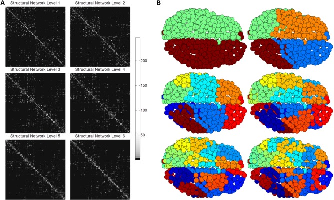
To illustrate PLACE‐based hierarchical modularity, Figure 1A shows the structural networks rearranged according to the community structure created from PLACE. Figure 1B visualizes, on the surface of an individual participant's brain, the subsequent extracted modular structure (each color represents one community) of the mean connectome, which is formed by averaging element‐wise the connectomes of all 39 subjects for the 620‐parcellation scheme (7 subjects out of 46 had disconnected networks and thus were excluded).

Measuring Modular Scale‐Dependence Information Transfer

To probe the proposed scale‐dependent information transfer across the entire brain connectome's modular hierarchy, we first define the following variable $\tau$ for any node i at any hierarchical level L:

$${\tau }_i^L=\frac{{\sum }_{j=1, 2,.,n }^{j\ne i}{(1/2)}^{\mathrm{L}\hspace{0.17em}-\hspace{0.17em}\text{min}\left(L, {\mathrm{L}\mathrm{e}\mathrm{v}\mathrm{e}\mathrm{l}}^{\mathrm{*}}\left(i,j\right)\right)}\mathrm{P}\mathrm{L}{(i,j)}^{‐1}}{{\sum }_{j=1, 2,.,n}^{j\ne i}{(1/2)}^{L\hspace{0.17em}-\hspace{0.17em}\min \left( L, {\mathrm{L}\mathrm{e}\mathrm{v}\mathrm{e}\mathrm{l}}^{\mathrm{*}}\left(i,j\right) \right)}}$$

Here n is the total number of ROIs, and Level*(i, j) indicates the most local hierarchy at which nodes i and j are still assigned to the same module (in PLACE community structures are extracted top‐down; thus we will use “low level” to indicate coarse or more global, and “high level” to indicate finer or more local with the root level which contains all nodes to be labeled level 0). Note that the above equation collapses to the standard nodal efficiency when computed at the root (L = 0):

$${\tau }_i^{L=0}=\frac{{\sum }_{j=1, 2,.,n}^{j\ne i}\mathrm{P}\mathrm{L}{(i,j)}^{‐1}}{n‐1}$$

Furthermore, the weighting term ${(1/2)}^{L\hspace{0.17em}‐\hspace{0.17em}min\left(L, {\mathrm{L}\mathrm{e}\mathrm{v}\mathrm{e}\mathrm{l}}^{*}\left(i,j\right)\right)}$ simply returns 1 if nodes i and j belong to the same module at level L, returns ½ if nodes i and j do not belong to the same module at level L, but do so at level L−1, ¼ if nodes i and j do not belong to the same module at level L or L−1, but do so at level L−2, and so forth. Thus, this factor gives more weights to the information exchange efficiency between nodes that remain in the same module at higher levels of hierarchy, and as a result $\tau$ can be interpreted as a hierarchically weighted nodal efficiency.

Next, as PLACE algorithm assigns nodes based on path lengths, plotting ${\tau }_i^L/{\tau }_i^0$ (y axis) against level of bifurcation (x axis) thus yields a monotonically increasing function, which then can be fitted with an exponential function ${\tau }_i^L/{\tau }_i^0=\mathrm{e}\mathrm{x}\mathrm{p}\left({\mu }_{i}L\right)$ where the rate constant ${\mu }_i$ is unique to each region. Intuitively, the rate constant ${\mu }_i$ thus represents the rate of decay in a given node's information exchange efficiency with other regions, as we move from fine‐to‐coarse or local‐to‐global along the modular hierarchy.

RESULTS

Hierarchical Modularity of the Structural Connectome

As predicted, PLACE algorithm successfully extracted hierarchical modular structures from the connectome of each of the subjects for all parcellation schemes (excluding those with disconnected networks. For visualization purposes, the hierarchical structure of the averaged connectome for the group, as a whole, is superimposed on one subject's brain. To illustrate PLACE‐based hierarchical modularity, Figure 1A shows the structural networks rearranged to match the community structure created from PLACE. The subsequent extracted modular structure (each color represents one community) of the averaged connectome is seen in Figure 1B, which is formed by averaging element‐wise the connectomes of all 39 subjects for the 620‐parcellation scheme (7 subjects out of 46 had disconnected networks and thus were excluded).

The Rate of Decay in Information Exchange

After the modular structures are extracted, for each ROI we then computed the vector ${(\tau }_i^0/{\tau }_i^0{, \tau }_i^1/{\tau }_i^0, {\tau }_i^2/{\tau }_i^0)$ and averaged them over all available subjects for that particular parcellation scheme. Figure 2 visualizes the group average ${\tau }_i^L/{\tau }_i^0=$ (y axis) versus the level (L) for all four schemes, showing, as we hypothesized, that $\frac{{\tau }_i^L}{{\tau }_i^0}$ is a monotonically increasing function with respect to L. For each node, ${\tau }_i^L/{\tau }_i^0$ against level of bifurcation is then fitted with an exponential function in the form: ${\tau }_i^L/{\tau }_i^0=\mathrm{e}\mathrm{x}\mathrm{p}\left({\mu }_{i}L\right)$.

Figure 2.

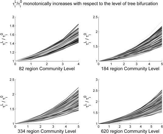
The proposed metric (y‐axis, ${\tau }_i^L/{\tau }_i^0$) in each ROI as we move from global (coarse) to local (fine) levels of modular hierarchy (x‐axis). As expected, the metric monotonically increases with respect to the level, indicating that a region has higher information transfer efficiencies with its closer neighbors. Here, each line represents a specific brain region's information transfer efficiency as the granularity increases.

Figure 3 visualizes this novel ${\mu }_i$ variable plotted against the standard nodal efficiency (i.e., ${\tau }_i^0$). Note that nodal efficiency ${\tau }_i^0$ decreases as the resolution or granularity of parcellation increases from 82 to 620, while the novel variable ${\mu }_i$ is relatively insensitive to parcellation resolution. Such observations are further confirmed by correlational analyses (Tables 1 and 2), which supported that μ values are highly correlated (thus relatively parcellation‐insensitive, also see Fig. 4) when compared across different parcellation schemes, as measured by both standard correlation coefficients and the ranking based on their values (Kendall's tau).

Figure 3.

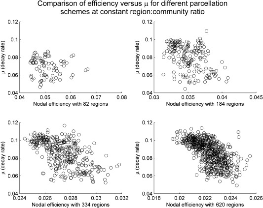
In this figure, we plot the rate constant μ, obtained from fitting ${\tau }_i^L/{\tau }_i^0=\mathrm{e}\mathrm{x}\mathrm{p}\left({\mu }_{i}L\right)$ for each region i, against the nodal efficiency in all four parcellation schemes. We note that in general less efficient nodes (those with low nodal efficiency ${\tau }_i^0$) tend to also have higher rates of decay; by contrast, nodes that have lower decay rate can have either low, medium, or high nodal efficiency ${\tau }_i^0$. In fact, if we restrict ourselves to nodes with decay rates ${\mu }_i$ less than 0.08, the correlation between ${\mu }_i$ and ${\tau }_i^0$ becomes statistically insignificant except for the 620‐parcelation scheme (P = 0.041) before correcting for multiple corrections (all insignificant after controlling for multiple comparisons).

Table 1.

This table shows the correlation coefficients for the nodal efficiency values between different parcellation schemes, and the Kendall's Tau correlations computed using the rank lists of these values

Correlation coefficients of efficiency between parcellation schemes
Values given are (correlation, Kendall's Tau)	Efficiency (82reg/8comm)	Efficiency (184reg/16comm)	Efficiency (334reg/32comm)	Efficiency (620reg/64comm)
Efficiency (82reg/8comm)	1.000,1.000	0.629,0.177	0.348,0.164	0.012,0.144
Efficiency (184reg/16comm)		1.000,1.000	0.808,0.153	0.510,0.011
Efficiency (334reg/32comm)			1.000,1.000	0.815,0.152
Efficiency (620reg/64comm)				1.000,1.000

Table 2.

This table shows the correlation coefficients for the μ values between different parcellation schemes, and the Kendall's Tau correlations computed using the rank lists of these values

Correlation coefficients of μ between parcellation schemes
Values given are (correlation, Kendall's Tau)	μ (82reg/8comm)	μ (184reg/16comm)	μ (334reg/32comm)	μ (620reg/64comm)
μ (82reg/8comm)	1.000,1.000	0.805,0.546	0.758,0.459	0.719,0.460
μ (184reg/16comm)		1.000,1.000	0.972,0.447	0.952,0.399
μ (334reg/32comm)			1.000,1.000	0.971,0.387
μ (620reg/64comm)				1.000,1.000

Comparing this table to Table 1, it is clear μ values are less dependent on the parcellation schemes than nodal efficiency.

Figure 4.

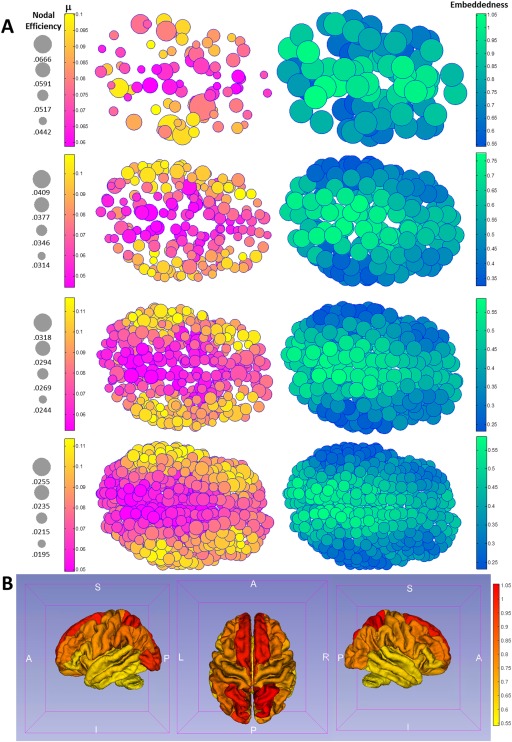
A visualizes both the decay rate constant ${\mu }_i$ (left panel) and the ratio ${\tau }_i^0/{\mathrm{\mu }}_i$ (right panel) neuroanatomically using top views for all four parcellation schemes on the brain surface of a representative subject. Note that visually trends are consistent across all schemes, showing both a posterior‐to‐anterior gradient and a medial‐to‐lateral gradient for ${\mu }_i$ and ${\tau }_i^0/{\mu }_i$ (the gradients are increasing for decay rate ${\mu }_i$ and decreasing for the ratio ${\tau }_i^0/{\mu }_i$). Figure 4B visualizes the embeddedness, as a heat map, on a Freesurfer‐defined group average cortical surface using the 82‐parcellation scheme.

Interestingly, we note that in general less efficient nodes (those with low nodal efficiency ${\tau }_i^0$) tend to also have higher rates of decay; by contrast, nodes that have lower decay rate can have either low, medium, or high nodal efficiency ${\tau }_i^0$. In fact, if we restrict ourselves to nodes with decay rates ${\mu }_i$ less than 0.08, the correlation between ${\mu }_i$ and ${\tau }_i^0$ becomes statistically nonsignificant after controlling for multiple comparisons (correlation coefficient r and P values for the 82, 184, 334, and 620 parcellation schemes were −0.134/0.274, −0.206/0.060, 0.180/0.054, and −0.144/0.041, respectively). These correlational results thus support that the decay rate constant μ captures scale‐dependent properties of the connectome that are not measured by single‐scale graph metrics such as standard nodal efficiency.

For the 82‐parcellation scheme, we additionally conducted post hoc multiple linear regression analyses to test an age effect (age measured in years) in the decay rate: ${\mu =\mu }^{\mathrm{i}\mathrm{n}\mathrm{t}\mathrm{e}\mathrm{r}\mathrm{c}\mathrm{e}\mathrm{p}\mathrm{t}}+{\mu }^{\mathrm{a}\mathrm{g}\mathrm{e}}\times \mathrm{a}\mathrm{g}\mathrm{e}$. Results revealed that both the left and right superior frontal gyrus exhibit an age effect (left superior frontal gyrus: μ ^age = −0.0013, P = 0.0021); right superior frontal gyrus μ ^age = −0.0012, P = 0.0054) before controlling for multiple comparisons (neither survived multiple comparison corrections using FDR).

Last, we propose to form the ratio ${\tau }_i^0/{\mathrm{\mu }}_i$, which can be thought of as a measure of hierarchical embeddedness of any brain region. By sorting this ratio from high to low one can highlight nodes that not only (1) have high nodal efficiency, but also (2) have slower decay from local to global across connectome's hierarchical modularity. Indeed, these regions not only communicate overall more efficiently with other brain regions, they do so across all levels of hierarchy (i.e., insensitive to scale changes).

Figure 4 visualizes both the decay rate constant ${\mu }_i$ and the “embeddedness” ratio ${\tau }_i^0/{\mathrm{\mu }}_i$ neuroanatomically using top views for all four parcellation schemes on the brain surface of a representative subject. Note that visually trends are consistent across all schemes, showing both a a medial‐to‐lateral gradient and (to a lesser degree) posterior‐to‐anterior gradient for ${\mu }_i$ and ${\tau }_i^0/{\mu }_i$ (the gradients are increasing for decay rate ${\mu }_i$ and decreasing for the ratio ${\tau }_i^0/{\mathrm{\mu }}_i$; the medial‐to‐lateral gradient is discussed in the Discussion Section, while the posterior‐to‐anterior gradient is possibly related to the rostro‐caudal gradient during neurodevelopment [Redies and Puelles, 2001]).

To better appreciate how the gradient of this ratio translates to known neuroanatomical regions, after averaging ${\mu }_i$ and ${\tau }_i^0$ within each of the original 82 Freesurfer anatomical labels using data from the 620‐parcellation scheme, Table 3 lists label‐averaged embeddedness ${\tau }_i^0/{\mathrm{\mu }}_i$ for the 82 anatomical regions, from high to low. Regions ranked higher here thus exhibit higher degrees of scale‐invariant efficiency in communicating with the rest of the network. Note that highly embedded brain regions are primarily the bilateral subcortical structures including the thalamus and basal ganglia, the regions forming the limbic system (insula, nucleus accumbens, and subdivisions of cingulum), the precuneus (part of the default mode network [Raichle et al., 2001]), superior parietal regions, and the medial orbitofrontal cortex. Figure 5 visualizes decay rate ${\mu }_i$ and embeddedness ${\tau }_i^0/{\mathrm{\mu }}_i$ for these regions using axial views (overlaid with high‐resolution T1‐weighted structural images from a representative subject; precuneus and neighboring parietal regions are best appreciated in slice A, basal ganglia, thalamus, and insula in slice B, and nucleus accumbens, medial temporal lobe and medial orbitofrontal cortex in slice C).

Table 3.

After averaging within each of the original 82 anatomical labels using data generated from the 620‐parcellation scheme, for both μ and nodal efficiency, the ratio of nodal efficiency to μ or “embeddedness” was computed and the regions were sorted and listed from high to low with respect to this ratio

Rank list of embeddedness for 82 freesurfer regions
Region Name	Embeddedness	Region Name	Embeddedness
ctx‐rh‐isthmuscingulate	0.389	ctx‐rh‐temporalpole	0.268
Right‐Pallidum	0.379	ctx‐rh‐parahippocampal	0.263
ctx‐rh‐posteriorcingulate	0.372	ctx‐lh‐lingual	0.262
Right‐Thalamus‐Proper	0.369	ctx‐lh‐pericalcarine	0.261
ctx‐lh‐isthmuscingulate	0.369	ctx‐lh‐entorhinal	0.26
ctx‐rh‐precuneus	0.361	ctx‐rh‐precentral	0.256
Left‐Pallidum	0.361	ctx‐lh‐precentral	0.254
Right‐Putamen	0.36	ctx‐rh‐pericalcarine	0.254
Left‐Putamen	0.357	ctx‐rh‐lateralorbitofrontal	0.251
Left‐Thalamus‐Proper	0.354	ctx‐rh‐lingual	0.251
ctx‐lh‐posteriorcingulate	0.35	ctx‐lh‐lateralorbitofrontal	0.25
ctx‐rh‐caudalanteriorcingulate	0.346	ctx‐rh‐entorhinal	0.248
ctx‐lh‐precuneus	0.343	ctx‐lh‐inferiorparietal	0.247
Left‐Accumbens‐area	0.332	ctx‐rh‐transversetemporal	0.245
Right‐Accumbens‐area	0.33	ctx‐rh‐parsorbitalis	0.245
ctx‐lh‐caudalanteriorcingulate	0.329	ctx‐rh‐superiortemporal	0.243
Right‐Caudate	0.328	ctx‐lh‐transversetemporal	0.243
ctx‐rh‐paracentral	0.328	ctx‐rh‐postcentral	0.243
ctx‐rh‐superiorparietal	0.326	ctx‐rh‐lateraloccipital	0.24
ctx‐lh‐paracentral	0.32	ctx‐lh‐superiortemporal	0.238
ctx‐lh‐insula	0.319	ctx‐rh‐parsopercularis	0.237
ctx‐lh‐superiorparietal	0.317	ctx‐lh‐caudalmiddlefrontal	0.236
Left‐Caudate	0.316	ctx‐lh‐parsopercularis	0.235
ctx‐lh‐medialorbitofrontal	0.307	ctx‐lh‐postcentral	0.233
ctx‐rh‐insula	0.305	ctx‐rh‐rostralmiddlefrontal	0.232
Right‐Amygdala	0.305	ctx‐lh‐parstriangularis	0.231
ctx‐rh‐medialorbitofrontal	0.3	ctx‐lh‐parsorbitalis	0.23
Left‐Amygdala	0.297	ctx‐rh‐parstriangularis	0.228
ctx‐rh‐frontalpole	0.297	ctx‐lh‐rostralmiddlefrontal	0.227
ctx‐rh‐rostralanteriorcingulate	0.293	ctx‐rh‐caudalmiddlefrontal	0.225
Left‐Hippocampus	0.291	ctx‐rh‐inferiorparietal	0.224
ctx‐lh‐cuneus	0.29	ctx‐lh‐fusiform	0.223
Right‐Hippocampus	0.288	ctx‐rh‐fusiform	0.221
ctx‐lh‐rostralanteriorcingulate	0.287	ctx‐lh‐inferiortemporal	0.22
ctx‐lh‐frontalpole	0.286	ctx‐rh‐middletemporal	0.217
ctx‐lh‐superiorfrontal	0.285	ctx‐rh‐bankssts	0.216
ctx‐rh‐superiorfrontal	0.282	ctx‐rh‐inferiortemporal	0.215
ctx‐lh‐lateraloccipital	0.276	ctx‐lh‐middletemporal	0.214
ctx‐lh‐parahippocampal	0.271	ctx‐rh‐supramarginal	0.209
ctx‐lh‐temporalpole	0.269	ctx‐lh‐bankssts	0.208
ctx‐rh‐cuneus	0.269	ctx‐lh‐supramarginal	0.199

Regions ranked higher thus not only (1) have high nodal efficiency, but also (2) have slower efficiency decay. Regions with the highest degrees of embeddedness are primarily the bilateral subcortical structures including the thalamus and basal ganglia (pallidum, caudate, and putamen), the regions forming the limbic system (insula, nucleus accumbens, and subdivisions of cingulum), the precuneus and neighboring parietal regions, and the medial orbitofrontal cortex.

Figure 5.

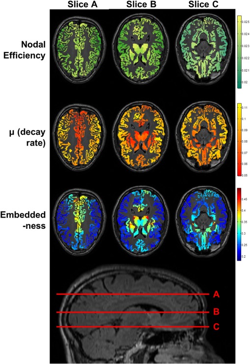
Shows regions with low decay rate ${\mu }_i$ and high ${\tau }_i^0/{\mu }_i$ ratio (embeddedness) using axial views overlaid with corresponding high‐resolution T1‐weighted structural images (top) from a representative subject with slices shown on a lateral view of the 3D brain (bottom). Here precuneus and neighboring parietal regions are best appreciated in slice A, basal ganglia, thalamus and insula in slice B, and nucleus accumbens, medial temporal lobe and medial orbitofrontal cortex in slice C. A sagittal slice for localization is shown at the bottom of the figure. Also see Table 3.

DISCUSSION

In this study, we proposed a multi‐scale approach to understand the property of “embeddedness” in structural brain connectome. The proposed approach is advantageous in that it collectively examines all levels of a connectome's hierarchical modularity, instead of restricting to one hierarchy in prior studies. To measure embeddedness, we quantified the rate of exponential decay in information exchange, from local to global or fine to coarse, across modular hierarchies. Post hoc analyses further revealed that this rate of decay exhibits no statistically significant age‐related changes across the whole brain. We then mathematically define “embeddedness” as the numerical inverse of this decay rate multiplied by nodal efficiency; nodes with high degrees of embeddedness thus not only communicate overall more efficiently with other brain regions, they do so with relative modular scale‐invariance.

To validate this multi‐scale approach, we investigated regional nodal embeddedness using diffusion weighted MR imaging data from a sample of 46 normal healthy human subjects. For all subjects, the structural connectome's hierarchical modularity was extracted using a path‐length based algorithm at four levels of parcel granularity: the original Freesurfer‐based parcellation as well as three upsampled schemes with mean parcel volumes of approximately 4, 2, and 1 cm³, respectively. Results supported that the rate of information exchange decay is relatively invariant with respect to the granularity of parcellation schemes. Moreover, while in general high decay rate is associated with low nodal efficiency, nodes with low decay rate displays wide‐ranging efficiency values (i.e., when restricted to lower values, decay rate dissociates from nodal efficiency), and thus they measure separate properties of the human brain connectome.

It is worth noting that although overall the decay rate μ remains relatively constant across adulthood with no evidence of a significant age‐dependence, there was however a trend toward a decreasing rate with age in the bilateral superior frontal gyrus before controlling for multiple comparisons. While age‐related changes in structure and function in select regions of the frontal lobe have been reported in the superior frontal gyrus [Convit et al., 2001; Solbakk et al., 2008; Wellington et al., 2013], the trend decrease in decay rate may additionally be consistent with the compensatory scaffolding (i.e., the recruitment of additional circuitry) theory in cognitive aging involving the frontal lobe [Park and Reuter‐Lorenz, 2009].

Computing group‐average nodal embeddedness and sorting them from high low, we showed that neuroanatomical regions with highest degrees of embeddedness are those comprising the limbic system, the subcortical nuclei (basal ganglia and thalamus), and the default mode network.

Our results have several implications. First, by successfully extracting hierarchical modularity we demonstrated that the human connectome, like many other types of complex systems in nature, exhibits the ubiquitous property of “near‐decomposability” as theorized in Simon [1965] which pioneered work on complex systems more than 50 years ago (in this theory, most complex systems are near‐decomposable systems, that is, there exists of a hierarchy of components, such that at any level of the hierarchy the rates of interaction within components are much higher than those between different components [Simon, 2002]). However, we additionally demonstrated that despite being nearly decomposable overall, select components of the human brain connectome further exhibit relative “embeddedness” (i.e., variability in the extent that a region's efficiency of communication persists through increasing distances of the network).

We note that the highly embedded brain regions detected in this study heavily (if not entirely) overlap with the recently proposed “revised limbic system” [Catani et al., 2013] model for memory, emotion and behavior. In this model, the authors updated the classic limbic model as proposed by Papez [1937] and Yakovlev et al. [1960] to include three distinct but partially overlapping networks: the Temporo‐amygdala‐orbitofrontal network, the Hippocampal‐diencephalic and parahippocampal‐retrosplenial network, and the Dorsomedial default network. Thus, our results offer connectome evidence for fundamental differences between the affective/limbic system and the executive/cognitive‐control system (the latter regions responsible for specialized and well‐defined higher cortical functions).

Our results may additionally support an evolutionarily value to a high degree of embedded integration of emotional information. Indeed, the limbic system has been a more ancient part of evolutionary development relative to higher level cognition. Therefore it makes sense that the former is better embedded from a system perspective; basic functions mediated by the limbic system require a diffuse pattern of integration and efficient access to the rest of the brain.

Note an analogy can thus be drawn between our findings and the “System 1/fast versus System 2/slow” conclusion discussed by Kahneman [2011] as part of a rapidly evolving new discipline—behavioral economics [Camerer et al., 2011; Colin and George, 2004] (here System 1 is the “brain's fast, automatic, intuitive approach while System 2 refers to the mind's slower analytical mode, where reason dominates” [Walsh, 2014]). Although both systems offer value in their respective ways, we posit that connectome conditions necessary for generating highly complex executive functions (highly localized and organized) are thus different from those necessary for generating intuition‐based functions (e.g., kneejerk reaction); to say it simply, one comes at the cost of the other.

The potential implication of our findings can be far‐reaching. For example, they further explain the well‐established emotional distractibility seen during cognitive tasks [Dolcos et al., 2014; Iordan et al., 2013]. Along these lines, a better understanding of various disease states might be understood. For instance, those with autism spectrum disorders might be viewed as having abnormalities in terms of the degree that emotional circuitry is embedded [Washington et al., 2014]. A difficulty in this area might explain why these individuals tend to gravitate toward activities with less emphasis on emotional integration. In this same light, those with savant skills might be viewed as not actually developing a new function, but rather that the loss of limbic embeddedness allows for unfettered functioning of brain regions built for highly complex mental operations.

To briefly compare our results with relevant findings in a recent study [Meunier et al., 2009] that similarly constructed hierarchical modularity using functional brain networks, we note that in that study the well‐known modularity metric (Q) was employed. Also, despite demonstrating modular hierarchies, the authors determined node roles based on the most global (nontrivial) modular decomposition, but qualitatively examined brain regions in each module at the most local level using one representative subject (instead of collectively investigating across all hierarchies as in this current study). Results also differ in their selection of modules in that they identify medial and lateral occipital areas amongst the largest modules. They note that occipital modules decompose towards a dominant sub‐module, whereas the other identified regions decompose more evenly into multiple sub‐modules. By contrast, our results indicated that occipital areas are relatively less embedded compared to the limbic system network, pointing to different utilities in the use of our method in assessing brain networks.

Another interesting concept to which we compare our results is the property of “rich‐club” organization in the human connectome [de Reus and van den Heuvel, 2014; Harriger et al., 2012; van den Heuvel and Sporns, 2011]. We note that similar to our medial‐to‐lateral gradient (Fig. 5), regions reported to be rich club (precuneus, superior frontal and superior parietal, as well as subcortical hippocampus, putamen and thalamus) are primarily medially located bi‐hemispherically. However, excluding the superior frontal cortex all rich‐club regions form a subset of the regions that we found to also exhibit higher degree of embeddedness. This suggests that the “rich‐clubness” and embeddedness are two distinct yet potentially complementary properties. Future studies are thus needed to further understand their relationship.

It should note that as a potential limitation of this study our data is derived from diffusion‐weighted MRI instead of functional MRI (fMRI). One may argue that the use of fMRI might elucidate variations in network architecture during various functional states (resting vs. task‐specific), as well as better understand the functional correlates of “embeddedness” as a novel network property. A future area of study would clearly be to apply the proposed technique to fMRI data. Other potential limitations may also include: (1) DTI as a method is based on numerous assumptions that may not reflect “actual” white matter pathways in the brain, this can lead to confounding results from anisotropic voxels, b‐value weighting, and tractography reconstruction algorithms; (2) PLACE's method of a bifurcating community structure may not be optimal in other studies of embeddedness, such as with functional MRI [Yeo et al., 2011]; (3) the concept of embeddedness needs to be replicated in larger datasets as well as using networks that arise in fields outside of neuroscience.

Last, the observed left‐right split for the first‐level bifurcation in our PLACE results may be related to the under‐estimation of inter‐hemispheric connections during DTI tractography, explaining the medial‐lateral gradient in the decay rate and embeddedness. We thus cross‐validated our approach using a second dataset (21 healthy subjects; mean age in years: 40.4 ± 10.1; 15 males) whose diffusion‐weighted MRI utilized a higher angular resolution (68 directions; 64 with a b value of 1,000 s/mm²; 4 b ₀ images) coupled with probabilistic tractography (see Supporting Information) [Behrens et al., 2007]. Interestingly, for this second dataset, PLACE varied its first‐level split between left/right and anterior/posterior, depending on the individual. However, all subjects had the complementary split happen in the following level (if the first level was an anterior/posterior split, the second level was a left/right split). The ordering of the first two levels could thus depend on individual differences during fiber reconstruction. Regardless, the correlations between the nodal efficiency, μ, and embeddedness values obtained from the two datasets were all statistically significant with P values less than 0.001, despite the fact that they were generated from two different samples using two different tractography reconstruction techniques.

CONCLUSION

This work presents a novel connectome approach to understand the property of embeddedness, that is, the degree of scale‐dependence of information exchange efficiency across levels of hierarchical modularity. Our results support that the structural human connectome exhibits: (1) overall near‐decomposability and (2) selective embeddedness in brain regions within the “limbic network” (including the limbic system, subcortical structures, and regions known to be part of the default mode network). That is, these regions display higher degrees of information exchange efficiency with lower decay. Results may have clinical implication, in that such topological differences may provide structural evidence of the prioritization of limbic network‐mediated information, possibly in the context of its enhanced evolutionary value.

Supporting information

Supporting Information

REFERENCES

- Ajilore O, Zhan L, GadElkarim J, Zhang A, Feusner JD, Yang S, Thompson PM, Kumar A, Leow A (2013): Constructing the resting state structural connectome. Front Neuroinform 7:1–8. [DOI] [PMC free article] [PubMed] [Google Scholar]
- Behrens T, Berg HJ, Jbabdi S, Rushworth M, Woolrich M (2007): Probabilistic diffusion tractography with multiple fibre orientations: What can we gain?. Neuroimage 34:144–155. [DOI] [PMC free article] [PubMed] [Google Scholar]
- Blondel VD, Guillaume J‐L, Lambiotte R, Lefebvre E (2008. ): Fast unfolding of communities in large networks. J Stat Mech Theory Exp 2008:P10008. [Google Scholar]
- Camerer CF, Loewenstein G, Rabin M (2011): Advances in Behavioral Economics Princeton, New Jersey, USA. [Google Scholar]
- Cao Q, Shu N, An L, Wang P, Sun L, Xia M‐R, Wang J‐H, Gong G‐L, Zang Y‐F, Wang Y‐F, He Y (2013): Probabilistic diffusion tractography and graph theory analysis reveal abnormal white matter structural connectivity networks in drug‐naive boys with attention deficit/hyperactivity disorder. J Neurosci 33:10676–10687. [DOI] [PMC free article] [PubMed] [Google Scholar]
- Catani M, Dell'Acqua F, Thiebaut de Schotten M (2013): A revised limbic system model for memory, emotion and behaviour. Neurosci Biobehav Rev 37:1724–1737. [DOI] [PubMed] [Google Scholar]
- Colin C, George L (2004): Behavioral Economics: Past, Present, Future Princeton: Princeton University Press. [Google Scholar]
- Colizza V, Flammini A, Serrano MA, Vespignani A (2006): Detecting rich‐club ordering in complex networks. Nat Phys 2:110–115. [Google Scholar]
- Convit A, Wolf OT, de Leon MJ, Patalinjug M, Kandil E, Caraos C, Scherer A, Saint Louis LA, Cancro R (2001): Volumetric analysis of the pre‐frontal regions: Findings in aging and schizophrenia. Psychiatry Res Neuroimaging 107:61–73. [DOI] [PubMed] [Google Scholar]
- De Reus MA, van den Heuvel MP (2014): Simulated rich club lesioning in brain networks: A scaffold for communication and integration?. Front Hum Neurosci 8:1–5. [DOI] [PMC free article] [PubMed] [Google Scholar]
- Dijkstra EW (1959): A note on two problems in connexion with graphs. Numer Math 1:269–271. [Google Scholar]
- Dolcos F, Wang L, Mather M (2014): Current research and emerging directions in emotion‐cognition interactions. Front Integr Neurosci 8:1–11. [DOI] [PMC free article] [PubMed] [Google Scholar]
- Fisher FM (1961): On the cost of approximate specification in simultaneous equation estimation. Econometrica 29:139–170. [Google Scholar]
- GadElkarim JJ, Schonfeld D, Ajilore O, Zhan L, Zhang AF, Feusner JD, Thompson PM, Simon TJ, Kumar A, Leow AD (2012): A framework for quantifying node‐level community structure group differences in brain connectivity networks. Med Image Comput Comput Assist Interv 15:196–203. [DOI] [PMC free article] [PubMed] [Google Scholar]
- GadElkarim JJ, Ajilore O, Schonfeld D, Zhan L, Thompson PM, Feusner JD, Kumar A, Altshuler LL, Leow AD (2014): Investigating brain community structure abnormalities in bipolar disorder using path length associated community estimation. Hum Brain Mapp 35:2253–2264. [DOI] [PMC free article] [PubMed] [Google Scholar]
- Guimera R, Amaral LAN (2005): Cartography of complex networks: Modules and universal roles. J Stat Mech Theory Exp 2005:P02001. [DOI] [PMC free article] [PubMed] [Google Scholar]
- Harriger L, van den Heuvel MP, Sporns O (2012): Rich club organization of macaque cerebral cortex and its role in network communication. PLoS ONE 7:e46497. [DOI] [PMC free article] [PubMed] [Google Scholar]
- Iordan AD, Dolcos S, Dolcos F (2013): Neural signatures of the response to emotional distraction: A review of evidence from brain imaging investigations. Front Hum Neurosci 7:1–21. [DOI] [PMC free article] [PubMed] [Google Scholar]
- Kahneman D (2011): Thinking, fast and slow. Macmillan, London, United Kingdom.
- Meunier D, Lambiotte R, Fornito A, Ersche KD, Bullmore ET (2009): Hierarchical modularity in human brain functional networks. Front Neuroinform 3:1–12. [DOI] [PMC free article] [PubMed] [Google Scholar]
- Mori S, Crain BJ, Chacko VP, Van Zijl PCM (1999): Three‐dimensional tracking of axonal projections in the brain by magnetic resonance imaging. Ann Neurol 45:265–269. [DOI] [PubMed] [Google Scholar]
- Newman M, Girvan M (2004): Finding and evaluating community structure in networks. Phys Rev E 69:1–15. [DOI] [PubMed] [Google Scholar]
- Papez JW (1937): A proposed mechanism of emotion. Arch Neurol Psychiatry 38:725–743. [Google Scholar]
- Park DC, Reuter‐Lorenz P (2009): The adaptive brain: Aging and neurocognitive scaffolding. Annu Rev Psychol 60:173. [DOI] [PMC free article] [PubMed] [Google Scholar]
- Raichle ME, MacLeod AM, Snyder AZ, Powers WJ, Gusnard DA, Shulman GL (2001): A default mode of brain function. Proc Natl Acad Sci U S A 98:676–682. [DOI] [PMC free article] [PubMed] [Google Scholar]
- Redies C, Puelles L (2001): Modularity in vertebrate brain development and evolution. BioEssays 23:1100–1111. [DOI] [PubMed] [Google Scholar]
- Simon HA (1965): The architecture of complexity. Gen Syst 10:63–76. [Google Scholar]
- Simon HA (2002): Near decomposability and the speed of evolution. Ind Corp Change 11:587–599. [Google Scholar]
- Simon HA, Ando A (1961): Aggregation of variables in dynamic systems. Econometrica 29:111–138. [Google Scholar]
- Solbakk A‐K, Alpert GF, Furst AJ, Hale LA, Oga T, Chetty S, Pickard N, Knight RT (2008): Altered prefrontal function with aging: Insights into age‐associated performance decline. Brain Res 1232:30–47. [DOI] [PMC free article] [PubMed] [Google Scholar]
- Sporns O, Tononi G, Kötter R (2005): The human connectome: A structural description of the human brain. PLoS Comput Biol 1:e42. [DOI] [PMC free article] [PubMed] [Google Scholar]
- Sporns O, Honey CJ, Kötter R (2007): Identification and classification of hubs in brain networks. PloS One 2:e1049. [DOI] [PMC free article] [PubMed] [Google Scholar]
- Sun L, Cao Q, Long X, Sui M, Cao X, Zhu C, Zuo X, An L, Song Y, Zang Y, Wang Y (2012): Abnormal functional connectivity between the anterior cingulate and the default mode network in drug‐naïve boys with attention deficit hyperactivity disorder. Psychiatry Res Neuroimaging 201:120–127. [DOI] [PubMed] [Google Scholar]
- Van den Heuvel MP, Sporns O (2011): Rich‐club organization of the human connectome. J Neurosci 31:15775–15786. [DOI] [PMC free article] [PubMed] [Google Scholar]
- Walsh C (2014): Layers of choice. Harvard Gazette, February 5. Available at http://news.harvard.edu/gazette/story/2014/02/layers-of-choice/#pq=v10mwP. Last Accessed, February 7, 2015.
- Washington SD, Gordon EM, Brar J, Warburton S, Sawyer AT, Wolfe A, Mease‐Ference ER, Girton L, Hailu A, Mbwana J, Gaillard WD, Kalbfleisch ML, VanMeter JW (2014): Dysmaturation of the default mode network in autism. Hum Brain Mapp 35:1284–1296. [DOI] [PMC free article] [PubMed] [Google Scholar]
- Wellington RL, Bilder RM, Napolitano B, Szeszko PR (2013): Effects of age on prefrontal subregions and hippocampal volumes in young and middle‐aged healthy humans. Hum Brain Mapp 34:2129–2140. [DOI] [PMC free article] [PubMed] [Google Scholar]
- Yakovlev P, Locke S, Koskoff D, Patton R (1960): Limbic nuclei of thalamus and connections of limbic cortex. Arch Neurol 3:620–641. [DOI] [PubMed] [Google Scholar]
- Yeo BTT, Krienen FM Sepulcre J, Sabuncu MR, Lashkari D, Hollinshead M, Roffman JL, Smoller JW, Zollei L, Polimeni JR, Fischl B, Liu H, Buckner RL (2011): The organization of the human cerebral cortex estimated by intrinsic functional connectivity. J Neurophysiol 106:1125–1165. [DOI] [PMC free article] [PubMed] [Google Scholar]
Associated Data
This section collects any data citations, data availability statements, or supplementary materials included in this article.
Supplementary Materials