Nonparametric survival analysis using Bayesian Additive Regression Trees (BART)

Abstract

Bayesian additive regression trees (BART) provide a framework for flexible nonparametric modeling of relationships of covariates to outcomes. Recently, BART models have been shown to provide excellent predictive performance, for both continuous and binary outcomes, and exceeding that of its competitors. Software is also readily available for such outcomes. In this article we introduce modeling that extends the usefulness of BART in medical applications by addressing needs arising in survival analysis. Simulation studies of one-sample and two-sample scenarios, in comparison with long-standing traditional methods, establish face validity of the new approach. We then demonstrate the model’s ability to accommodate data from complex regression models with a simulation study of a nonproportional hazards scenario with crossing survival functions, and survival function estimation in a scenario where hazards are multiplicatively modified by a highly nonlinear function of the covariates. Using data from a recently published study of patients undergoing hematopoietic stem cell transplantation, we illustrate the use and some advantages of the proposed method in medical investigations.

1. Introduction

Survival analysis addresses data that contain information on the time to occurrence of some event, often death or relapse after treatment for a disease. A common feature of such time-to-event data is right-censoring, caused by some observations for which the event time is not available but it is known that the event did not occur until some observed time point. The literature contains a rich set of models and analysis methods for such data in a wide variety of contexts [1, 2, 3, 4, 5]. Survival analysis naturally focuses on the probability S(t) that the event does not occur by time t for all t > 0. Also of interest is the hazard h(t), the time rate of the probability of event occurrence in the next instance given that it has not occurred by time t. These functions and various aspects of them are targets of inference when data are available from a homogeneous population [6, 7, 8, 9, 10]. Comparison of these functions is the focus when two or more populations arise as, for example, in considering alternative treatments for a disease [11, 12, 13].

More generally, in a regression context, investigators quantify how these inference targets vary with the values of a regressor x. The Cox proportional hazards model [14, 15, 16] is a popular choice for regression. It has also been well scrutinized [17, 18, 19] and alternatives have been proposed [20, 21, 22]. In practice, regression relationships in survival data are often complex. These can include nonlinear functions of covariates, interactions, high dimensional parameter spaces and nonproportional hazards. Several solutions have been proposed; for example, using lasso-type penalization [23, 24, 25], boosting with Cox-gradient descent [26, 27] and random survival forests [28]. We describe in this paper new methodology that can be readily used for many of these contexts. While we demonstrate its usefulness and advantages only in some focused contexts here, we believe it can be adapted to most of those mentioned in this and the previous paragraph.

Single tree based methods developed in the 1980’s and 90’s [29, 30, 31] have been extended more recently to ensemble methods that use a sizable set of trees [32, 33, 34]. These models perform very well for their originally intended purpose: fitting nonlinear functional relationships in regression. A particularly successful development, one that also includes measures of uncertainty in the resulting predictions, is the BART (Bayesian Additive Regression Trees) model [35]. The authors of the article demonstrate, via simulations in a variety of scenarios, that BART compares favorably with its competitors such as boosting, lasso, MARS, neural nets and random forests. We employ BART in this paper because of its predictive performance and its natural quantification of uncertainty that allows construction of credible and prediction intervals. Like its competitors, BART can effectively address nonlinear relationships of a response variable to a (possibly large) set of regressors. As these relationships are estimated simultaneously with all the regressors, possible interactions between them are automatically addressed by tree based methods. In addition, it has been demonstrated that BART’s excellent predictive performance is maintained when additional irrelevant regressors are added [35](page 288), diminishing the need to carry out variable or model selection. However, it is also possible to carry out variable selection [35](page 276) and quantitatively describe the effect of individual variables on the outcome.

Recently, BART methodology has been employed by Bonato et al. [36] for survival prediction. They present three specific models – proportional hazards regression, Weibull regression and accelerated failure time (AFT) – where the tree ensembles are used primarily on the covariate structure in hierarchical specifications. In the first, the baseline survival distribution is modeled separately via a Gamma process. The second uses a parametric baseline form with the log of the scale parameter incorporated into the tree ensemble. The third, being an AFT model, addresses survival times on the log scale treated as normally distributed variates. We propose here a more direct, simpler and widely applicable adaptation of BART that relaxes the parametric and semiparametric assumptions in [36]. This is made possible by expressing the nonparametric likelihood for the Kaplan-Meier estimator in a form suitable for BART. The resulting method not only uses the stochastic framework of BART but also allows one to employ existing BART software by suitably rearranging data constructed for traditional (frequentist or Bayesian) survival analysis.

We present our work in the following sequence. In Section 2 we describe BART methodology briefly, and then show its direct adaptation to survival analysis. Section 3 studies the performance of the proposed methods, first demonstrating the face validity of the proposed method in the simplest scenario of estimating the survival function for a homogeneous population. We do this by comparison with the Kaplan-Meier estimator. Next we extend this to a comparison of two populations. In Section 4 we demonstrate the model’s ability to accommodate data from complex regression models, and we provide a medical application that illustrates the advantages of the proposed methodology. A discussion in Section 5, of our contribution as well as of some planned future developments, concludes the article.

2. BART methodology for survival analysis

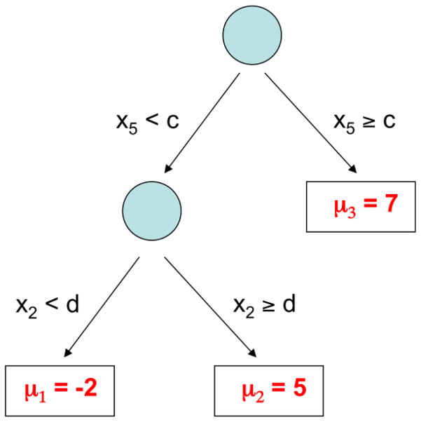
As BART is based on a collection of regression tree models, we begin with a simple example of a regression tree model. Suppose y_i represents an outcome, and x_i is a vector of covariates with the regression relationship y_i = g(x_i; T, M) + ε_i. Notationally, g(x_i; T, M) is a binary tree function with components T and M that can be described as follows. T denotes the tree structure consisting of two sets of nodes, interior and terminal, and a branch decision rule at each interior node which typically is a binary split based on a single component of the covariate vector. An example is shown in Figure 1 wherein interior nodes appear as circles, and terminal nodes as rectangles. The second tree component M = {μ₁,..., μ_b} is made up of the function values at the terminal nodes.

Figure 1.

An example of a single tree with branch decision rules and terminal nodes

BART employs an ensemble of such trees in an additive fashion, i.e., it is the sum of m trees where m is typically large such as 200, 500 or 1000. The model can be represented as:

$$\begin{array}{lll}\hfill y_i& =\hfill & f({\mathit{x}}_i)+{\epsilon }_i\text{where}{\epsilon }_i\stackrel{\text{iid}}{\sim }\mathrm{N}\left(0,{\sigma }^2\right)\hfill \\ \hfill f({\mathit{x}}_i)& =\hfill & {\sum }_{j=1}^{m}g({\mathit{x}}_i;T_j,M_j)\hfill \end{array}\}.$$ (1)

To proceed with the Bayesian specification we need a prior for f. Notationally, we use

$$f~\text{BART}$$ (2)

and describe it as made up of two components: a prior on the complexity of each tree, T_j, and a prior on its terminal nodes, M_j|T_j. Using the Smith-Gelfand bracket notation [37] for distributions, we write [f] = Π_j [T_j][M_j|T_j]. Following [35], we partition [T_j] into 3 components: the probability of a node being interior, the choice of a covariate given an interior node and the choice of decision rule given a covariate for an interior node. The probability that a node at depth d is interior is defined to be α(1 + d)^−γ where α ∈ (0, 1) and γ ≥ 0. We assume that the choice of a covariate given an interior node and the choice of decision rule branching value given a covariate for an interior node are both uniform. Throughout this article we have employed the default prior settings as described in [35], i.e., α = 0.95 and γ = 2. This choice of γ is a relatively large value reflecting a belief that the depth of the tree should be small, i.e., the probability decays rapidly with increasing d as can be seen in Table 1. We then use the prior $\left[M_j\mid T_j\right]={\prod }_{k=1}^{b_j}\left[{\mu }_{jk}\right]$ where μ_jk ~ N (0, 2.25/m) on the values of the terminal nodes. Along with centering of the outcome, these default prior mean and variance are specified such that each tree is a “weak learner” playing only a small part in the ensemble; more details on this can be found in [35]. To complete the Bayesian model in Equations (1) and (2), in general, we need a prior on σ². However, as we next describe, a reformulation of the model for survival data uses a probit regression with latent variables that have unit variance. For our purposes then, σ² = 1.

Table 1.

Tree complexity given default prior settings: α = 0.95 and γ = 2

Number of terminal nodes, b	1	2	3	4	5+
Prior probability	0.05	0.55	0.28	0.09	0.03

There are many potential approaches that could be taken to utilize BART in survival analysis. We describe a simple and direct approach that is very flexible, and is akin to discrete-time survival analysis [38]. Following the capabilities of BART, we allow for maximum flexibility in modeling the dependence of survival times on covariates. In particular, we do not impose proportional hazards. To elaborate, consider data in the usual form: t_i, δ_i, x_i where t_i is the event time, δ_i is an indicator distinguishing events (δ = 1) from right-censoring (δ = 0), x_i is a vector of covariates, and i = 1,..., n indexes subjects. We denote the k distinct event and censoring times by 0 < t₍₁₎ < · · · < t_(k) < ∞ thus taking t_(j) to be the j^th order statistic among distinct observation times and, for convenience, t₍₀₎ = 0. Now consider event indicators y_ij for each subject i at each distinct time t_(j) up to and including the subject’s observation time t_i = t_(ni) with n_i = #{j : t_(j) ≤ t_i}. This means y_ij = 0 if j < n_i and y_ini = δ_i. We then denote by p_ij the probability of an event at time t_(j) conditional on no previous event. We now write the model for y_ij as a nonparametric probit regression of y_ij on the time t_(j) and the covariates x_i, and then utilize the Albert-Chib [39] truncated normal latent variables z_ij to reduce it to the continuous outcome BART model of Equations (1–2) applied to z’s. Specifically, with data converted from (t, δ) pairs to

$$y_{ij}={\delta }_i\mathrm{I}\left(t_i=t_{(j)}\right),j=1,\dots ,n_i$$ (3)

we have

$$\begin{array}{lll}\hfill y_{ii}\mid p_{ij}& ~\hfill & \mathit{Bernoulli}(p_{ij})\hfill \\ \hfill p_{ij}\mid f& =\hfill & \mathrm{\Phi }({\mu }_{ij}),{\mu }_{ij}={\mu }_0+f(t_{(j)},x_i)\hfill \\ \hfill f& ~\hfill & \text{BART}\hfill \\ \hfill z_{ij}\mid y_{ij},f& ~\hfill & \{\begin{array}{ll}\mathrm{N}\left({\mu }_{ij},1\right)\mathrm{I}(-\infty ,0)\hfill & \text{if}{y}_{ij}=0\hfill \\ \mathrm{N}\left({\mu }_{ij},1\right)\mathrm{I}(0,\infty )\hfill & \text{if}{y}_{ij}=1\hfill \end{array}\hfill \end{array}\}.$$ (4)

This model in display (4) views the data vector y as made up of n independent sequences of 0’s and 1’s given p (the entire collection of p_ij’s). Consequently, we have the distribution

$$[\mathit{y}\mid \mathit{p}]=\prod _{i=1}^n\prod _{j=1}^{n_i}{p}_{ij}^{y_{ij}}{(1-p_{ij})}^{1-y_{ij}}.$$ (5)

We note here that the product over j is a result of the definition of p_ij’s as conditional probabilities, and not a consequence of an assumption of independence.

Remark on choice of μ₀: For the continuous outcome model of Equations (1–2), typically the outcome is centered and μ₀ is taken to be 0. In most cases with moderate or larger sample size centering, while helpful in computation, is not necessary because of the flexibility of f. For binary data, μ₀ = Φ⁻¹(p̂) can be used for centering the latent z’s. For the examples and simulations in this article, comparisons of results with and without centering found no meaningful differences. Reported results in Sections 4.1 and 4.2 are with centering, all others without.

The model just described can be readily estimated using existing software for binary BART. It allows one to estimate the functions f(t, x) or p(t, x) = Φ(μ₀ + f(t, x)). We now need to relate these back to the objectives of survival analysis. The next subsections address this issue, and give a simple example of data construction for use in binary BART.

2.1. Data construction

Survival data contained in pairs (t, δ) must be translated to data suitable for the BART model in Display (4). While the description of this is contained in Equation (3) and the definitions preceding it, for additional clarification we give here a very simple example of a data set with three observations:

$$(t_1,{\delta }_1)=(2.5,1),(t_2,{\delta }_2)=(1.5,1),(t_3,{\delta }_3)=(3.0,0)\text{with}{t}_{(1)}=1.5,t_{(2)}=2.5,t_{(3)}=\mathrm{3.0.}$$

In the t and y vectors, t₁ = 2.5 generates n₁ = 2 elements each since it is the 2^nd order statistic among distinct observation times. These elements are (t₁₁, t₁₂) = (1.5, 2.5), corresponding to distinct times up to and including t₁ = 2.5, and (y₁₁, y₁₂) = (0, 1) indicating the event status of this subject at each of these times. Similarly, t₂ = 1.5 generates n₂ = 1 element each: (t₂₁) = (1.5), (y₂₁) = (1); and t₃ = 3.0 generates n₃ = 3 elements (t₃₁, t₃₂, t₃₃) = (1.5, 2.5, 3.0) and (y₃₁, y₃₂, y₃₃) = (0, 0, 0). Putting these together leads to

$$\begin{array}{lll}\hfill {\mathit{y}}^{\prime }& =\hfill & (y_{11},y_{12},y_{21},y_{31},y_{32},y_{33})=(0,1,1,0,0,0)\hfill \\ \hfill {\mathit{t}}^{\prime }& =\hfill & (t_{11},t_{12},t_{21},t_{31},t_{32},t_{33})=(1.5,2.5,1.5,1.5,2.5,3.0)\hfill \end{array}$$

where y is the binary response vector and t makes up the first column of the matrix of covariates. The remaining columns contain the individual level covariates with rows repeated to match the repetition pattern of the first subscript on y.

2.2. Targets for inference

With the data prepared as described above, the BART model for binary data treats the conditional probability of the event in an interval, given no events in preceding intervals, as a nonparametric function of the time t and the covariates x. Conditioned on the data, the algorithm in the available software [40] generates samples, each containing m trees, from the posterior distribution of f. For any t and x then, we can obtain the posterior distribution of

$$p(t,\mathit{x})=\mathrm{\Phi }({\mu }_0+f(t,\mathit{x})).$$

For the purposes of survival analysis, we are typically interested in estimating the survival and hazard functions. Noting the discretized likelihood in equation (5) and the conditional nature of the probabilities p_ij, we write the following expressions to compute these functions at event/censoring times t_(j), j = 1,..., k:

$$\begin{array}{c}S(t_{(j)}\mid \mathit{x})=Pr(T>t_{(j)}\mid \mathit{x})=\prod _{l=1}^j(1-p(t_{(l)},\mathit{x}))\\ h(t_{(j)}\mid \mathit{x})=\frac{p(t_{(j)},\mathit{x})}{(t_{(j)}-t_{(j-1)})}.\end{array}$$

With these functions in hand, one can easily accomplish inference for other quantities of interest such as median or other percentiles of time to event, comparative hazards at various time points, etc.

Remark

The above expressions for hazard and survival functions are applicable only at the distinct observation times. Interpolation between these times can be accomplished via the usual assumption of constant hazard. In particular, h(t|x) = h(t_(j)|x) for all t ∈ (t_(j−1), t_(j)] and

$$S(t\mid \mathit{x})=\left(1-\frac{(t-t_{(j-1)})}{(t_{(j)}-t_{(j-1)})}p(t_{(j)},\mathit{x})\right)\prod _{l=0}^{j-1}(1-p(t_{(l)},\mathit{x})).$$

2.3. Marginal Effects

The model in Display (4) does not directly provide a summary of the effect of a single covariate or a subset of covariates. In general, this is true in the case of nonparametric regression models, in contrast to semi-parametric models. See, for example, the ANOVA dependent Dirichlet process model in [22]. Here we follow [35] and use Friedman’s partial dependence function [33] to summarize the marginal effect due to the covariates of interest by averaging over the others. To be explicit, partition the covariates as ${\mathit{x}}^{\prime }=({\mathit{x}}_I^{\prime },{\mathit{x}}_O^{\prime })$. Then the marginal dependence function is defined as

$$f({\mathit{x}}_I)=\frac{1}{n}\sum _{i=1}^{n}f({\mathit{x}}_I,{\mathit{x}}_{iO}).$$

This leads to

$$S(t\mid {\mathit{x}}_I)=\frac{1}{n}\sum _{i=1}^{n}S(t\mid {\mathit{x}}_I,{\mathit{x}}_{iO}).$$ (6)

Other marginal functions can be obtained in a similar fashion. Estimates then can be taken as means or medians over the samples from the posterior.

3. Performance of proposed methods: one and two samples

In this section we study, via repeated-data simulations, the performance of the BART survival model of display (4). The one-sample scenario is considered mainly to establish the face validity of the method by comparison with the long established Kaplan-Meier (KM) estimate of the survival function. Next the two-sample scenario is considered by fitting a single BART model and comparing it to a difference of two separate KM estimates.

3.1. One-sample scenario

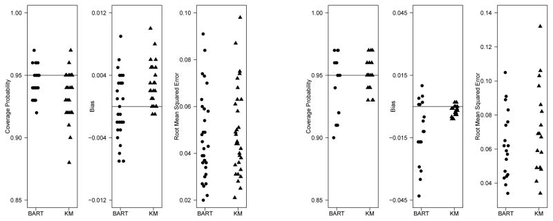
We generated event times from a Weibull survival curve, S(t) = e^−(t/λ)α, with parameters α = 0.8 and λ = 2.5. Censoring times were generated independently from an exponential distribution with parameters selected to induce 20% or 50% censoring. We examined sample sizes of N = 50, 100, and 200. For each simulation scenario, 400 data sets were generated. For each data set, the survival curve was estimated using the mean of the BART posterior distribution of the survival curve at 10^th,25^th, 50^th, 75^th and 90^th percentiles of the true distribution, leading to 30 simulation scenarios. In addition, 95% posterior intervals were obtained from the 0.025 and 0.975 quantiles of the posterior survival distribution. For comparison, we also obtained estimates and 95% confidence intervals based on the Kaplan-Meier estimate (using log transformation for the confidence intervals). For each sample size and censoring percentage, we summarized the results in terms of coverage probability, bias, and root mean squared error at the 5 selected percentiles of the survival distribution. These results are summarized in the left panel of Figure 2. Detailed comparisons by sample sizes, censoring percentages and the selected percentiles are included in the Supplement. In general, the posterior intervals from the BART model have very good coverage probabilities, comparable to the usual KM estimates. The bias of the BART model estimate is close to 0 across all the time points and comparable to but somewhat larger than that of the KM estimate. Finally, the BART model’s root mean square error across all included time points is comparable to but slightly smaller than that of the KM estimate. Overall, the BART model formulation is very effective in fitting a survival function.

Figure 2.

Dot plots of coverage probability, bias and root mean squared error for all 30 simulation settings for one-sample (left panel) and two-sample (right panel) studies. Each dot constructed from 400 simulated data sets.

3.2. Two-sample scenario

Next we studied the ability of the BART model to accurately fit two survival curves for two different populations in a single regression model. A group indicator x_i, i = 1,..., N for individual i was independently generated from a Bernoulli distribution with probability 0.5. Based on this indicator, event times were generated from one of two Weibull distributions, with α = 0.8, λ = 2.5 when x = 0 and α = 1.3, λ = 3.55 when x = 1. We selected these parameters to obtain crossing survival curves for the two populations. Such a scenario is typically more difficult to estimate in a single regression model. As in the one-sample simulation, independent exponential censoring times were generated with parameters chosen to induce either 20% or 50% censoring proportions overall. Total sample sizes of N = 100, 200, and 400 were studied. For each scenario, 400 data sets were simulated. We focused on the difference in survival between these two groups, S (t |x = 1) - S (t |x = 0), evaluated at the quartiles of the overall survival distribution. We compared the BART model, which fits a single nonparametric regression model to the data, with an analysis using the difference in Kaplan-Meier estimates between the two groups. Again, we evaluated the performance of each strategy in terms of coverage probability, bias, and root mean squared error. The results are shown in the right panel of Figure 2. Detailed tables are included in the Supplement.

In general, the posterior intervals from the BART model have good coverage probabilities which are comparable to that of the difference in KM estimates. Bias from both methods is low, although in some cases the BART model tends to have higher bias compared to the difference in KM estimates. Despite the higher bias of the BART method, its root MSE is comparable to and usually lower than that of the difference in KM estimates. This is likely because BART borrows some information across the two samples, reducing the variability of the estimates.

4. Regression

While the BART method compares quite favorably with KM in the one and two sample cases, its usefulness in practice lies in more complex regression scenarios. Survival analysis literature offers many different semiparametric models for regression such as Cox proportional hazards, proportional odds, accelerated failure times, additive hazards etc. Each of these relies on a particular functional relationship of the covariates to some aspect of the survival distribution. BART offers a flexible approach allowing nonparametric functional relationships. In this section we demonstrate such ability of this method via two simulation studies, and in a medical study.

4.1. Performance in regression scenarios, with and without proportional hazards

We designed two simulation settings, one following the commonly used Cox proportional hazards model (PH) and another (nPH) that would pose significant challenges, especially to traditional methods. We considered 9 independent binary covariates, x = [x₁,...,x₉]′, each with Bernoulli probability of 0.5, which then were related to the Weibull event time t with survival function S (t|α, λ) = e^−(t/λ)α through the rate/scale parameter alone (PH) and through both parameters (nPH) as follows:

$$\begin{array}{c}\text{PH}:\alpha =2.0,\lambda =\mathit{exp}\{3+0.1(x_1+x_2+x_3+x_4+x_5+x_6)+x_7\}\\ \text{nPH}:\alpha =0.7+1.3x_7,\lambda =20+5(x_1+x_2+x_3+x_4+x_5+x_6+10x_7)\end{array}$$

Note that x₈ and x₉ were excluded from outcome generation but retained in the covariates used in model estimation.

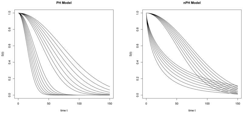
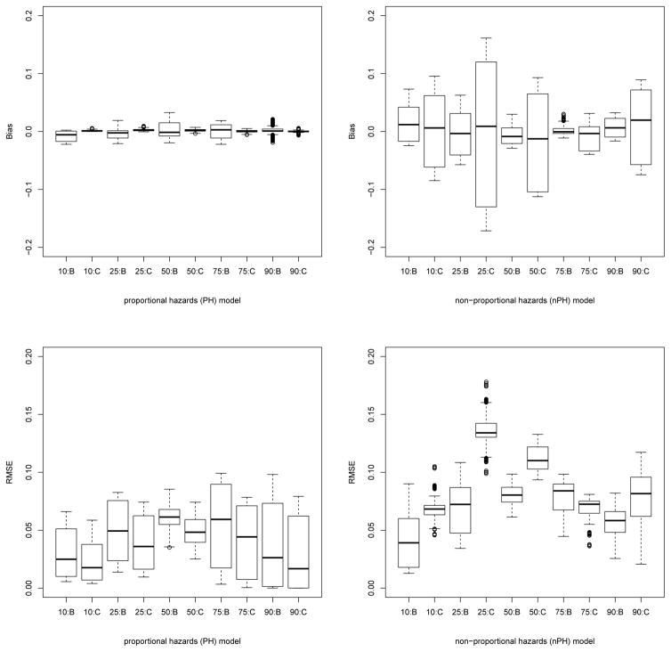
There are 2⁹ = 512 potential covariate configurations not all of which will be observed in any given data set, and these covariate configurations result in 14 distinct survival curves, as shown in Figure 3. We generated data sets of size N = 400, and used independent exponential censoring as before, yielding an overall censoring percentage of 20%. For each model, we generated 400 data sets and used them to evaluate bias for prediction of survival under each of the 512 potential covariate configurations. Using the survival R package, on each data set we also carried out Cox regression analysis with the covariates. Figure 4 shows box plots of bias and root mean squared error (RMSE) for the 512 configurations, measured at the 10^th,25^th,50^th,75^th and 90^th percentiles of the overall survival distribution. In the PH model, as expected, Cox regression analysis performs very well with respect to bias as well as RMSE. It is worth noting that the BART method is reasonably close to this in its performance. On the other hand, in the nPH scenario the BART method continues to perform well while, unsurprisingly, Cox regression performance degrades considerably.

Figure 3.

Survival settings with proportional (PH) and non-proportional hazards (nPH) models

Figure 4.

Box plots of bias and RMSE for all 512 configurations averaged over 400 simulated data sets, for PH (left) and nPH (right) models. Horizontal axes markings indicate the percentile of the overall survival at which probabilities were estimated, followed by the estimation method: B for BART, C for Cox regression.

4.2. Regression scenario with highly nonlinear relationship with covariates

Here we explore whether BART’s well-known ability – in continuous outcome regression – to fit complex relationships continues to hold in survival data modeling. To this end, we used Friedman’s five dimensional test function [41] to specify the rate parameter for Weibull survival times with shape parameter α = 2. In particular, we stipulated

$$\lambda (x_1,x_2,x_3,x_4,x_5)=\mathit{exp}\{3+0.5sin(\pi x_1{x}_2)+{(x_3-0.5)}^2+0.5x_4+0.25x_5\}$$

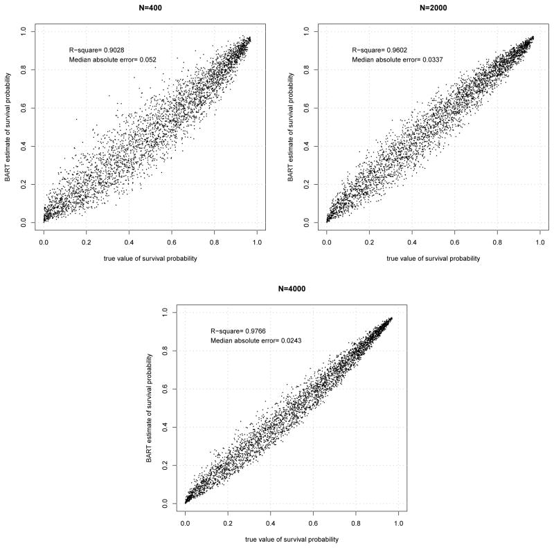
where x₁,...,x₅ are continuous covariates, each taking values in the unit interval. Adding five noise variables to these covariates, we simulated three data sets, with N = 400, 2000 and 4000. Each observation consisted of 10 independently generated covariates with uniform distributions on (0,1). Survival time was generated from the above Weibull distribution and right censored with an exponential variate to achieve an overall censoring rate of 20%. We applied the BART method to each data set and estimated the survival function at a grid of time points, made up of the 9 deciles of the overall survival function, for each 10-covariate combination in an independent sample of 400. Figure 5 shows estimated versus actual survival probabilities for the three data sets. Points are scattered nicely around the identity line in all cases with the larger sample sizes resulting in smaller variability. Together they indicate that BART fits well the complex functional relationship of covariates to survival probabilities.

Figure 5.

Plots of BART estimated survival probabilities vs true probabilities for the model with highly nonlinear relationship with covariates.

4.3. Application: hematopoietic stem cell transplantation data

In this section we apply the proposed BART survival method to a retrospective cohort study data set looking at survival after a reduced intensity hematopoietic cell transplant (HCT) from an unrelated donor [42] between the years 2000 to 2007. Patients with missing covariate data were removed to facilitate demonstration of the methods, so the results should be considered as an illustration of the methods rather than a clinical finding. A total of 592 deaths occurred in the 845 patients in the cohort. Thirteen covariates were considered in the analysis, including age, ABO blood type matching, year of transplant, disease/stage, human leukocyte antigen (HLA) matching, graft type, Karnofsky Performance Score (KPS), cytomegalovirus (CMV) status of the recipient, conditioning regimen, use of in vivo T-cell depletion, graft-versus-host disease (GVHD) prophylaxis, donor-recipient sex matching, and donor age, resulting in a total of 21 predictors in the X matrix. More details on the variables are available in [42]. The time scale was coarsened to weeks rather than days to reduce the computational burden.

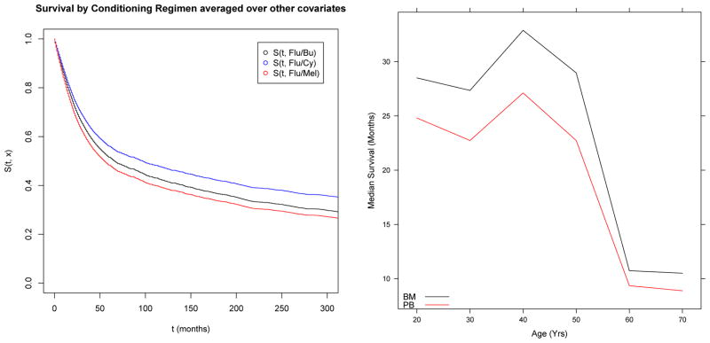
The BART survival model was fit to this data set with 200 trees and the default prior, using a burn-in of 100 draws and thinning by a factor of 10, resulting in 2000 draws from the posterior distributions for the survival function given covariates. Convergence diagnostics were carried out using generated values of p(t,x) = Φ(μ₀ + f(t,x)) at selected values of t and all x covariates at zero. While multiple chains converged quickly, sizable auto-correlation was observed and mitigated via thinning of the chain. Partial dependence survival functions can be obtained as in equation (6) for a particular subset of covariates. These can be interpreted as a marginal or average survival function for that covariate level, averaged across the observed distribution of the remaining covariates. In the left panel of Figure 6 we show the partial dependence survival function for each of three conditioning regimens.

Figure 6.

Left Panel: Partial Dependence Survival functions for 3 different conditioning regimens (Flu=Fludarabine, Bu=Busulfan, Cy=Cyclophosphamide, Mel=Melphalan); Right Panel: Median survival by age and graft type (BM= Bone Marrow, PB=Peripheral Blood)

One of the major advantages of the BART model is the ability to draw inference on various aspects of the survival distribution directly from the posterior samples. In the right panel of Figure 6 we examined how the median of the partial dependence survival function varied with patient age and graft type. There is little evidence of interaction as the plots are nearly parallel, and the plot indicates a nonlinear relationship between median survival and age, in which the median survival drops rapidly after age 50.

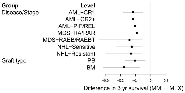
As another illustration of how one can use the BART survival model to explore interactions on different survival outcome scales, we examined the difference in the partial dependence survival function at 3 years between patients receiving MMF vs. MTX as GVHD prophylaxis, separately by disease status and by graft type. These are shown as a forest plot in Figure 7. These indicate MMF consistently reduces 3 year survival across different diseases and graft types, although the magnitude of the effect may vary slightly.

Figure 7.

Forest plot of the difference in 3 year survival between MMF(Mycophenalate Mofitol) and MTX(Methotrexate), separately by disease/stage (AML=Acute Myelogenous Leukemia, MDS=Myelodysplastic Syndrome, NHL=Non-Hodgkin’s Lymphoma, CR=Complete Remission, PIF=Primary Induction Failure, REL=Relapse, RA=Refractory Anemia, RAR=RA with Ringed Sideroblasts, RAEB=RA with Excess Blasts, RAEBT=RAEB in Transmission) and graft type (PB=Peripheral Blood, BM=Bone Marrow). Negative values indicate MMF has worse outcomes.

Finally, we applied the variable selection methods discussed in [35] by examining the average use per splitting rule for all 22 variables (time post transplant plus 21 predictors), plotted for several values for the number of trees used in the BART model (m = 200,100,50,40,30,20,15). Besides time post transplant, which is selected most consistently across the trees, the method identifies these 7 covariates impacting survival: patient age, disease/stage, HLA matching, KPS, conditioning regimen, and GVHD prophylaxis.

Additional variable selection methods using the average use per splitting rule are also available in [43] and described in Bleich et al. [44]. These include using permutation sampling to determine an appropriate threshold for the average use per splitting rule based on a null distribution which would help identify which variables are truly important.

5. Discussion

We have shown in the simulations and the application that BART can be successfully implemented in the nonparametric survival setting with or without covariates. In particular, we do not make any distributional assumptions or any assumptions about proportional hazards, so that the proposed method can fit complex nonlinear and interaction relationships of covariates in predicting or explaining survival time.

Our proposed method has good performance with respect to prediction error, consistent with prior studies of BART. As is well known, it is often informative to partition the mean square error into squared bias and variance to illuminate the trade-off between them. There are methods on both ends of the spectrum: linear regression, which has high bias and low variance; and CART, with low bias and high variance. Ensembles such as BART are generally in the middle: medium bias and medium variance. This unique placement in the trade-off spectrum accounts for the strong performance of ensembles from the standpoint of prediction error [45, 46, 47].

Our formulation allows for the use of “off-the-shelf” BART software after restructuring the data as described. R [48, 49] is a Free, Open Source Software (FOSS) language for statistical computing and graphics. Currently, there are three R packages available for BART which are also FOSS [40, 50, 43].

When modeling regression data, whether in the context of survival analysis or otherwise, model-building is a laborious process requiring much effort on the part of the analyst. Deciding which nonlinear relationships and interactions to include is a challenging task. BART and similar methods offer an alternative, that of a flexible modeling and prediction/estimation framework capable of discovering these complex relationships. One can obtain the posterior samples of ensembles of trees directly and then use these to understand the effect of various covariates on the outcome.

Many research studies suffer from missing data problems. While we did not address these directly in our study example, we point out that one of the BART implementations (bartMachine [43]) has a feature which allows the user to directly handle missing covariate data within the BART framework. This method incorporates missing data indicators into the training data set and allows for splits on the missing indicators, leading to improved performance under a pattern mixture model framework.

Beyond its many other advantages, BART is also an effective tool for causal inference of observational data with continuous outcomes as shown by Hill [51]. Specifically, BART has the advantage that only one model needs to be fit, as opposed to traditional propensity score analysis which requires separate models for treatment assignment and outcome. BART was more accurate than propensity score matching, weighting or regression adjustment when the scenario was non-linear; and competitive with propensity scores when the scenario was linear [51]. We believe that BART’s causal inference advantage over propensity scores is likely to be found in dichotomous and survival outcomes as well.

BART can be computationally demanding. This situation is aggravated in our case by expanding the data at a grid of event times. Luckily, BART, and MCMC in general, are considered to be “embarrassingly” parallel [52] since the chains do not share information besides the data itself, i.e., you can simultaneously perform calculations on m chains for a roughly linear (in m) improvement of processing time.

The computational burden can also be mitigated by coarsening the time scale, effectively changing its resolution (say from days to weeks). This induces more ties, reducing the number of distinct times used in constructing the grid. This is helpful particularly for large data sets, where the number of distinct times would be otherwise unwieldy. We are currently investigating alternative models which will not require such coarsening of the time measurement.

Finally, in the supplementary material, we provide an introduction to an ancillary R package that we have developed called survbart which is freely available online at http://survbart.r-forge.r-project.org. survbart includes R functions to prepare data (Section 2.1), to recover the survival function (Section 2.2) from the MCMC output produced by BayesTree [40] and to facilitate running BART in parallel on multiple cores. We also include R code illustrating an analysis of a publicly available data set.

References

- 1.Klein JP, van Houwelingen HC, Ibrahim JG, Scheike T. Handbook of Survival Analysis. Chapman & Hall; 2014. [Google Scholar]
- 2.Ibrahim JG, Chen MH, Sinha D. Bayesian Survival Analysis. Springer; 2001. [Google Scholar]
- 3.Klein JP, Moeschberger ML. Survival Analysis: Techniques for Censored and Truncated Data. Springer; 2003. [Google Scholar]
- 4.Andersen PK, Keiding N. Encyclopedia of Biostatistics. Wiley; 2005. Survival Analysis, Overview. [Google Scholar]
- 5.Hougaard P. Analysis of Multivariate Survival Data. Springer; 2000. [Google Scholar]
- 6.Kaplan EL, Meier P. Nonparametric estimation from incomplete observations. Journal of the American Statistical Association. 1958;53:457–481. [Google Scholar]
- 7.Ferguson TS, Phadia EG. Bayesian nonparametric estimation based on censored data. Annals of Statistics. 1979;7:163–186. [Google Scholar]
- 8.Dykstra RL, Laud PW. Bayesian nonparametric approach to reliability. Annals of Statistics. 1981;9:356–367. [Google Scholar]
- 9.Nelson W. Theory and applications of hazard plotting for censored failure data. Technometrics. 1972;14:945–965. [Google Scholar]
- 10.Brookmeyer R, Crowley JJ. A confidence interval for median survival time. Biometrics. 1982;38:29–41. [Google Scholar]
- 11.Peto R, Peto J. Asymptotically efficient rank invariant test procedures (with Discussion) Journal of the Royal Statistical Society, Series A. 1972;135:185–206. [Google Scholar]
- 12.Fleming TR, Harrington DP. A class of hypothesis tests for one and two samples of censored survival data. Communications in Statistics. 1981;10:763–794. [Google Scholar]
- 13.Pepe MS, Fleming TR. Weighted Kaplan-Meier statistics: a class of distance tests for censored survival data. Biometrics. 1989;45:497–507. [PubMed] [Google Scholar]
- 14.Cox DR. Regression models and life tables (with Discussion) Journal of the Royal Statistical Society, Series B. 1972;34:187–220. [Google Scholar]
- 15.Laud PW, Damien P, Smith AFM. Practical Nonparametric and Semiparametric Bayesian Statistics. In: Dey D, Müller P, Sinha D, editors. Bayesian nonparametric and covariate analysis of failure time data. Springer; 1998. pp. 213–225. [Google Scholar]
- 16.Ibrahim JG, Chen MH, Sinha D. Bayesian analysis of the Cox model. In: Klein JP, van Houwelingen HC, Ibrahim JG, Scheike T, editors. Handbook of Survival Analysis. Chapman & Hall; 2014. pp. 27–48. [Google Scholar]
- 17.Altman DG, Andersen PK. Bootstrap investigation of the stability of a Cox regression model. Statistics in Medicine. 1989;8:771–83. doi: 10.1002/sim.4780080702. [DOI] [PubMed] [Google Scholar]
- 18.Grambsch PM, Therneau TM. Proportional hazards tests and diagnostics based on weighted residuals. Biometrika. 1994;81:515–526. [Google Scholar]
- 19.O’Quigley J. Proportional Hazards Regression. Springer; 2008. [Google Scholar]
- 20.Martinussen T, Peng L. Alternatives to the Cox model. In: Klein JP, van Houwelingen HC, Ibrahim JG, Scheike T, editors. Handbook of Survival Analysis. Chapman & Hall; 2014. pp. 49–75. [Google Scholar]
- 21.Johnson W, Christensen R. Nonparametric Bayesian analysis of the accelerated failure time model. Statistics and Probability Letters. 1989;7:179–184. [Google Scholar]
- 22.DeIorio M, Johnson WO, Müller P, Rosner GL. Bayesian nonparametric nonproportional hazards survival modeling. Biometrics. 2009;65:762–771. doi: 10.1111/j.1541-0420.2008.01166.x. [DOI] [PMC free article] [PubMed] [Google Scholar]
- 23.Tibshirani R. The lasso method for variable selection in the Cox model. Statistics in Medicine. 1997;16:385–395. doi: 10.1002/(sici)1097-0258(19970228)16:4<385::aid-sim380>3.0.co;2-3. [DOI] [PubMed] [Google Scholar]
- 24.Park MY, Hastie T. L-1 regularization path algorithm for generalized linear models. Journal of the Royal Statistical Society, Series B. 2007;69:659–677. [Google Scholar]
- 25.Zhang HH, Lu W. Adaptive lasso for Cox’s proportional hazards model. Biometrika. 2007;94:691–703. [Google Scholar]
- 26.Li H, Luan Y. Boosting proportional hazards models using smoothing splines, with applications to high-dimensional microarray data. Bioinformatics. 2006;21:2403–2409. doi: 10.1093/bioinformatics/bti324. [DOI] [PubMed] [Google Scholar]
- 27.Li H, Luan Y. Clustering gradient descent regularization: with applications to microarray studies. Bioinformatics. 2006;23:466–472. doi: 10.1093/bioinformatics/btl632. [DOI] [PubMed] [Google Scholar]
- 28.Ishwaran H, Kogalur UB, Blackstone EH, Lauer MS. Random survival forests. Annals of Applied Statistics. 2008;2:841–860. [Google Scholar]
- 29.Breiman L, Friedman JH, Olshen R, Stone C. Classification and Regression Trees. Wadsworth; 1984. [Google Scholar]
- 30.Denison DGT, Mallick BK, Smith AFM. A Bayesian CART algorithm. Biometrika. 1998;85:363–377. [Google Scholar]
- 31.Chipman HA, George EI, McCulloch RE. Bayesian CART model search (with discussion) Journal of the American Statistical Association. 1998;93:935–60. [Google Scholar]
- 32.Breiman L. Random forests. Machine Learning. 2001;45:5–32. [Google Scholar]
- 33.Friedman JH. Greedy function approximation: a gradient boosting machine. Annals of Statistics. 2001;29:1189–1232. [Google Scholar]
- 34.Chipman HA, George EI, McCulloch RE. Bayesian treed models. Machine Learning. 2002;48:299–320. [Google Scholar]
- 35.Chipman HA, George EI, McCulloch RE. BART: Bayesian Additive Regression Trees. Annals of Applied Statistics. 2010;4:266–98. [Google Scholar]
- 36.Bonato V, Baladandayuthapani V, Broom BM, Sulman EP, Aldape KD, Do KA. Bayesian ensemble methods for survival prediction in gene expression data. Bioinformatics. 2011;27:359–367. doi: 10.1093/bioinformatics/btq660. [DOI] [PMC free article] [PubMed] [Google Scholar]
- 37.Gelfand AE, Smith AFM. Sampling-based approaches to calculating marginal densities. Journal of the American Statistical Association. 1990;85:398–409. [Google Scholar]
- 38.Fahrmeir L. Encyclopedia of Biostatistics. Wiley; 1998. Discrete survival-time models; pp. 1163–1168. [Google Scholar]
- 39.Albert J, Chib S. Bayesian analysis of binary and polychotomous response data. JASA. 1993;88:669–79. [Google Scholar]
- 40.Chipman H, McCulloch R. BayesTree: Bayesian Additive Regression Trees. 2014 [ http://lib.stat.cmu.edu/R/CRAN/web/packages/BayesTree/index.html]
- 41.Friedman JH. Multivariate adaptive regression splines (with discussion and a rejoinder by the author) Annals of Statistics. 1991;19:1–67. [Google Scholar]
- 42.Eapen M, Logan BR, Horowitz MM, Zhong X, Perales MA, Lee SJ, Rocha V, Soiffer RJ, Champlin RE. Bone marrow or peripheral blood for reduced intensity conditioning unrelated donor transplantation. Journal of Clinical Oncology. 2015;33:364–369. doi: 10.1200/JCO.2014.57.2446. [DOI] [PMC free article] [PubMed] [Google Scholar]
- 43.Kapelner A, Bleich J. bartMachine: Bayesian Additive Regression Trees. 2014 http://lib.stat.cmu.edu/R/CRAN/web/packages/[bartMachine/index.html]
- 44.Bleich J, Kapelner A, George EI, Jensen ST. Variable selection for BART: An application to gene regulation. The Annals of Applied Statistics. 2014;8(3):1750–1781. [Google Scholar]
- 45.Krogh A, Solich P. Statistical mechanics of ensemble learning. Physical Review E. 1997;55:811–25. [Google Scholar]
- 46.Baldi P, Brunak S. Bioinformatics: the machine learning approach. MIT Press; Cambridge, MA: 2001. [Google Scholar]
- 47.Kuhn M, Johnson K. Applied Predictive Modeling. Springer; New York, NY: 2013. [Google Scholar]
- 48.Ihaka R, Gentelman R. R: a language for data analysis and graphics. Journal of Computational and Graphical Statistics. 1996;5:299–314. [Google Scholar]
- 49.R Core Team. R: a language and environment for statistical computing. R Foundation for Statistical Computing; Vienna, Austria: 2014. [ http://www.R-project.org] [Google Scholar]
- 50.Chipman H, McCulloch R, Dorie V. dbarts: discrete Bayesian Additive Regression Trees sampler. 2014 http://lib.stat.cmu.edu/R/CRAN/web/[packages/dbarts/index.html]
- 51.Hill JL. Bayesian nonparametric modeling for causal inference. Journal of Computational and Graphical Statistics. 2011;20(1) [Google Scholar]
- 52.Rossini A, Tierney L, Li N. Technical Report. University of Washington; 2003. Simple parallel statistical computing in R. [ http://biostats.bepress.com/uwbiostat/paper193] [Google Scholar]
Associated Data
This section collects any data citations, data availability statements, or supplementary materials included in this article.