

Abstract
As the size of brain imaging data such as fMRI grows explosively, it provides us with unprecedented and abundant information about the brain. How to reduce the size of fMRI data but not lose much information becomes a more and more pressing issue. Recent literature studies tried to deal with it by dictionary learning and sparse representation methods, however, their computation complexities are still high, which hampers the wider application of sparse representation method to large scale fMRI datasets. To effectively address this problem, this work proposes to represent resting state fMRI (rs-fMRI) signals of a whole brain via a statistical sampling based sparse representation. First we sampled the whole brain’s signals via different sampling methods, then the sampled signals were aggregate into an input data matrix to learn a dictionary, finally this dictionary was used to sparsely represent the whole brain’s signals and identify the resting state networks. Comparative experiments demonstrate that the proposed signal sampling framework can speed-up by ten times in reconstructing concurrent brain networks without losing much information. The experiments on the 1000 Functional Connectomes Project further demonstrate its effectiveness and superiority.
Keywords: Resting state fMRI, sampling, DTI, DICCCOL, resting state networks
Introduction
With the advancement of neuroimaging technologies, the spatial and temporal resolution of brain imaging data such as fMRI has become higher and higher. For instance, the ongoing Human Connectome Project (HCP) (Van Essen et al. 2013) released its resting state fMRI (rs-fMRI) data with around 200,000 signals of 1200 time points. This fMRI big-data imposes significant challenges on the extraction and representation of neuroscientific meaningful information for human brain mapping. In response to this need, recently, sparse representation (Mairal et al. 2010; Wright et al. 2010) has been explored to represent whole-brain fMRI data and to reconstruct concurrent network activities (Oikonomou et al. 2012; Li et al. 2009; Eavani et al. 2012; Abolghasemi et al. 2013; Lv et al. 2014a; Li et al. 2012; Lee et al. 2011; Lv et al. 2014b). For example, Abolghasemi et al. 2013 adopted a fast incoherent K-SVD method for the detection of activated regions, and Eavani et al. utilized sparse representation method to identify highly modular, overlapping task-positive/negative pairs of functional sub-networks (Eavani et al. 2012). In particular, the recently developed holistic atlases of functional networks and interactions (HAFNI) system (Lv et al. 2014b) identified a number of reproducible and robust functional networks by sparse representation of whole-brain fMRI signals. The basic idea of HAFNI is that all fMRI signals within the whole brain of one subject were factorized into an over-complete basis signal dictionary and a reference coefficient matrix via dictionary learning and sparse coding algorithms (Mairal et al. 2010). Each dictionary atom represents the BOLD signal pattern of the functional activities of a specific brain network and its corresponding reference coefficient vector stands for the spatial distribution of this brain network (Lv et al. 2014a; Lv et al. 2014b).
However, these prior sparse representation methods still cost significant amount of time and memory space to learn a dictionary for one brain’s single fMRI scan because the input is a huge 4-D matrix with a number of over 106 voxels (several Giga bytes for the HCP fMRI images). The computing time cost thus would significantly hamper the wider application of sparse representation method to larger scale fMRI datasets. For instance, learning a dictionary for whole brain’s signals needs about 3,211 seconds, and loading a big fMRI data into memory needs more than 2 Giga Byte of space and about 900 seconds for merely one HCP rs-fMRI data on a usual laptop with Intel i5 3230 CPU. Therefore, this significant burden motivates us to investigate efficient data reduction methods, that is, signal sampling methods in this paper, to extract the representative signals without losing much information but can significantly speed-up. Our rationale is that the sampled fMRI signals can statistically and computationally well represent the original whole-brain fMRI data for concurrent brain network reconstruction based on prior successful applications of sampling methods in the statistical science fields (Meng et al. 2014; Mahoney 2011; Rao 2000).
Specifically, in this paper, we examined three rs-fMRI signal sampling methods, one is anatomical landmark-guided sampling by using the dense individualized and common connectivity-based cortical landmarks (DICCCOL) system (Zhu et al. 2013), and the other two are statistical random sampling and no sampling (using all of the whole brain’s signals) which are used for comparisons, respectively. The DICCCOL system consists of 358 consistent cortical landmarks, each of which has DTI-derived fiber connection pattern consistency across different subjects (Zhu et al. 2013). The DICCCOL system provide us the structural and functional correspondent cortical locations across different brains (Zhu et al. 2013), thus benefitting us to sample meaningful and functionally corresponding rs-fMRI signals across different subjects in this paper. This is also the technical contribution and novelty of this paper to adopt anatomical landmark to guide rs-fMRI signal sampling. The random sampling chooses each voxel randomly and entirely by chance (Yates et al. 2002; Tillé 2011). Since each voxel has the same probability of being chosen, it can be regarded as a comparable sampling method. Then the sampled signals are employed as an input to learn a dictionary (which is used to sparsely represent all signals) and corresponding sparse coefficient matrix (which gives the sparse weights for the combination of dictionary atom) by the online dictionary learning and sparse coding method (Mairal et al. 2010). Experimental results on reconstructing concurrent functional brain networks from the HCP rs-fMRI data show that DICCCOL-guided sampling is substantially better than statistical random sampling. In general, sampling 2% out of the 140,000–200,000 whole-brain signals is sufficient to learn an accurate dictionary for sparse representation and 10 times speed-up can be achieved in comparison with that using all of the whole brain’s signals.
Materials and Methods
Overview
Our framework of signal sampling for sparse representation of rs-fMRI data is summarized in Fig. 1. First, we sampled the rs-fMRI signal of the whole brain via the above three different sampling methods (DICCCOL-based sampling, random sampling, and no sampling). The bottom left of Fig. 1 shows the DICCCOL-based sampling locations of a brain as an example. Second, the sampled signals were used as an input matrix to learn an over-complete temporal dictionary via dictionary learning (Mairal et al. 2010). Third, the whole brain’s signals can be sparsely represented as a product of this dictionary and a sparse coefficient matrix by the sparse coding step (Mairal et al. 2010). Each row of the sparse coefficient matrix can be projected back to volumetric fMRI image space, resulting in the spatial maps of resting state networks (RSNs) of the brain (Fig. 1) for the interpretation of their spatial distributions. We described the dictionary learning and sparse coding theory in Section ‘dictionary learning and sparse representation’ and explained it in detail about the rationale of the proposed framework in section ‘DICCCOL-based sampling for sparse representation’ and Fig. 2. We compared and evaluated the temporal dictionary atoms and their spatial maps generated by the DICCCOL-guided sampling, random sampling, and no sampling, respectively, in the section of results.
Figure 1.

The overview of our computational framework. The sampling step represents DICCCOL-based sampling, statistical random sampling, or no sampling. The brain locations of DICCCOL-based sampling are shown in the bottom left corner as an example.
Figure 2.

(a) The illustration of dictionary learning and sparse representation. (b) Improved framework of dictionary learning and sparse representation with sampling. (c) One of DICCCOL landmarks (red planar triangles) and the corresponding fiber connections (white curves) from eight individuals.
Data acquisition and Preprocessing
The public HCP Q1 rs-fMRI dataset was used to explore and validate the proposed method. The acquisition parameters of rs-fMRI data were as follows: 2×2×2 mm spatial resolution, 0.72 s temporal resolution and 1200 time points. The L-R phase encoding rs-fMRI data of run 1 in HCP data was used in this paper. The preprocessing pipelines for rs-fMRI data included motion correction, spatial smoothing, temporal pre-whitening, slice time correction, global drift removal. The details of the HCP rs-fMRI dataset and preprocessing are referred to (Smith et al. 2013).
The HCP Q1 DTI data of the same subjects was also used for DICCCOL landmark system generation. The acquisition parameters of DTI data was acquired with the dimensionality of 144*168*110, space resolution 1.25mm*1.25mm*1.25mm, TR 5520ms and TE 89.5ms, with 90 DWI gradient directions and 6 B0 volumes acquired. Preprocessing of the DTI data included brain skull removal, motion correction, eddy current correction, tissue segmentation (Liu et al. 2007) and surface reconstruction (Liu et al. 2008). More details of the DTI dataset are referred to (Sotiropoulos et al. 2013). After the pre-processing, fiber tracking was performed using the MEDINRIA (FA threshold: 0.2; minimum fiber length: 20). Then, the DICCCOL landmarks were predicted based on the preprocessed DTI data according to the steps in our prior work (Zhu et al. 2013).
After preprocessing, rs-fMRI images were registered to its corresponding DTI space considering that since both DTI and rs-fMRI images use EPI (echo planar imaging) sequences, their geometric distortions tend to be similar, and their misalignment is much less (Li et al. 2010). Then the rs-fMRI signals are extracted based on any of the three sampling methods, and each signal was normalized to be with zero mean and standard deviation of 1 (Lv et al. 2014a).
Dictionary Learning and Sparse Representation
To decompose the fMRI signals and to identify the resting state networks (RSN) of human brain, we adopt a dictionary learning and sparse coding method (Abolghasemi et al. 2013; Lv et al. 2014a; Mairal et al. 2010) from the machine learning and pattern recognition fields. Briefly, it can be considered as a matrix factorization problem, given the sampled (based on any of the three sampling results) rs-fMRI signal matrix S∈ℝt×n. Here, each column represents an rs-fMRI signal time series and S can be factorized as S=D×A, where D∈ℝt×m is the dictionary, and A∈ℝm×n is called sparse coefficient matrix, as shown in Fig. 2(a). Each column in D is an atom of a learned basis dictionary D, and each rs-fMRI time series Si can be represented as a linear combination of atoms of dictionary, that is, Si = D × Ai, where Ai is a coefficient column in A which gives the sparse weights for the combination. Meanwhile, each row of the A matrix represents the spatial volumetric distributions that have references to certain dictionary atoms. In this work, the factorization problem was resolved by the publicly available effective online dictionary learning and sparse coding method (Mairal et al. 2010), which aims to learn a meaningful and over-complete dictionary of functional bases D∈ℝt×m (m>t, m≪n) for the sparse representation of S, and then to learn an optimized A matrix for spare representation of rs-fMRI time signal using the obtained dictionary matrix D.
To resolve this matrix factorization problem, Mairal et al. (Mairal et al. 2010) converted it to an empirical cost minimization function described in Equation (1) :
| (1) |
That means we should make the cost minimum meanwhile try to sparsely represent Si using D, thus leading to the following Equation (2):
| (2) |
Here, ℓ1 regularization yields a sparse resolution of Ai, and λ is a regularization parameter to trade-off the regression residual and sparsity level. Meanwhile, the dictionary atoms subject to the following constraints in Equation (3) since we mainly focus on the fluctuation shapes of basis fMRI activities and thus prevent D from arbitrarily large values:
| (3) |
More details for computing D are referred to (Mairal et al. 2010). Finally, when D is obtained, A is calculated as an l1-regularized linear least-squares problem (Mairal et al., 2010). In this way, the sampled rs-fMRI signals based on any of the three sampling methods are sparsely represented.
Different from other signal decomposition methods such as Independent Component Analysis (ICA) (McKeown et al., 1998), the superiority of sparse coding method is that it does not explicitly assume the independence of rs-fMRI signals among different components (Daubechies et al., 2009). The sparse coding method has been demonstrated to be effective and efficient in reconstructing concurrent spatially-overlapping functional networks (Lv et al. 2014a; Lv et al. 2014b). This finding is consistent with the current neuroscience knowledge that a variety of cortical regions and networks exhibit strong functional diversity and heterogeneity (Corbetta et al. 2008; Pessoa 2012), and that a cortical region could participate in multiple functional domains/processes and a functional network might recruit various heterogeneous neuroanatomic areas. Furthermore, the sparse representation framework can effectively achieve both compact high-fidelity representation of the whole-brain fMRI signals and effective extraction of meaningful patterns (Lv et al. 2014a; Lv et al. 2014b). Its data-driven strategy naturally accounts for that brain regions might be involved in multiple concurrent functional processes (corresponding to multiple dictionary atoms) (Corbetta et al. 2008; Gazzaniga 2004; Pessoa 2012; Duncan 2010) and thus their fMRI signals are composed of various intrinsic atoms (Varoquaux et al. 2011). Particularly its reference coefficient matrix naturally reveals the spatial interaction patterns among inferred brain networks (Lv et al. 2014a; Lv et al. 2014b).
Improved Framework of Dictionary Learning and Sparse Representation with Sampling
Based on the basic principle illustrated in Fig. 2(a), first, we sampled the whole brain’s signals via these three sampling methods, including DICCCOL-based sampling, random sampling and no sampling, respectively. Then, we aggregated the sampled signals into a signal matrix S′. In the second step, we employed the online dictionary learning and sparse coding method (Mairal et al. 2010) to learn the dictionary D′ and the corresponding coefficient matrix A′, that is S = D′ × A′. Finally, to obtain the sparse representation of whole brain signals, we performed the sparse coding method again on the whole brain signals matrix S using the learned D′ in this step, that is S = D′ × A, as shown in Fig. 2(b). Since learning D and A are two separate processes in the online dictionary learning and sparse coding algorithm (Mairal et al. 2010), we can combine the last two steps as one-time dictionary learning (obtaining D′) and one-time sparse coding (obtaining A), as shown in Fig. 2(b). In this way it does not induce additional computation in the algorithm.
The DICCCOL system (Zhu et al. 2013) provides a set of consistent cortical landmarks which have structural and functional correspondence across different subjects. These landmarks contain the key structural information of cortical regions and are naturally suitable for signal sampling. We first predicted the DICCCOL landmarks for the new dataset according to the measure of consistent fiber connection pattern (called trace-map, described in Zhu et al. 2013), these landmarks have similar fiber connection patterns across individuals, as shown in Fig 2(c). Then we extracted the n-ring surface neighborhood of all DICCCOL landmarks. Finally the rs-fMRI signals on all of these neighborhood voxels were extracted as sampling signals and were aggregated into a signal matrix S′. Here, we sampled the 0-ring, 2-ring, 4-ring and 6-ring neighborhood of DICCCOL landmarks.
In addition to the DICCCOL-based sampling, we also performed no sampling (using whole-brain signals, that is, S = D × A) and statistical random sampling (now S′ denotes the randomly sampled signals in Fig. 2(b)) for the purpose of comparison. To conduct a fair comparison, we sampled the same number of points with DICCCOL-based sampling for random sampling, that is, we sampled 358, 4709, 14199 and 25980 signals, corresponding to the number of signals of 0-ring, 2-ring, 4-ring and 6-ring DICCCOL sampling. Furthermore, we selected the same parameters for all of these three sampling methods, that is, the number of dictionary atom is 400, the sparsity regularization parameter λ=0.05, and set the batch size times iteration divided by the number of signals equals 4, and etc. The rationale of parameter selection is referred to literature reports (Mairal et al. 2010; Lv et al. 2014a).
Finally, we mapped each row in the A matrix back to the brain volume and examined their spatial distribution patterns, through which functional network components can be visualized and characterized on brain volumes. These network components are then identified as the known RSNs in the following section.
Identifying and Evaluating RSNs by Matching With Templates
To determine and evaluate the RSNs, we defined a metric named as Spatial Matching Ratio for checking the spatial similarity between the identified RSNs and the RSN template. In this work, we adopted the ten well-defined RSN templates provided in the literature (Smith et al. 2009). For the rs-fMRI data of each subject, we identified each RSN by matching its spatial weight map with each specific RSN template. Those network components with the maximum Spatial Matching Ratio (SMR) were selected as corresponding RSNs. The Spatial Matching Ratio is defined as follows:
| (4) |
where X is the spatial map of network component and T is the RSN template. |X ∩ T| and |X ∪ T| are the numbers of voxels in both X and T and in X or T, respectively. Notably, before the comparison of X and T, we registered all X images to T via the linear image registration method of FSL FLIRT.
Results and Discussion
By applying the DICCCOL sampling, random sampling and no sampling (Lv et al. 2014b) on 30 randomly selected subjects from the HCP datasets according to the procedure shown in Fig. 1, we generated their atomic dictionaries and corresponding coefficient matrices. For DICCCOL-based sampling, we sampled 0, 2, 4, 6 rings of points centered on DICCCOL landmarks, and they have 358, 4709, 14199, and 25980 rs-fMRI signals, respectively. For random sampling, we sampled the same number of points as corresponding n-ring DICCCOL-based sampling for the fairness of comparison and evaluation. Their results are as follows.
Comparison of Temporal Dictionary Atoms
To validate the effectiveness of the resulted dictionaries from the two sampling methods (DICCCOL-based and random sampling), we compared each dictionary atom with that of no sampling method. First, we identified the RSNs by matching them with the ten well-defined RSN templates (Smith et al. 2009). Those with the highest spatial matching ratio were selected out of the 400 network components as the RSNs. For the DICCCOL-based sampling, random sampling and whole brain signal without sampling, we performed the same identification procedure to find the most matched RSNs with the templates. Then we traced back to find the ten corresponding dictionary atoms associated with the ten identified RSNs. Thus we can compare the time series differences of the derived dictionaries by different sampling methods, as shown in Fig. 3. We quantitatively computed the Pearson correlation coefficients between the dictionaries by these sampling methods, as listed as in Table 1, and plotted the change curves of the averaged Pearson correlation coefficients on n rings (Fig. 4 (a)(b)). The blue and green ones are the Pearson correlation coefficients of DICCCOL-based sampling and random sampling, respectively.
Figure 3.


The time series signals of the 10 dictionary atoms resulted from DICCCOL-based sampling (blue curve), random sampling (green curve) and no sampling methods (red curve, as a baseline for comparison) from one randomly selected subject. For the convenience of inspect and limited space, only 200 time points are shown here, and only the atoms from 0-ring (a) and 6-ring (b) sampling are shown as examples. The blue curve represents the time series signal of atom from 0-ring (a)/6-ring (b) DICCCOL-based sampling. The green curve represents the time signals of atom generated by random sampling with the same number of points as n-ring DICCCOL-based sampling. WD/WR means the Pearson correlation coefficient between atom of whole brain and that of n-ring DICCCOL-based sampling/corresponding random sampling.
Table 1.
The Pearson correlations of 10 corresponding dictionary atoms between the two sampling methods and no sampling method. Each item was an averaged value from 30 subjects. “Dn” represents n-ring DICCCOL-based sampling and “Rn” represents sampling randomly the same number of points with the n-ring DICCCOL-based sampling.
| D0 | R0 | D2 | R2 | D4 | R4 | D6 | R6 | |
|---|---|---|---|---|---|---|---|---|
| atom0 | 0.7693 | 0.2772 | 0.7871 | 0.5021 | 0.7999 | 0.5438 | 0.8064 | 0.6007 |
| atom1 | 0.6261 | 0.2759 | 0.6405 | 0.4567 | 0.6644 | 0.4676 | 0.6707 | 0.5050 |
| atom2 | 0.6995 | 0.2747 | 0.7026 | 0.4846 | 0.7335 | 0.5936 | 0.7244 | 0.7293 |
| atom3 | 0.7337 | 0.3130 | 0.7423 | 0.4432 | 0.7547 | 0.5667 | 0.7560 | 0.6454 |
| atom4 | 0.5275 | 0.2886 | 0.5168 | 0.4474 | 0.5146 | 0.5116 | 0.5283 | 0.5180 |
| atom5 | 0.7515 | 0.3688 | 0.7591 | 0.5872 | 0.7685 | 0.7483 | 0.7700 | 0.7832 |
| atom6 | 0.6736 | 0.2886 | 0.6688 | 0.6017 | 0.6917 | 0.7174 | 0.6848 | 0.7259 |
| atom7 | 0.6131 | 0.2751 | 0.5968 | 0.5086 | 0.6078 | 0.5460 | 0.6198 | 0.6137 |
| atom8 | 0.5737 | 0.2942 | 0.5983 | 0.5163 | 0.6188 | 0.6923 | 0.6163 | 0.7784 |
| atom9 | 0.6740 | 0.2534 | 0.6931 | 0.4953 | 0.6948 | 0.5586 | 0.7445 | 0.6081 |
| Mean | 0.6642 | 0.2882 | 0.6705 | 0.5043 | 0.6849 | 0.5946 | 0.6921 | 0.6508 |
Figure 4.
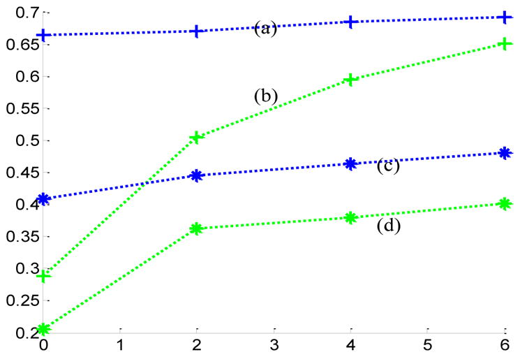
The change curves of the averaged Pearson correlation coefficients and Spatial Match Ratio on different rings of neighborhoods. (a) and (b) are the curves of the averaged Pearson correlation coefficients resulted from DICCCOL-based (blue curve) and random sampling (green one), respectively, their corresponding averaged SMR curves of RSNs are (c) and (d), respectively.
From Fig. 3, we can see that the atoms of DICCCOL-based sampling have much higher similarity with that of no sampling than random sampling, especially for the 0-ring DICCCOL-based sampling. As was also demonstrated by Table 1, the averaged Pearson correlation coefficients are 0.6642 and 0.2882, respectively. Meanwhile, we can see that for both DICCCOL-based and random sampling, the Pearson correlation coefficients are increased with the number of rings. It is reasonable considering that more sampled points contain more information. With the number of rings increasing, the Pearson correlation coefficients from random sampling increase fast. Random sampling and the DICCCOL-based sampling have almost the same high similarity (0.6921 vs 0.6508) with no sampling when n equals to 6. It was also shown in Fig. 3(b) and Figs. 4(a–b), but the Pearson correlation coefficients from 6-ring corresponding random sampling is still lower than that of 0-ring DICCCOL-based sampling (0.6508<0.6642). We checked their Spatial Match Ratio with the increment of rings in the next section and Fig. 4(c–d). However, we can see that the Pearson correlation coefficients from 6-ring DICCCOL-based sampling is lower than that from 0-ring DICCCOL-based sampling at specific situations, e.g., the two WDs of atom1 are 0.822 (0-ring) and 0.808 (6-ring) as shown in Fig. 3. Our explanation is that DICCCOL landmark itself provided more accurate information for atom 1, while its 6-ring neighborhood contains some other information different from atom 1. Regardless, on average, the Pearson correlation coefficients from 6-ring is larger than 0-ring DICCCOL-based sampling, as shown in Table 1 and Fig. 4(a–b).
In short, we can conclude that the dictionaries from DICCCOL-based sampling have substantially higher similarity with those of no sampling, compared with statistical random sampling. Therefore the dictionaries obtained by DICCCOL-based sampling are much more representative of the whole brain’s functional activities information. This result also suggests that DICCCOLs cover key functional areas of the brains, offering supporting evidence of the effectiveness and validity of the DICCCOL system (Zhu et al. 2013).
Comparison of Spatial RSNs
We identified 10 RSNs by matching each network component with 10 RSN templates (Smith et al. 2009), and performed this same step for the three sampling methods, respectively. Then we compared their spatial maps of the RSNs with 10 templates. The spatial maps from two randomly selected subjects and group-averaged maps were shown in Fig. 5, and for the convenience of checking and evaluating, these spatial maps were overlaid on MNI152 template images. Quantitatively, we computed the SMRs of RSNs with 10 templates, as shown in Table 2. We also plotted the change curves of SMRs on the number of rings, as shown in Fig. 4 (c) and (d).
Figure 5.


The spatial maps of RSNs by DICCCOL sampling, no sampling and the templates. In each panel of RSNs, the first row is the RSN template, the second row represents whole brain’s signals, the third and fourth one represent 0-ring DICCCOL sampling and corresponding random sampling with the same number of sampled points, respectively. The first and second columns are the results from two randomly selected subjects except the first row in each panel, which is putted there for the convenience of checking, and the third column shows the group-averaged results.
Table 2.
The SMR of 10 corresponding identified RSNs from the two sampling methods and no sampling method. “Dn” and “Rn” have the same meaning with that of Table 1, “W” means using whole brain’s signals (no sampling).
| W | D0 | R0 | D2 | R2 | D4 | R4 | D6 | R6 | |
|---|---|---|---|---|---|---|---|---|---|
| RSN0 | 0.624 | 0.611 | 0.291 | 0.626 | 0.421 | 0.679 | 0.438 | 0.700 | 0.463 |
| RSN1 | 0.522 | 0.431 | 0.222 | 0.544 | 0.391 | 0.546 | 0.389 | 0.544 | 0.396 |
| RSN2 | 0.435 | 0.387 | 0.205 | 0.417 | 0.405 | 0.443 | 0.444 | 0.497 | 0.473 |
| RSN3 | 0.454 | 0.401 | 0.157 | 0.448 | 0.400 | 0.470 | 0.411 | 0.502 | 0.409 |
| RSN4 | 0.429 | 0.194 | 0.178 | 0.450 | 0.238 | 0.491 | 0.297 | 0.322 | 0.315 |
| RSN5 | 0.504 | 0.487 | 0.198 | 0.434 | 0.454 | 0.389 | 0.431 | 0.565 | 0.494 |
| RSN6 | 0.748 | 0.455 | 0.149 | 0.388 | 0.321 | 0.459 | 0.267 | 0.507 | 0.356 |
| RSN7 | 0.421 | 0.341 | 0.246 | 0.231 | 0.350 | 0.207 | 0.351 | 0.222 | 0.389 |
| RSN8 | 0.304 | 0.371 | 0.254 | 0.465 | 0.274 | 0.484 | 0.296 | 0.463 | 0.294 |
| RSN9 | 0.408 | 0.373 | 0.293 | 0.417 | 0.348 | 0.435 | 0.353 | 0.473 | 0.363 |
| Mean | 0.493 | 0.409 | 0.219 | 0.445 | 0.362 | 0.463 | 0.369 | 0.480 | 0.399 |
We can see from Fig. 5 that the RSNs were successfully identified from both whole brain’s signals (no-sampling) and DICCCOL-based sampling. Moreover, the DICCCOL-based sampling has almost the same good results as those by no sampling method, which demonstrates that the rs-fMRI signals of DICCCOL-based sampling can well represent the rs-fMRI signal of the whole brain in terms of learning sparse dictionaries without losing much information. It has also been demonstrated in Table 2 that the SMR from DICCCOL-based sampling and whole brain’s signals have very close values. However, the random sampling method has much lower SMR, especially for the random sampling “R0” (358 sampled points) which have the same number of sampled points with 0-ring DICCCOL-based sampling. In order to check whether this difference/improvement obtained by DICCCOL-based sampling is significant compared with random sampling, we statistically analyzed the Pearson correlation and spatial matching ratio of these two group of sampling methods by one-tailed t-test, as shown in Figure 6. We can see that the difference is more significant when the number of sampling points is relatively small, and the two sampling method have no statistical difference when the number of sampling reaches 25980 (6-ring). Similarly, we can also see from Fig. 4 (c-d) that DICCCOL-based sampling achieved better performance than random sampling. Notably, all SMR values are not very high, even for the no sampling it is 0.493, since we identified these RSNs merely from 30 subjects while these templates were generated from about 30,000 brains (Smith et al. 2009). Therefore we check the two sampling methods with no sampling, not with the templates, and found that even for the 0-ring of sampling (358 points), the DICCCOL sampling (D0) achieved reasonably good accuracy (0.409 vs 0.493). It should be noted that the steep change occurs at the 2-ring DICCCOL sampling (Fig. 4 (c)), indicating that it might be a better choice when considering a trade-off between sampling size and accuracy.
Figure 6.

The statistical comparison between random sampling and DICCCOL-based sampling. The p values are shown on the top of bar only if p<0.05.
Comparison of Time Cost and Representation Error
Additionally, we evaluated and compared the computing time cost for dictionary learning, which is the major part of the online dictionary learning and sparse coding (Mairal et al. 2010) of different sampling methods. The dictionary learning step costs more time than the sparse coding step (whose time cost is fixed), and the difference of time cost heavily depends on the number of rs-fMRI signals given that the size of dictionary is fixed as 400. So we just computed and compared the time cost of dictionary learning. Each whole brain has about 2.4×10⁵ rs-fMRI signals, and a 0-ring, 2-ring, 4-ring and 6-ring DICCCOL-based sampling resulted in 358, 4709, 14199 and 25980 signals, accordingly, the random sampling have the same number of sampled points with n-ring DICCCOL sampling for the fairness of comparison. Their averaged time costs among 30 subjects were computed on a cluster with an Intel® Xeon CPU X5650, and the results are listed in the fourth row of Table 3. It is obvious that all sampling methods are faster than no sampling, especially for 2-ring DICCCOL-based sampling, it is approximately 10 times faster than no sampling without sacrificing much accuracy for sparsely representing the whole brain’s rs-fMRI signals.
Table 3.
The overall comparison of the three sampling methods. Each item is an averaged result among 30 subjects. For the convenience of overall comparison, the final results of Table 1 and 2 were also incorporated into Table 3. “W”, “Dn” and “Rn” have the same meaning with that of Table 1.
| W | D0 | R0 | D2 | R2 | D4 | R4 | D6 | R6 | |
|---|---|---|---|---|---|---|---|---|---|
| Pearson Correlation | N/A | 0.6642 | 0.2882 | 0.6705 | 0.5043 | 0.6849 | 0.5946 | 0.6921 | 0.6508 |
| SMR | 0.493 | 0.409 | 0.219 | 0.445 | 0.362 | 0.463 | 0.369 | 0.480 | 0.399 |
| Time Cost | 311.44s | 15.25s | 17.89s | 30.17s | 31.23s | 41.57s | 49.48s | 57.18s | 60.12s |
| Error | 0.629 | 2.245 | 5070.9 | 1.325 | 2.915 | 1.276 | 1.856 | 1.243 | 1.732 |
Furthermore, we computed the reconstruction/representation error of different sampling methods by the following expression (Mairal et al. 2010):
| (5) |
The results were list in the fifth row of Table 3, in which we can see that the almost all reconstruction error are tolerable except that of the 0-ring random sampling (having the same number with 0-ring DICCCOL sampling). This also demonstrated the effectiveness of sampling methods and dictionary learning and sparse coding (Abolghasemi et al. 2013).
Significant improvement of sampling-based method on fMRI Big Data
In order to inspect the significant improvement of sampling-based method on big data, especially for fMRI big data, we applied uniform sampling method on the 1000 Functional Connectomes Project (http://fcon_1000.projects.nitrc.org/), to test the time economy and accuracy for identifying the resting state networks. It is noted that due to the lack of DTI image in the 1000 Functional Connectomes Project dataset, DICCCOL-based sampling is not conducted in this subsection. The procedure of uniform sampling used in this subsection is primarily for the purpose of testing whether/how sampling significantly speed-ups sparse coding of rs-fMRI big data and of course other types of sampling methods could be explored in the future. The 1000 Functional Connectomes Project is a collection of resting-state fMRI datasets from more than 1000 subjects, and thus this large resting-state data offers the unique opportunity to study resting state networks at both subject and study level (Yan et al. 2013; Kalcher et al. 2012). We used the uniform sampling as an example to identify the resting state networks, and compared its time cost with no sampling method, by performing the codes on our Hafni-Enabled Largescale Platform for Neuroimaging Informatics (HELPNI), which is an integrated solution to archive and manage primary and processed data as well as to analyze and to process large scale data automatically and structurally. The average time of obtaining the dictionary for one brain is about 1.05 seconds using uniform sampling method, whereas the time cost is 11.17 seconds for no sampling method. We can see that the sampling-based method can bring around ten times speed-up, this will save much time when the subject number is 1000 and even more, such as the 1000 Functional Connectomes Project. It is significant improvement when we intend to find out interesting information from fMRI big data and it is exactly the meaning of big data. Notably, for a fair comparison, we counted the time cost by running the program on only one CPU core (Intel® Xeon® E5-2650 v2 2.60GHz).
We further checked the spatial maps with sampling method. The identified 10 group-wise resting state networks from the 5 randomly selected datasets by the sampling-based method are shown in Fig. 7. Fig. 8 illustrates the individual resting state networks from a randomly select subject of the 5 datasets. From Fig. 7 and Fig. 8, we can see that the identified ten RSN networks are quite consistent with the ten templates (Smith et al. 2009). Quantitative measurement between the identified resting networks and templates are shown in Table 4 and Table 5. From these results, we can see that the sampling-based method is effective and feasible. The sampling-based method on fMRI big data shows significant speedup and comparable results.
Figure 7.

The ten group-wise RSN networks from 5 randomly select datasets (Baltimore, Beijing, Berlin, Cambridge and Cleveland) in 1000 Functional Connectomes Project, identified by the 2-ring DICCCOL-based sampling method. The second row shows the RSN templates for comparison and the following rows show the identified group-wise networks from different datasets.
Figure 8.

The individual RSN networks identified by the 2-ring DICCCOL-based sampling method, one randomly selected subject for each dataset.
Table 4.
Spatial match ratio between identified group-wise RSN networks by DICCCOL sampling method and template for different datasets.
| RSN1 | RSN2 | RSN3 | RSN4 | RSN5 | RSN6 | RSN7 | RSN8 | RSN9 | RSN10 | |
|---|---|---|---|---|---|---|---|---|---|---|
| Baltimore | 0.58 | 0.59 | 0.30 | 0.42 | 0.56 | 0.30 | 0.42 | 0.34 | 0.32 | 0.44 |
| Beijing | 0.52 | 0.59 | 0.27 | 0.46 | 0.59 | 0.22 | 0.51 | 0.32 | 0.38 | 0.38 |
| Berlin | 0.42 | 0.33 | 0.25 | 0.40 | 0.56 | 0.20 | 0.47 | 0.34 | 0.22 | 0.29 |
| Cambridge | 0.58 | 0.62 | 0.33 | 0.52 | 0.44 | 0.27 | 0.57 | 0.39 | 0.48 | 0.48 |
| Cleveland | 0.47 | 0.50 | 0.25 | 0.40 | 0.55 | 0.19 | 0.46 | 0.35 | 0.29 | 0.37 |
Table 5.
Spatial match ratio between identified individual RSN networks by DICCCOL sampling method and templates for different datasets. Represented as MEAN±STD.
| RSN1 | RSN2 | RSN3 | RSN4 | RSN5 | RSN6 | RSN7 | RSN8 | RSN9 | RSN10 | |
|---|---|---|---|---|---|---|---|---|---|---|
| Baltimore | 0.25±0.06 | 0.17±0.05 | 0.11±0.03 | 0.19±0.03 | 0.17±0.03 | 0.12±0.04 | 0.12±0.03 | 0.14±0.03 | 0.12±0.02 | 0.13±0.03 |
| Beijing | 0.19±0.06 | 0.16±0.06 | 0.11±0.03 | 0.18±0.04 | 0.16±0.03 | 0.10±0.02 | 0.16±0.04 | 0.14±0.04 | 0.13±0.03 | 0.13±0.03 |
| Berlin | 0.20±0.04 | 0.15±0.05 | 0.09±0.04 | 0.19±0.04 | 0.15±0.03 | 0.11±0.02 | 0.15±0.03 | 0.16±0.03 | 0.12±0.02 | 0.13±0.03 |
| Cambridge | 0.24±0.05 | 0.19±0.06 | 0.12±0.03 | 0.20±0.04 | 0.18±0.03 | 0.13±0.03 | 0.17±0.03 | 0.19±0.03 | 0.14±0.03 | 0.14±0.03 |
| Cleveland | 0.20±0.08 | 0.16±0.07 | 0.09±0.03 | 0.17±0.03 | 0.12±0.04 | 0.11±0.02 | 0.14±0.03 | 0.16±0.04 | 0.15±0.03 | 0.12±0.03 |
Conclusion
In this paper, we presented and evaluated a novel signal sampling strategy for efficient sparse representation of rs-fMRI data. We quantitatively and qualitatively compared three sampling schemes and experimental results demonstrated that the DICCCOL-based sampling signals exhibit much better performance than statistical random sampling for identifying RSNs, and have almost the same high performance as no sampling method. Also, the signal sampling method achieved around ten times speed-up. Thus, we can conclude that DICCCOL-based sampling is able to well represent the whole brain’s rs-fMRI signals with lower cost. However, we agree that there are still some other advanced statistical sampling methods which were not compared with DICCCOL-based sampling in this stage. Our main purpose was not to demonstrate DICCCOL-based sampling is the best, but rather that it has enough accuracy and good speed-up. More importantly, it provides us with important structural information, which is beneficial to our later works, for example, we can further decrease the number of sampling points and find out which DICCCOL landmarks are more important for constructing resting state networks and which are more crucial for constructing task-evoked network. However, the statistical methods cannot provide comparable structural information and cannot combine function with structure of the brain. It is of important significance for brain imaging big-data to reduce the data size but not to lose much information, because a 4-D fMRI data needs very much time and memory space to be processed if there’s no efficient sampling method, we made the initial effort to deal with this challenge via the different sampling methods in this paper, and we expect more and more sampling methods for brain imaging big data could be explored. For instance, in the future, we plan to explore other statistically-principled sampling methods such as the leverage score based sampling methods (Meng et al. 2014; Mahoney 2011; Ma et al. 2015) and other dictionary learning algorithms such as Stochastic Coordinate Coding (Lin et al. 2014) combined with DICCCOL-based sampling to represent rs-fMRI information of brain more efficiently, and apply and evaluate them on more fMRI datasets.
Acknowledgments
We thank all investigators contributing data to the 1000 Functional Connectomes project, without whom this analysis could not have been performed. T Liu was supported by NIH R01 DA-033393, NIH R01 AG-042599, NSF CAREER Award IIS-1149260, NSF CBET-1302089 and NSF BCS-1439051. B Ge was supported by NSFC 61403243, 2015JM6312, the Fundamental Research Funds for the Central Universities from China (No. GK201402008) and Interdisciplinary Incubation Project of Learning Science of Shaanxi Normal University. The authors would like to thank the anonymous reviewers for their constructive comments.
Footnotes
Conflict of Interest: None of the authors has conflict of interest to declare.
Compliance with Ethical Standards
Ethical approval: This article does not contain any studies with animals performed by any of the authors.
Ethical approval: This article does not contain any studies with human participants or animals performed by any of the authors.
References
- Abolghasemi V, Ferdowsi S, Sanei S. Fast and incoherent dictionary learning algorithms with application to fMRI. Signal, Image and Video Processing. 2013:1–12.
- Corbetta M, Patel G, Shulman GL. The reorienting system of the human brain: from environment to theory of mind. Neuron. 2008;58(3):306–324. doi: 10.1016/j.neuron.2008.04.017. [DOI] [PMC free article] [PubMed] [Google Scholar]
- Daubechies I, Roussos E, Takerkart S, Benharrosh M, Golden C, D’Ardenne K, Richter W, Cohen JD, Haxby J. Independent component analysis for brain fMRI does not select for independence. Proceedings of the National Academy of Sciences. 2009;106(26):10415–10422. doi: 10.1073/pnas.0903525106. [DOI] [PMC free article] [PubMed] [Google Scholar]
- Duncan J. The multiple-demand (MD) system of the primate brain: mental programs for intelligent behaviour. Trends Cogn Sci. 2010;14(4):172–179. doi: 10.1016/j.tics.2010.01.004. [DOI] [PubMed] [Google Scholar]
- Eavani H, Filipovych R, Davatzikos C, Satterthwaite TD, Gur RE, Gur RC. Sparse dictionary learning of resting state fMRI networks. Int Workshop Pattern Recognit Neuroimaging. 2012:73–76. doi: 10.1109/PRNI.2012.25. [DOI] [PMC free article] [PubMed] [Google Scholar]
- Gazzaniga MS. The cognitive neurosciences. MIT press; 2004. [Google Scholar]
- Huang K, Aviyente S. Sparse representation for signal classification. Advances in Neural Information Processing Systems. 2006:609–616. [Google Scholar]
- Kalcher K, Huf W, Boubela RN, Filzmoser P, Pezawas L, Biswal B, et al. Fully exploratory network independent component analysis of the 1000 functional connectomes database. Front Hum Neurosci. 2012;6:301. doi: 10.3389/fnhum.2012.00301. [DOI] [PMC free article] [PubMed] [Google Scholar]
- Lee K, Tak S, Ye JC. A Data-Driven Sparse GLM for fMRI Analysis Using Sparse Dictionary Learning With MDL Criterion. IEEE Trans Med Imaging. 2011;30(5):1076–1089. doi: 10.1109/Tmi.2010.2097275. [DOI] [PubMed] [Google Scholar]
- Li K, Guo L, Li G, Nie J, Faraco C, Zhao Q, et al. Cortical surface based identification of brain networks using high spatial resolution resting state FMRI data. Biomedical Imaging: From Nano to Macro; 2010 IEEE International Symposium on; 2010; IEEE; pp. 656–659. [Google Scholar]
- Li Y, Long J, He L, Lu H, Gu Z, Sun P. A sparse representation-based algorithm for pattern localization in brain imaging data analysis. PLoS One. 2012;7(12):e50332. doi: 10.1371/journal.pone.0050332. [DOI] [PMC free article] [PubMed] [Google Scholar]
- Li Y, Namburi P, Yu Z, Guan C, Feng J, Gu Z. Voxel selection in fMRI data analysis based on sparse representation. Biomedical Engineering, IEEE Transactions on. 2009;56(10):2439–2451. doi: 10.1109/TBME.2009.2025866. [DOI] [PubMed] [Google Scholar]
- Lin B, Li Q, Sun Q, Lai M-J, Davidson L, Fan W, et al. Stochastic Coordinate Coding and Its Application for Drosophila Gene Expression Pattern Annotation. 2014 arXiv:1407.8147v2 [cs.LG] [Google Scholar]
- Liu T, Li H, Wong K, Tarokh A, Guo L, Wong ST. Brain tissue segmentation based on DTI data. Neuroimage. 2007;38(1):114–123. doi: 10.1016/j.neuroimage.2007.07.002. [DOI] [PMC free article] [PubMed] [Google Scholar]
- Liu T, Nie J, Tarokh A, Guo L, Wong STC. Reconstruction of central cortical surface from brain MRI images: method and application. Neuroimage. 2008;40(3):991–1002. doi: 10.1016/j.neuroimage.2007.12.027. [DOI] [PMC free article] [PubMed] [Google Scholar]
- Lv J, Jiang X, Li X, Zhu D, Chen H, Zhang T, et al. Sparse representation of whole-brain fMRI signals for identification of functional networks. Med Image Anal. 2014a doi: 10.1016/j.media.2014.10.011. [DOI] [PubMed] [Google Scholar]
- Lv J, Jiang X, Li X, Zhu D, Zhang S, Zhao S, et al. Holistic Atlases of Functional Networks and Interactions Reveal Reciprocal Organizational Architecture of Cortical Function. IEEE Trans Biomed Eng. 2014b doi: 10.1109/TBME.2014.2369495. [DOI] [PubMed] [Google Scholar]
- Ma P, Mahoney MW, Yu B. A statistical perspective on algorithmic leveraging. Journal of Machine Learning Research. 2015;16:861–911. [Google Scholar]
- Mahoney MW. Randomized algorithms for matrices and data. Foundations and Trends® in Machine Learning. 2011;3(2):123–224. [Google Scholar]
- Mairal J, Bach F, Ponce J, Sapiro G. Online Learning for Matrix Factorization and Sparse Coding. Journal of Machine Learning Research. 2010;11:19–60. [Google Scholar]
- McKeown MJ, et al. Spatially independent activity patterns in functional MRI data during the Stroop color-naming task. PNAS. 1998;95(3):803. doi: 10.1073/pnas.95.3.803. [DOI] [PMC free article] [PubMed] [Google Scholar]
- Meng X, Saunders MA, Mahoney MW. LSRN: A parallel iterative solver for strongly over-or underdetermined systems. SIAM Journal on Scientific Computing. 2014;36(2):C95–C118. doi: 10.1137/120866580. [DOI] [PMC free article] [PubMed] [Google Scholar]
- Oikonomou VP, Blekas K, Astrakas L. A sparse and spatially constrained generative regression model for fMRI data analysis. IEEE Trans Biomed Eng. 2012;59(1):58–67. doi: 10.1109/TBME.2010.2104321. [DOI] [PubMed] [Google Scholar]
- Pessoa L. Beyond brain regions: Network perspective of cognition-emotion interactions. Behavioral and Brain Sciences. 2012;35(3):158–159. doi: 10.1017/S0140525x11001567. [DOI] [PubMed] [Google Scholar]
- Rao P. Sampling methodologies with applications. Chapman & Hall/CRC; 2000. [Google Scholar]
- Smith SM, Beckmann CF, Andersson J, Auerbach EJ, Bijsterbosch J, Douaud G, et al. Resting-state fMRI in the Human Connectome Project. Neuroimage. 2013;80:144–168. doi: 10.1016/j.neuroimage.2013.05.039. [DOI] [PMC free article] [PubMed] [Google Scholar]
- Smith SM, Fox PT, Miller KL, Glahn DC, Fox PM, Mackay CE, et al. Correspondence of the brain’s functional architecture during activation and rest. Proc Natl Acad Sci U S A. 2009;106(31):13040–13045. doi: 10.1073/pnas.0905267106. [DOI] [PMC free article] [PubMed] [Google Scholar]
- Sotiropoulos SN, Moeller S, Jbabdi S, Xu J, Andersson JL, Auerbach EJ, et al. Effects of Image Reconstruction on Fiber Orientation Mapping From Multichannel Diffusion MRI: Reducing the Noise Floor Using SENSE. Magnetic Resonance in Medicine. 2013;70(6):1682–1689. doi: 10.1002/Mrm.24623. [DOI] [PMC free article] [PubMed] [Google Scholar]
- Tillé Y. Sampling algorithms. Springer; 2011. [Google Scholar]
- Van Essen DC, Smith SM, Barch DM, Behrens TE, Yacoub E, Ugurbil K. The WU-Minn Human Connectome Project: an overview. Neuroimage. 2013;80:62–79. doi: 10.1016/j.neuroimage.2013.05.041. [DOI] [PMC free article] [PubMed] [Google Scholar]
- Varoquaux G, Gramfort A, Pedregosa F, Michel V, Thirion B. Multi-subject dictionary learning to segment an atlas of brain spontaneous activity. Inf Process Med Imaging. 2011;22:562–573. doi: 10.1007/978-3-642-22092-0_46. [DOI] [PubMed] [Google Scholar]
- Wright J, Ma Y, Mairal J, Sapiro G, Huang TS, Yan SC. Sparse Representation for Computer Vision and Pattern Recognition. Proceedings of the Ieee. 2010;98(6):1031–1044. doi: 10.1109/Jproc.2010.2044470. [DOI] [Google Scholar]
- Yan CG, Craddock RC, Zuo XN, Zang YF, Milham MP. Standardizing the intrinsic brain: towards robust measurement of inter-individual variation in 1000 functional connectomes. Neuroimage. 2013;80:246–262. doi: 10.1016/j.neuroimage.2013.04.081. [DOI] [PMC free article] [PubMed] [Google Scholar]
- Yang M, Zhang L, Feng XC, Zhang D. Sparse Representation Based Fisher Discrimination Dictionary Learning for Image Classification. International Journal of Computer Vision. 2014;109(3):209–232. doi: 10.1007/s11263-014-0722-8. [DOI] [Google Scholar]
- Yates D, Moore DS, Starnes DS. The practice of statistics: TI-83/89 graphing calculator enhanced. Macmillan; 2002. [Google Scholar]
- Zhu D, Li K, Guo L, Jiang X, Zhang T, Zhang D, et al. DICCCOL: dense individualized and common connectivity-based cortical landmarks. Cereb Cortex. 2013;23(4):786–800. doi: 10.1093/cercor/bhs072. [DOI] [PMC free article] [PubMed] [Google Scholar]