Tree-structured supervised learning and the genetics of hypertension

Abstract

This paper is about an algorithm, FlexTree, for general supervised learning. It extends the binary tree-structured approach (Classification and Regression Trees, CART) although it differs greatly in its selection and combination of predictors. It is particularly applicable to assessing interactions: gene by gene and gene by environment as they bear on complex disease. One model for predisposition to complex disease involves many genes. Of them, most are pure noise; each of the values that is not the prevalent genotype for the minority of genes that contribute to the signal carries a “score.” Scores add. Individuals with scores above an unknown threshold are predisposed to the disease. For the additive score problem and simulated data, FlexTree has cross-validated risk better than many cutting-edge technologies to which it was compared when small fractions of candidate genes carry the signal. For the model where only a precise list of aberrant genotypes is predisposing, there is not a systematic pattern of absolute superiority; however, overall, FlexTree seems better than the other technologies. We tried the algorithm on data from 563 Chinese women, 206 hypotensive, 357 hypertensive, with information on ethnicity, menopausal status, insulin-resistant status, and 21 loci. FlexTree and Logic Regression appear better than the others in terms of Bayes risk. However, the differences are not significant in the usual statistical sense.

As interest in complex disease increases, there is increasing need for methodologies that address issues such as gene–gene and gene–environment interactions in a robust fashion. We report on a binary tree-structured classification tool, FlexTree, that addresses such needs. Our principal application has been to predict a complex human disease (hypertension) from single-nucleotide polymorphisms (SNPs) and other variables. FlexTree extends the approach of Classification and Regression Trees (CART; ref. 1); it retains CART's simple binary tree structure. However, it differs in its ability to handle combinations of predictors. Furthermore, the construction of the tree respects family structures in the data. FlexTree involves coding categorical predictors to indicator variables, suitably scoring outcomes, backward selection of predictors by importance estimated from the bootstrap, and then borrowing from CART (1). We convert a problem of classification to one of regression without losing sight of classification. The approach we take resembles that of Zhang (2), although his focus is on different criteria for splitting, and he seems not to be concerned as we are about shaving the list of candidate features at each node. Each vector of predictor values can be located to a terminal node of the tree. Finding groups with high risk of disease may lend understanding to etiology and genetic mechanism. In most applications of classification trees, each split is on one feature. This seems inappropriate for polygenic disease, when no single gene is decisive, and the “main effect” may be a gene by environment interaction. With FlexTree as applied to data concerning certain Asian women (which will be described), we suggest complicated associations of hypertension and predictors. They include insulin resistance, menopausal status, and SNPs in a protein tyrosine phosphatase gene and the mineralocorticoid receptor gene. A particular strength of the approach taken here, as opposed to the approaches that involve schemes for voting among predictors or random selection of features, is its ability to make simple, clear choices of relevant features at each node. In particular, we find predictive, simple linear combinations of features, and we get at the issue of each genotype's being predictive or a risk factor for an untoward outcome.

Algorithm

FlexTree borrows strength from both classification trees and regression; it creates a simple rooted binary tree with each split defined by a linear combination of selected variables. The linear combination is achieved by regression with optimal scoring. The variables are selected by a backward shaving procedure. Using a selected variable subset to define each split increases interpretability, improves robustness of the prediction, and prevents overfitting. FlexTree deals with additive and interactive effects simultaneously. Sampling units can be families or individuals, depending on the application.

Data Transformation. In the situation of finding influential genes for a polygenic disease, the outcome is dichotomous disease status, affected versus disease-free, and the predictors are mutations at different loci. They are all qualitative. The response variable Ỹ with L₀ unordered classes and N observations is changed to an N by L₀ dummy matrix with elements 0 or 1: Ỹ ⇒ Y_N×L0. Each observation is transformed to an L₀-dimensional indicator vector:

[1]

[2]

A predictor with K levels is represented by K – 1 instead of K columns in the design matrix to avoid singularity. One level of each variable is chosen as the baseline with the corresponding column removed. With J nominal categorical predictors X̃_j, 1 ≤ j ≤ J, each having N observations and L_j categories, the design matrix X is X = (1, X₁, X₂,..., X_J) = X_N×M, where M = 1 +Σ(L_j –1) = ΣL_j – J + 1. This coding scheme is similar to but in fact more general than that of Zhang and Bonney (3).

Regression and the Splitting Criteria. The regression framework is built on the transformed data. The binary splitting rule is defined as an inequality involving a linear combination of a subset of the predictors: X_selectβ ≥ C. The problem of classification is thus transformed to one of regression. Optimal scoring can be viewed as an asymmetric version of canonical correlation analysis and linear discriminant analysis (4). The optimal scores Θ=Θ_{L0 ×1} = (θ₁, θ₂,..., θ_L0)^T are determined as those that minimize the penalized sum of squares

[3]

under the constraint ∥YΘ∥²/N = 1. Ω is a penalty term introduced to avoid singularity, which occurs when there are many predictors involved or in the later stages of the partitioning, where the sample within a node is deliberately homogeneous. Ω = λI, where we have taken λ = 0.001 in our computations, although obviously there could be other choices. Our motivation to use optimal scoring as a component of the algorithm is supported by findings of Hastie et al. (ref. 5, section 12.5.1). For any given score Θ, the penalized least-squares estimate of β is

[4]

Substitute Eq. 4 into formula 3, and the formula simplifies to

[5]

Θ that minimizes formula 5 is the eigenvector corresponding to the largest eigenvalue of the matrix.

[6]

Θ is standardized to satisfy ∥YΘ∥²/N = 1. After the optimal scores are obtained, linear regression of the quantified outcome Z on X is applied:

[7]

[8]

is minimized, which entails estimated regression coefficients and outcome

[9]

[10]

When X is full rank, simple linear regression is applied without a penalty term. A binary split is defined as . C is chosen to maximize the impurity reduction

[11]

where R_t indicates the weighted generalized Gini index for the current node t; R_l is one for the left daughter node of a given partition; and R_r is the one for the right daughter node (1). One critical question concerns how to choose the right subset of predictors on which to perform the regression. Another is how to measure the relative importance of each predictor involved.

“Backward Shaving” and Node-Specific Variable Ranking. Backward shaving begins with the full set of predictors. Selected proportions of them are successively shaved off until only a single predictor remains. This procedure produces nested families of predictors, from the full set to a single one. The shaving is based on the node-specific variable ranking defined by bootstrapped p values. Such p values are derived from a χ² statistic as it applies to testing the null hypothesis that “related” regression coefficients are all zero:

[12]

Here β_(Xi) indicates the subset of regression coefficients for predictor X_i. 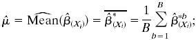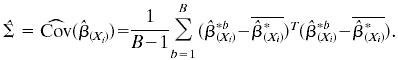We assume (without obvious loss) that the outcome is calculated as the appropriate entry in a vector of “optimal” scores, which are the coordinates of the first canonical variable that relates outcome and predictors, and , the least-squares estimate of β_(Xi), has approximately a multinormal distribution , which implies that the solid ellipsoid of Z values satisfying has probability about 1 – α. We use the bootstrap to estimate μ and Σ and to evaluate variable importance. Observations are often correlated, and the predictors can be categorical. We first bootstrap families (or individuals, as the case may be) to obtain B independent bootstrap samples (X*¹, Y*¹), (X*², Y*²),..., (X*^B, Y*^B). For each sample (X*^b, Y*^b), we estimate the optimal score Θ*^b and the regression coefficients as described in the previous section. We then compute the sample mean and sample covariance of , from the B bootstrapped estimates to B:

[13]

[14]

Given , and , the test statistic is

[15]

which has approximately a distributionl under the multinormal approximation. The p value derived from this test statistic corresponds to the 100(1 – p)% ellipsoid-confidence-contour, where the boundary goes through the origin. In what follows, this is referred to as the T² p value. These p values give not only a measure of variable importance but also an order for shaving. We repeatedly shave off a certain number of “least important” variables until only the single most important variable is left, and create a nested sequence of variable subsets:

[16]

The subset S₁ = S^(i₁) that includes the least number of variables and yet achieves approximately the largest impurity reduction within a prespecified error margin is chosen. The error margin is set to be 5% of the largest impurity reduction.

[17]

Variables that are not included in S₁ are shaved off. In the case where S₁ = S^(m), the least significant variable is shaved off to keep the process going. Then S₁ is treated as the full set, and the shaving procedure is repeated with new optimal scores to get an even smaller set. The procedure is continued until only one variable is left. This again gives us a sequence of nested variable subsets, full set = S₀ ⊃ S₁ ⊃ S₂ ⊃ ... ⊃ S_h–1 ⊃ S_h = a single variable.m The optimal subset is determined by the mean of the cross-validated estimates; k-fold cross-validation (k = 5 or 10) is applied to each set in the nested sequence to estimate the impurity reduction associated with the subset.

[18]

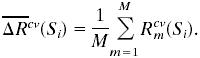
where R_t is the impurity measure of the current node t according to the cross-validated partition rule using variable subset S_i; is the impurity measure of the left daughter node; R^cv_tr(S_i) is the impurity measure of the right daughter node. Because single cross-validation is relatively unstable, it is repeated M = 40 times, each time with a different k-nary partition of the data. The means of the M cross-validated estimates quantify the performance of each subset:

[19]

The subset with the largest mean (within 1 SE) is chosen as the final variable subset to define the binary split. After the final set is chosen, a permutation t test on the quantity given by Eq. 18 is performed to test whether there is any (linear) association between the outcome and the selected predictors. If the test statistic is larger than a preassigned threshold, we conclude there is still significant association and continue splitting the node. Otherwise, we stop. Beyond this subsidiary stopping rule, procedures for growing and pruning trees are exactly as in CART.

Missing Value Imputation. Genetic data are prone to problems with missing values. To avoid losing valuable information, we try to retain observations with some missing values in the analysis. Because genetic predictors are often at least moderately correlated, we use these correlations at least implicitly to establish a predictive model for the one with missing values, using all of the other predictors. In particular, we chose the standard classification tree method to serve as such a predictive model. It is flexible, being applicable to both categorical and continuous variables without distributional assumptions. Also, it deals with missing values effectively through surrogate splits and can succeed in situations where many predictors in the training set have missing values (5). Strictly speaking, our imputation scheme is valid only if data are “missing at random.”

Testing Association, Genotype by Disease Status. Given a SNP with three genotypes and disease status (yes or no) for each subject in a list of subjects, one can form the usual 2 × 3 table and ask whether the two variables are associated. The scheme by which SAPPHIRe subjects were gathered entails that in all but families with a single qualifying sib, observations within families are not independent (SAPPHIRe is described in a subsequent section.) We developed a test for association that respects family structures. This approach combines the bootstrap and permutation testing. Begin with the former. Suppose there are F families and N subjects. Pick at random F people from among the N with replacement. For each person chosen, include all sibs from his or her family in the bootstrap sample. This procedure has the effect of sampling families with probabilities proportional to numbers of eligible sibs. For each chosen family, permute the disease status when possible, always keeping total marginal numbers by genotype and phenotype constant. Now, using all “bootstrap families,” those that allowed nontrivial permutation and those that did not, compute the χ² statistic for the 2 × 3 table. Repeat the process of bootstrapping B times (B = 1,000 in our case), followed by permuting (when possible) and computation of the χ² statistic each time. With B bootstrap samples, there are now B + 1 values of the χ² statistic, the “1” being the value for the original data. Order these B + 1 values from largest to smallest. If the “true” χ² is say the 7th on the list, then the p value for testing the null hypothesis of “no association” between genotype and phenotype is 7/(B + 1). Because this p value depends on SNPs only marginally, it seems intuitively clear that attained significance levels should be higher than for the T²-based values for regression coefficients associated with Flex-Tree. They are indeed much higher, as is shown.

Simulations

We report on simulations of the accuracy of FlexTree in associating a “disease process” with numbers of mutations. There are two standard models, each involving 30 loci of a diploid organism. For each model, the “probability of disease” is a nondecreasing function of the numbers of genes mutated away from prevalent type at six key sites. For each model this number is an integer between 0 and 12. Genotype at any of the remaining 24 loci is unrelated to the probability of disease. For Model A (for “additive”), the effects of mutations are additive in the following sense. If M denotes the random numbers of mutations at the six key sites, and D = [Disease], then with indicator function notation,

[20]

The other model is one for which there is an utterly epistatic impact of numbers of mutations on the conditional probability of disease (7). Thus, for Model E (for “exact”),

[21]

Denote by m₁, m₂,..., m₆ the numbers of mutations away from most prevalent type at (respective) sites 1,..., 6. Then under Model A, m₁,..., m₆ are independently and identically distributed as

[22]

So M ∼ Binomial(12, 0.5). Under Model E, m₁,..., m₆ are also independently and identically distributed, but the distribution is different:

[23]

So M ∼ Binomial(12, 0.9). The unconditional probability of disease under A is P(D) = 0.5 because P(D|M) = P(D|12 – M) and M ∼ 12 – M. Under E, P(D) = 0.9¹²0.9 + (1 – 0.9¹²)0.1 = 0.326. For both models, at the 24 “irrelevant” loci, the genotype is prevalent type or not with equal probabilities, and these loci are independent and identically distributed. It is far easier to have mutations with Model E than with Model A. With Model E, only an “exact set” of mutations entails enhanced risk of disease, whereas with Model A, as long as the mutations accumulate to pass a certain threshold, they will entail high risk. For both models, the Bayes rule can be described by a binary tree with but a single “linear combination split,” which is exactly the case in FlexTree. For each model, we simulate a learning sample of 200 observations, each with information on 30 loci. In both cases, FlexTree produces a tree with one split with the exact six key loci being used correctly to define the linear inequality (i.e., the splitting rule) (see Table 1).

Table 1. FlexTree performance on Models A and E with six effective genes.

Model A		Model E
Variable	T2p value	Variable	T2p value
1	0.237	1	1.85e - 7
2	0.283	2	2.74e - 6
3	0.249	3	1.88e - 5
4	0.234	4	2.96e - 5
5	0.250	5	2.52e - 3
6	0.254	6	1.06e - 3
Sensitivity: 77/89 = 0.865		Sensitivity: 55/68 = 0.809
Specificity: 95/111 = 0.856		Specificity: 129/132 = 0.977

In what follows, we look at a wide range of possibilities, particularly at cases of 4, 8, 10, 12, 14, and 16 disease genes. In Table 2, the numbers in the first row in each cell are the estimated mean of the risk from 200 simulations, the first one for Model A and the second one for Model E. The numbers in the parentheses are the respective estimated standard deviations. The risk is estimated as the misclassification cost times the misclassification frequency summed over classes. Our techniques are compared with CART (1), QUEST (8, 9), Logic Regression (10), and Random Forest (11). Table 2 is rich with information that invites comparing technologies. However, comparisons of Bayes risk for different estimators cannot be done precisely on the basis of summary statistics presented here. One goal was to diminish the overall computational burden of an obviously computationally intensive exercise. Data for all but Random Forest were analyzed on the same set of simulated data. Complications not reported here entailed that Random Forest be simulated independently. When the same set of simulated data was used for comparison, the closer the candidate procedures were to a Bayes rule, and the better the Bayes rule for the problem, the more positive the correlation of the estimated Bayes risk of the two candidate procedures. This intuition applies to both models. However, the cited phenomenon does not depend for its plausibility on the quality of the respective rules. The issue is whether simulations happened to produce preponderantly “hard to classify” or “easy to classify” data, no matter the procedure (so long as it is a “good” procedure). Comparisons of procedures for the two models were done with the usual two-sided t-like statistics where computation of the variance of the difference took account of correlation. Procedures were compared separately for Models A and E. Therefore, there were 70 comparisons for each model. A simple Bonferroni division shows that any comparison at attained significance 0.0007 will be “significant” at the 0.05 level overall. Further information is available to interested readers from the authors. We restrict prose here to comparisons of FlexTree with the other approaches, first for Model A. FlexTree was never significantly worse than any of the other procedures for Model A. It was significantly better than Logic Regression for all models except the one with 16 informative genes. The same was true for the comparison of FlexTree and CART. With QUEST, FlexTree was better for the 8-informative-gene model. The comparisons with Random Forest showed that differences were insignificant for all numbers of informative genes. Again with Model E, there was no technology and no number of informative genes for which FlexTree was significantly worse than that to which it was being compared. It was better than Logic Regression for the 4-informative-gene model, and also better than CART and QUEST for that model. When compared with QUEST, FlexTree was better also for 8- and 12-informative-gene models. Again with Model E, all comparisons with Random Forest showed insignificant differences.

Table 2. Comparison for Models A and E on Bayes risk.

Model	FlexTree	CART	QUEST	Logic Regression	Random Forest	Bayes risk
4 genes	0.207, 0.242 (0.030, 0.044)	0.324, 0.490 (0.031, 0.040)	0.259, 0.427 (0.032, 0.044)	0.368, 0.543 (0.033, 0.061)	0.270, 0.216 (0.031, 0.014)	0.180, 0.148
6 genes	0.197, 0.177 (0.027, 0.039)	0.335, 0.173 (0.033, 0.038)	0.245, 0.254 (0.030, 0.039)	0.327, 0.258 (0.032, 0.045)	0.276, 0.223 (0.030, 0.012)	0.186, 0.147
8 genes	0.193, 0.219 (0.029, 0.038)	0.369, 0.256 (0.034, 0.038)	0.282, 0.409 (0.032, 0.041)	0.357, 0.177 (0.031, 0.039)	0.298, 0.219 (0.033, 0.014)	0.147, 0.149
10 genes	0.186, 0.206 (0.028, 0.039)	0.362, 0.241 (0.034, 0.038)	0.242, 0.219 (0.033, 0.043)	0.384, 0.374 (0.033, 0.058)	0.285, 0.227 (0.030, 0.013)	0.152, 0.146
12 genes	0.232, 0.225 (0.030, 0.039)	0.405, 0.285 (0.037, 0.043)	0.240, 0.384 (0.030, 0.045)	0.357, 0.308 (0.034, 0.049)	0.276, 0.183 (0.030, 0.011)	0.175, 0.146
14 genes	0.234, 0.221 (0.029, 0.036)	0.368, 0.289 (0.036, 0.038)	0.230, 0.261 (0.030, 0.041)	0.369, 0.299 (0.037, 0.050)	0.274, 0.310 (0.032, 0.011)	0.132, 0.144
16 genes	0.290, 0.180 (0.032, 0.038)	0.417, 0.297 (0.035, 0.041)	0.267, 0.246 (0.029, 0.045)	0.408, 0.279 (0.033, 0.046)	0.302, 0.178 (0.034, 0.012)	0.156, 0.143

The numbers in the first row in each cell are the estimated mean of the risk from 200 simulations, the first one for Model A and the second one for Model E. The numbers in the parentheses are the estimated standard deviations, accordingly.

SAPPHIRe

SAPPHIRe stands for Stanford Asian Pacific Program for Hypertension and Insulin Resistance. Its main goal is to find genes that predispose to hypertension, which is a common multifactorial disease that affects 15–20% of the adult population in Western cultures. Many twin, adoption, and familial aggregation studies indicate that hypertension is influenced by genes (12), and the most common form is polygenic. Because of its complicated mechanism, despite intense effort, the genetic basis of hypertension remains largely unknown. Here we apply FlexTree to SAPPHIRe data and try to identify important genes that influence hypertension. SAPPHIRe data consist of “affected” sib-pairs from Taiwan, Hawaii, and Stanford. Both concordant and discordant sib-pairs are included, although always the proband was hypertensive (13, 14). History of hypertension was obtained by interviewing family members. Blood lipid profiles were collected from medical records. Genetic information was obtained by using fluorogenic probes (Taqman from Applied Biosystems and Invader from Third Wave Technologies). This data set resembles many others in genetics and epidemiology because selection bias is an issue. Sample families are guaranteed to have at least one hypertensive sibling, which is patently not the case in general. There are data on 563 Chinese women (206 hypotensive, 357 hypertensive) with some information on SNPs on 21 distinct loci, menopausal status, insulin resistant status, and ethnicity. All SNP data are in Hardy–Weinberg equilibrium. Three SNPs are X-linked. We examine only women because one fundamental hypothesis of the SAPPHIRe project is that insulin resistance is a predisposing condition for hypertension, that is, an intermediate phenotype. See ref. 15. In work not yet published we have found that in SAPPHIRe the relationship between insulin resistance and hypertension is stronger in women than in men, with the trend driven by premenopausal women. Insulin resistance was quantified by a k-means clustering approach, as in ref. 16, applied to lipid profiles and metabolic data after age and body mass index were regressed out (up to and including quadratic terms). Two clusters were found, one clearly insulin resistant and the other clearly not.

The data first were processed for missing values by a method of imputation as cited above. Then FlexTree was applied, with equal prior probabilities and misclassification cost of hypotensives twice that of hypertensives. The final tree has three splits (Fig. 1). Among all factors, the most important is menopausal status. It is the sole variable chosen at the first split, dividing the data into pre- and postmenopausal groups. The T² p value was 3.013e–05, whereas the χ² p value was 0.059. The details of splits two and three are described in Tables 3 and 4, respectively. From splits two and three we see that predisposing features for hypertension seem substantially different in the two groups. Among the genetic factors, the most important in the postmenopausal group are two genes that are members of the large cytochrome P450 family. These genes encode proteins, 11β-hydroxylase and aldosterone synthase, that are essential in the formation of mineralocorticoids (17). A less important but related gene is the mineralocorticoid receptor. All three of these genes are involved in the regulation of processes in the kidney relating to salt and water balance and have been implicated in inherited forms of hypertension. Another very important grouping is PTP, which stands for the protein tyrosine phosphatase 1B (PTP1B) gene (18). PTP1B regulates activity of the insulin receptor and has been linked to the insulin resistance clinical syndrome (19, 20). PTP bears on hypertensive status in both groups. The two other mutations that figure in splits for both groups of women are AGT2R1A1166C and AVPR2G12E. AGT2R is the angiotensin II type 1 receptor gene, which has been shown to be related to essential hypertension (21). AVPR2 is the arginine vasopressin receptor 2 gene; it is X-linked and is associated with nephrogenic diabetes insipidus, a water-channel dysfunction (22). Other polymorphisms that are involved in this model are in the “HUT2” gene (human urea transporter 2) and in the CD36 gene (23), which are important in split 2. More detailed analyses not presented here show clearly that the four-factor interaction among premenopausal women is real. Permutation t statistics computed for cross-validated reduction in impurity successively as single predictors were deleted showed “highly significant” differences: use all four versus use any three. See Supporting Elaboration, which is published as supporting information on the PNAS web site.

Fig. 1.

Application of FlexTree to Chinese women in SAPPHIRe. The ovals and rectangles, respectively, indicate internal and terminal nodes. The label assigned to each node is determined so as to minimize the misclassification cost. The number to the left of the slash is the number of hypotensives; the number to the right is the number of hypertensives. Here we assume equal prior probabilities and misclassification cost for hypotensives twice that for hypertensives.

Table 3. Postmenopausal Chinese women, split two (SNP for nonprevalent type).

	p value
Variable	T2	χ2
Cyp11B2.5.aINV (1/2 P, 2/2 R)	0.0144	0.369
Cyp11B2i4INV (R)	0.0242	0.431
Insulin Resistance (+, R)	0.0256	0.174
MLRI2V (R)	0.0753	0.601
Cyp11B2x1INV (P)	0.117	0.466
AVPR2G12E (R)	0.162	0.408
AGT2R1A1166C (P)	0.220	0.579
HUT2SNP7 (R)	0.248	0.469
CD36x2aINV (R)	0.301	0.476
PTPN1i4INV (P)	0.320	0.713
AGT2R2C1333T (P)	0.622	0.642
Permutation t = 2.113

T² p values were computed as in Eq. 15 and following. χ² p values were computed as in Testing Association Genotype by Disease Status. +, positive; R, risk factor; P, protective factor. The notation of permutation t is explained in the text after Eq. 19.

Table 4. Premenopausal Chinese women, split three (SNP for nonprevalent type).

	p value
Variable	T2	χ2
Insulin resistance (+, R)	0.679	0.141
AGT2R1A1166C (R)	0.702	0.211
AVPR2G12E (P)	0.759	0.797
PTPN1x9INV (R)	0.930	0.460
Permutation t = 4.739

A comparison of FlexTree and several other well known classification techniques on fivefold cross-validation is summarized in Table 5. Like FlexTree, CART and QUEST are two classification tools based on recursive partitioning. The main difference lies in how each approach defines a binary split: we use a variable selection procedure whereas most applications of CART use a single predictor; QUEST uses a linear inequality involving all candidate predictors to define the split (8, 9). Logic Regression is an additive model developed recently (10). It deals with complicated interactions among multiple binary predictors and serves as an alternative approach for studying associations between SNPs and polygenic disease. Bagging, MART, and Random Forest are three well known “committee” methods, where an ensemble of classifiers (typically but not exclusively a classification tree) is grown, and the classifiers vote for the most popular outcome class for each candidate observation (24, 25). Most often, by using such a “committee” method, the accuracy of classification can be improved substantially, yet the price paid for such improved prediction is interpretability because there is no longer a single model. We need to bear in mind that comparisons of Bayes risk for different estimators cannot be done precisely on the basis of summary statistics presented here. Data were partitioned into five exhaustive, disjoint groups for purposes of fivefold cross-validation. Five times, as 20% in succession were held out as “test sample,” all procedures were computed for the 80% that comprised the “learning sample.” Results were then averaged. Concerns like those that applied to comparing simulated data apply nearly verbatim here. FlexTree was superior to CART, with attained significance 0.06. The same applied to QUEST. In neither case did the competitive procedure partition the data at all, so comparisons are really with the “no data Bayes rule” in the sense of ref. 1. No other comparisons with FlexTree were “significant,” although FlexTree and Logic Regression seem better than the others.

Table 5. Comparison among seven methods on Chinese women.

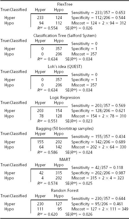
We once thought that the impact of our SNP genotypes, if they bear on hypertensive status, should predispose Chinese and Japanese women in the same ways. We have described difficulties with the SAPPHIRe sampling scheme already. Recruitment in Taiwan focused far more on hypotensive sibs of hypertensive probands than did recruitment in Hawaii. The majority of our Chinese women were from Taiwan and the majority of Japanese women were from Hawaii. No matter the “true” fractions of hyper and hypo within families in the two groups, the prevalence of hypertensives in our sample was far higher for the Japanese than for the Chinese. There are in total 161 samples, 23 hypotensive and 138 hypertensive, which is unlikely to be the distribution in the general population. Moreover, classifying with the same products of priors and misclassification costs (2:1 in favor of hypotensives in the Chinese) produced nothing of interest in the smaller Japanese group. When the ratio was changed to 6:1, a story emerged. The final tree has two splits. The classification was reasonably good, with cross-validation showing 30 misclassified among 161. Given that the Japanese were older than the Chinese, it is not surprising that by and large, the SNPs that figure in our two-split tree are nearly all SNPs that figure in the split of postmenopausal Chinese women. As one might expect, age did not figure in either split for the Japanese. As with the Chinese, there was a wide difference between significance as judged by Hotelling's T² and by bootstrap/permutation χ², implying that any impact of genes is additive. For details see Supporting Elaboration.

References

- 1.Breiman, L., Friedman, J. H., Olshen, R. A. & Stone, C. J. (1984) Classification and Regression Trees (Wadsworth, Belmont, CA), 1st Ed.
- 2.Zhang, H. (1998) J. Am. Stat. Assoc. 93, 180–193. [Google Scholar]
- 3.Zhang, H. & Bonney, G. (2000) Genet. Epidemiol. 19, 323–332. [DOI] [PubMed] [Google Scholar]
- 4.Tibshirani, R., Hastie, T. & Buja, A. (1995) Ann. Stat. 23, 73–102. [Google Scholar]
- 5.Hastie, T., Friedman, J. H. & Tibshirani, R. (2001) The Elements of Statistical Learning: Data Mining, Inference and Prediction (Springer, New York), 1st Ed.
- 6.Hastie, T., Tibshirani, R., Eisen, M., Brown, P., Ross, D., Scherf, U., Weinstein, J., Alizadeh, A., Staudt, L. & Botstein, D. (August 4, 2000) Genome Biol. 1, 10.1186/gb-2000-1-2-research0003. [DOI] [PMC free article] [PubMed]
- 7.Lynch, M. & Walsh, B. (1998) Genetics and Analysis of Quantitative Traits (Sinauer, Sunderland, MA).
- 8.Loh, W. Y. & Vanichsetakul, N. (1988) J. Am. Stat. Assoc. 83, 715–724. [Google Scholar]
- 9.Loh, W. Y. & Shih, Y. S. (1997) Statistica Sinica 7, 815–840. [Google Scholar]
- 10.Ruczinski, I., Kooperberg, C., Leblanc, M. (2003) J. Comput. Graph. Stat. 12, 475–511. [Google Scholar]
- 11.Breiman, L. (2001) Mach. Learn. 45, 5–32. [Google Scholar]
- 12.Lifton, R. P. (1996) Science 272, 676–680. [DOI] [PubMed] [Google Scholar]
- 13.Lifton, R. P., Dluhy, R. G., Rich, G. M., Cook, S., Ulick, S. & Lalouel, J. M. (1992) Nature 355, 262–265. [DOI] [PubMed] [Google Scholar]
- 14.Chuang, L. M., Hsiung, C. A., Chen, Y. D., Ho, L. T., Sheu, W. H., Pei, D., Nakatsuka, C. H., Cox, D., Pratt, R. E., Lei, H. H. & Tai, T. Y. (2001) J. Mol. Med. 79, 656–664. [DOI] [PubMed] [Google Scholar]
- 15.Reaven, G. M. (2003) Curr. Atheroscler. Rep. 5, 364–371. [DOI] [PubMed] [Google Scholar]
- 16.Lin, A., Lenert, L. A., Hlatky, M. A., McDonald, K. M., Olshen, R. A. & Hornberger, J. (1999) Health Serv. Res. 34, 1033–1045. [PMC free article] [PubMed] [Google Scholar]
- 17.Bechtel, S., Belkina, N. & Bernhardt, R. (2002) Eur. J. Biochem. 269, 1118–1127. [DOI] [PubMed] [Google Scholar]
- 18.Elchebly, M., Payette, P., Michaliszyn, E., Cromlish, W., Collins, S., Loy, A. L., Normandin, D., Cheng, A., Himms-Hagen, J., Chan, C. C., et al. (1999) Science 283, 1544–1548. [DOI] [PubMed] [Google Scholar]
- 19.Ostenson, C. G., Sandberg-Nordqvist, A. C., Chen, J., Hallbrink, M., Rotin, D., Langel, U. & Efendic, S. (2002) Biochem. Biophys. Res. Commun. 291, 945–950. [DOI] [PubMed] [Google Scholar]
- 20.Wu., X., Hardy, V. E., Joseph, J. L., Jabbour, S., Mahadev, K., Zhu, L. & Goldstein, B. J. (2003) Metabolism 52, 705–712. [DOI] [PubMed] [Google Scholar]
- 21.Bonnardeaux, A., Davies, E., Jeunemaitre, X., Fery, I., Charru, A., Clauser, E., Tiret, L., Cambien, F., Corvol, P. & Soubrier, F. (1994) Hypertension 24, 63–69. [DOI] [PubMed] [Google Scholar]
- 22.Morello, J. P. & Bichet, D. G. (2001) Annu. Rev. Physiol. 63, 607–630. [DOI] [PubMed] [Google Scholar]
- 23.Ranade, K., Wu, K. D., Hwu, C. M., Ting, C. T., Pei, D., Pesich, R., Hebert, J., Chen, Y. D., Pratt, R., Olshen, R. A., et al. (2001) Hum. Mol. Genet. 10, 2157–2164. [DOI] [PubMed] [Google Scholar]
- 24.Friedman, J. H., Hastie, T. & Tibshirani, R. (2000) Ann. Stat. 28, 307–337. [Google Scholar]
- 25.Breiman, L. (1996) Mach. Learn. 26, 123–140. [Google Scholar]
Associated Data
This section collects any data citations, data availability statements, or supplementary materials included in this article.