Selective 2′-hydroxyl acylation analyzed by primer extension and mutational profiling (SHAPE-MaP) for direct, versatile, and accurate RNA structure analysis

Abstract

SHAPE chemistries exploit small electrophilic reagents that react with the 2′-hydroxyl group to interrogate RNA structure at single-nucleotide resolution. Mutational profiling (MaP) identifies modified residues based on the ability of reverse transcriptase to misread a SHAPE-modified nucleotide and then counting the resulting mutations by massively parallel sequencing. The SHAPE-MaP approach measures the structure of large and transcriptome-wide systems as accurately as for simple model RNAs. This protocol describes the experimental steps, implemented over three days, required to perform SHAPE probing and construct multiplexed SHAPE-MaP libraries suitable for deep sequencing. These steps include RNA folding and SHAPE structure probing, mutational profiling by reverse transcription, library construction, and sequencing. Automated processing of MaP sequencing data is accomplished using two software packages. ShapeMapper converts raw sequencing files into mutational profiles, creates SHAPE reactivity plots, and provides useful troubleshooting information, often within an hour. SuperFold uses these data to model RNA secondary structures, identify regions with well-defined structures, and visualize probable and alternative helices, often in under a day. We illustrate these algorithms with the E. coli thiamine pyrophosphate riboswitch, E. coli 16S rRNA, and HIV-1 genomic RNAs. SHAPE-MaP can be used to make nucleotide-resolution biophysical measurements of individual RNA motifs, rare components of complex RNA ensembles, and entire transcriptomes. The straightforward MaP strategy greatly expands the number, length, and complexity of analyzable RNA structures.

INTRODUCTION

RNA plays many fundamental biological roles, often by interacting with other RNAs, proteins, and small molecules^1–3. In these roles, RNA molecules must adopt specific secondary and tertiary structures, the details of which are often difficult or impossible to characterize from sequence alone. A wide variety of chemical probing approaches have proven to be powerful tools for understanding the critical features of RNA structure at both small and large scales^4–6. Of these, SHAPE (selective 2′-hydroxyl acylation analyzed by primer extension) has emerged as a particularly useful probe of RNA structure. SHAPE uses small hydroxyl-selective electrophilic reagents to probe the reactivity of the RNA ribose 2′-OH group. SHAPE reactivities are insensitive to base identity and correlate with local nucleotide flexibility and dynamics^7–9 because flexible residues sample a wide range of conformations, a subset of which enhance the reactivity of the 2′-hydroxyl¹⁰ (Fig. 1a).

Figure 1.

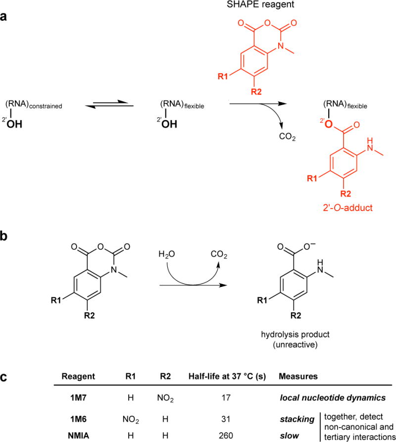
SHAPE chemistry and useful SHAPE reagents. (a) SHAPE reagents react preferentially with the 2′-hydroxyl groups of conformationally flexible RNA nucleotides⁷. (b) Quenching of SHAPE reagents via hydrolysis. (c) Overview of the three most useful SHAPE reagents. 1M7 is the workhorse SHAPE reagent; its reactivity with RNA measures local nucleotide flexibility^7,8,18 1M6 and NMIA are selective for nucleobases that have one face available for stacking and that achieve a reaction-competent conformation on a slow timescale, respectively. Together, 1M6 and NMIA can be used to detect non-canonical and tertiary interactions in RNA⁵³ and to increase the accuracy of secondary structure modeling²¹.

SHAPE chemistry makes it possible to thoroughly examine RNA structure because, with the exception of some post-transcriptionally modified RNAs, all RNA nucleotides carry a 2′-hydroxyl group. SHAPE reactions are self-inactivating through a competing hydrolysis reaction with water (Fig. 1b) and thus require no specific quench step. Because few compounds have a net reactivity as high as 55 M water, intrinsic SHAPE reactivities are largely insensitive to the presence of (additional) competing small molecules, ligands, and proteins. SHAPE experiments work robustly when performed in complex environments including those inside virus particles^11–13 and in living cells^14–17. By careful choice of SHAPE reagent (Fig. 1c)^15,16,18 and experimental design, nucleotide flexibilities can be compared under different experimental or environmental conditions including cell-free versus in-cell and as a function of ligand and protein binding. When used as constraints in RNA modeling algorithms, SHAPE reactivity data yield accurate secondary structure models for many classes of RNA^19–21.

Development of SHAPE-MaP, ShapeMapper and SuperFold

SHAPE and other RNA structure-probing approaches have recently been combined with massively parallel sequencing to enable the study of larger and more complex RNA systems^6,22–27. These approaches have used similar adapter-ligation methods and suffer from common limitations arising from multi-step library preparation protocols and low signal levels (see Alternative Methods below). To overcome these limitations we developed SHAPE-MaP, a direct, rapid and robust strategy for RNA structure probing at multiple scales.

SHAPE-MaP and ShapeMapper

In SHAPE-MaP, SHAPE adducts are detected by mutational profiling (MaP), which exploits an ability of reverse transcriptase enzymes to incorporate non-complementary nucleotides or create deletions at the sites of SHAPE chemical adducts (Fig. 2)²⁸. The ability of reverse transcriptase to occasionally extend through chemical lesions in RNA has been noted previously^29,30. Due to the optimized primer extension conditions used in the MaP approach, at least 50% of chemical adducts are detected²⁸. The cDNA generated are subjected to massively parallel sequencing, and mutations are counted to create SHAPE reactivity profiles using ShapeMapper (Fig. 2).

Figure 2.

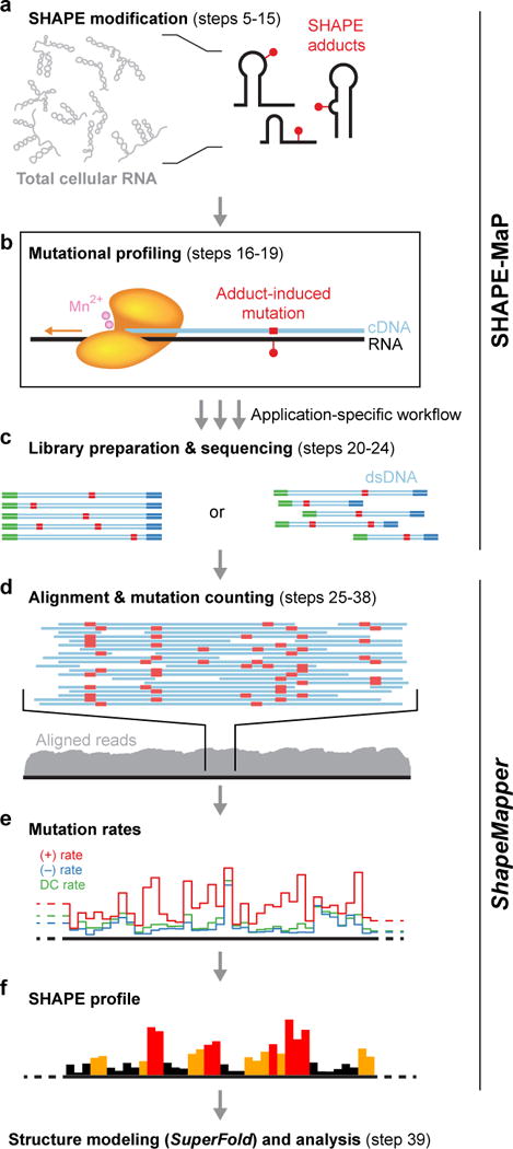
Overview of SHAPE-MaP and ShapeMapper. (a) RNA is treated with a SHAPE reagent that reacts at conformationally dynamic nucleotides. (b) Specialized reverse transcription conditions – the MaP strategy – allow the polymerase to read through chemical adducts in the RNA and to record the site as a nucleotide non-complementary to the original sequence in the cDNA. (c) The resulting cDNA is processed through one of three workflows (Fig. 4) and subjected to massively parallel sequencing. ShapeMapper then (d) aligns sequenced reads back to the target sequence, (e) calculates mutation rates, and (f) generates SHAPE reactivity profiles. SHAPE reactivities can be used to model secondary structures, visualize competing and alternative structures, and quantify any process that modulates local nucleotide RNA dynamics.

Because MaP sequencing data are digital and because both chemical modification and (no-reagent) non-modification are recorded for every nucleotide, analysis yields mutation frequencies. This enables two important advances over prior analog and other sequencing approaches. First, the signal requires no heuristic rescaling prior to background removal. Second, the standard error (a measurement of variability) associated with each SHAPE reactivity can be computed²⁸. These standard errors are conveniently viewed as error bars on reactivity profile plots, automatically produced by ShapeMapper.

Mismatches comprise about 60% of the sequence mutation signal detected by SHAPE-MaP; deletions make up the other 40%. Many deletions cannot be located unambiguously with single-nucleotide accuracy, especially in regions of repeated or homopolymeric sequence. For typical RNAs, approximately 55% of detected deletions (22% of total mutations) align ambiguously. ShapeMapper automatically detects ambiguously aligned deletions (Fig. S1) and excludes them from analysis to yield better agreement between SHAPE-MaP and previously validated SHAPE experiments (Fig. S2).

All current information supports the view that the MaP approach recovers chemical probing data equally as well as prior gold standard capillary electrophoresis methods. The MaP approach was intensively validated using a test set of RNAs ranging in size from 75 to 3,000 nucleotides²⁸.

SHAPE-MaP has been recently used to analyze the entire HIV-1 and hepatitis C virus (HCV) RNA genomes (~9,200 and 9,650 nts)^28,31,32. The new models for these two RNAs recapitulate nearly all previously known and accepted functional motifs and, moreover, contain multiple new structural and functional elements including experimentally validated pseudoknots²⁸ and other structures^31,32.

SuperFold algorithm

We recently developed a folding pipeline for modeling large RNAs²⁸. This pipeline, now called SuperFold, is fully automated (Fig. 3). SuperFold takes a windowing approach to folding of large RNAs. For long RNAs, practical window size choices are roughly 1,200 nucleotides for a partition function calculation and 3,000 nucleotides for a minimum free energy calculation. Dividing the folding of a large RNA into smaller segments allows modern multi-core workstations to model RNA structures in a modest amount of clock-time. SuperFold runs in three main stages (Table 4): partition function calculation, minimum free energy calculation, and structural analysis (Fig. 3). The partition function and minimum free energy structure calculation are implemented using RNAstructure³³, which enables direct incorporation of SHAPE reactivity information^19–21.

Figure 3.

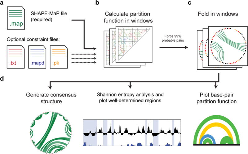
Overview of the SuperFold pipeline. (a) User-defined input files. Only the “.map” file is required. Optional files allow for modeling of tertiary interactions and pseudoknots, and inclusion of differential SHAPE reactivities²¹ in the energy function. (b) Partition function calculation. Calculations are performed using overlapping 1,400-nt windows; positions within 300 nucleotides of window end sites are not used in the calculation. The partition function for the full-length RNA is the average across each window in which a given base pair is able to occur. (c) Windowed folding. Base pairs with 99% probability are used as pairing constraints in a minimum free energy calculation in windows of 4,000 nts. (d) Structure visualization. A consensus structure is generated by requiring that base pairs identified during windowed folding (step c) occur in greater than one-half of windows. A Shannon entropy analysis is used to identify well-determined regions, and the partition functions of probable base pairs are plotted as arcs across the RNA.

Table 4. SuperFold stages and output files.

The initialization stage is executed by the user using the Superfold.py executable. RNAtools.py contains companion classes used by SuperFold. Output directories are named after the input .map file and appended with a hash of the input flags, allowing the user to run multiple jobs within the same directory without encountering conflicting file names. All command line parameters are stored in the log file within the results directory.

Stage	Script/executable	Output files/directories
Initialization	Superfold.py RNAtools.py	results_RNAname_hash/: A results directory with the name of the .map file and a cryptographic hash. All results files will be placed in this directory. log_result*.txt: log file detailing the status of the run.
Partition function calculation	partition (RNAstructure) ProbabilityPlot (RNAstructure) batchSubmit.py	Partition_RNAname_hash/: intermediate files from the windowed partition function calculation will be placed here.
Minimum free-energy (MFE) calculation	Fold (RNAstructure) batchSubmit.py	fold_RNAname_hash/: intermediate files from the MFE calculation will be placed here.
Figure drawing	pvclient.py PyCircleCompare.py drawArcRibbons_simple.py	Analysis files are placed in the results folder: Shannon entropy/SHAPE analysis, partition function arcs, and circle plots and secondary structure diagrams of Shannon entropy/SHAPE regions. Text files for use in a plotting program are also created here.

Two assumptions are made to model RNA folding in windows. The first is that RNA structure is predominately local in nature. A maximum pairing distance of 600 nts is currently implemented in RNAstructure. It is a practical, but imperfect, assumption that pairing does not occur outside this number of nucleotides^19,21. A consequence of this implementation is that improperly choosing the “ends” of an RNA will introduce (potentially) cascading effects on nucleotide pairing. To mitigate this effect, predicted structures 300 nucleotides from the 5′ and 3′ ends of a given window are removed. The second assumption is that the most stable structure will predominate despite potentially poorly chosen 5′ and 3′ ends. SuperFold combines predicted pairs from overlapping windows and requires that base pairs occur in more than half of potential cases to be retained in a minimum free energy secondary structure model.

The partition function computed over a given RNA can be used to distinguish regions of an RNA that form well-defined structures from those that are likely to exist as an ensemble of structures³⁴. SuperFold calculates the partition function in windows of 1200 nucleotides. Interactions within 300 nucleotides of the window 5′ and 3′ ends are removed. Pairing probabilities are then averaged across each window in which a given base pair is able to occur. Additional partition function calculations are performed using the true 5′ and 3′ ends to reduce de-weighting of the partition function at the ends of an RNA.

The partition function can also be used to identify helices that are most likely to be modeled correctly. Nucleotides with predicted pairing probabilities above 0.99 appear to be correct more than 90% of the time³⁵. This observation is used to constrain the minimum free energy structure prediction using RNAstructure Fold in 3,000-nt sliding windows. Highly probable pairs, based on the partition function within a folding window, are constrained to be base paired. Nucleotides split by an overlapping window are forced to be single stranded. The combination of these two constraints mitigates the effects of inadvertently poorly chosen ends.

Identifying well-determined RNA structures

From the partition function of base pairing, a SHAPE data-informed Shannon entropy³⁶ can be calculated. Analysis of the Shannon entropy of base pairing can be used to quantify the well-determinedness of an RNA conformation within a given region^28,35. Low SHAPE reactivity across a region of RNA is indicative of stable base pairing. Regions that have both low SHAPE reactivities and low Shannon entropy are likely to exist in a single structural state and have been found to be highly correlated with known functional RNA structures in both the HIV-1 and HCV RNA genomes^28,31. Regions are calculated as the median over 55-nt windows of Shannon entropy and SHAPE reactivity. Because these low Shannon entropy and SHAPE reactivity regions are calculated over (large) windows, base pairs may fall outside of strict boundaries. In SuperFold, these regions are discovered and then expanded to include nearby minimum free energy model helices that cross low SHAPE and low Shannon entropy boundaries to contain complete helical elements and to account for imprecise boundaries of well-determined regions.

Pseudoknots

The de novo discovery of RNA pseudoknots remains challenging. Several new pseudoknots were discovered in the HIV-1 RNA genome using a process that was not fully automated²⁸. We have obtained good results using the ShapeKnots algorithm²⁰ with 700-nt windows in 50-nt steps. Pseudoknots that appear in a majority of windows are set aside for further analysis by an expert user for plausibility. Additional experimental validation or evolutionary support should then be sought because, in practice, false positive predictions are obtained with arbitrarily chosen 5′ and 3′ window boundaries. Once a pseudoknot has been located, the pseudoknot can be readily flagged in SuperFold.

Overview of the Procedure

Here, we provide a detailed protocol for SHAPE-MaP and for subsequent data analysis using ShapeMapper and SuperFold. For simplicity, the Procedure focuses on a straightforward folding approach for interrogating native-like or deproteinized RNA with 1-methyl-7-nitroisatoic anhydride (1M7). Adapting the Procedure for other RNAs, for in-cell conditions, and for other SHAPE reagents is discussed in Experimental Design. The key stages of the Procedure are as follows:

SHAPE modification of RNA

SHAPE electrophiles are added to the folded RNA (or virus or cell) and then incubated until the reagent has either reacted with RNA or degraded via hydrolysis with water (5 hydrolysis half-lives, Figs. 1b, c). Two control reactions are performed in parallel: a no-reagent control and a denaturing control. In the no-reagent control reaction, folded RNA is incubated with solvent only (typically DMSO for SHAPE reagents); this important control measures the intrinsic background mutation rate of reverse transcriptase under MaP conditions and also detects certain naturally occurring RNA modification events. In the denaturing control reaction, RNA is suspended in a denaturing buffer containing formamide and incubated at 95 °C prior to modification with SHAPE reagent. Nucleotides are modified relatively evenly in this step, and the resulting site-specific mutation rates account for subtle sequence- and structure-specific biases in detection of adduct-induced mutations. Thus, a complete SHAPE-MaP experiment consists of three reactions: plus-reagent (+), minus-reagent (−), and denaturing control (DC).

The tagmentation (Nextera) library preparation used in this protocol requires that only double-stranded DNA (dsDNA), derived from the RNA that is being structurally interrogated, be present in the sample. It is thus critical that genomic DNA and template DNA from cellular and in vitro-transcribed samples, respectively, be completely removed prior to reverse transcription and subsequent library preparation steps. Cellular or viral RNAs that were obtained by gentle extraction to maintain secondary structure should be DNase-treated following SHAPE modification, prior to reverse transcription. For in vitro-transcribed RNAs, a DNase treatment is conveniently performed immediately following in vitro transcription.

Mutational Profiling (MaP) by reverse transcription

After SHAPE modification of RNA, reverse transcriptase is used to create a mutational profile (MaP). This step encodes the positions and relative frequencies of SHAPE adducts as mutations in the cDNA sequence. Mutational profiling is efficient, with roughly 50% of SHAPE adducts detected as mutations in the cDNA²⁸. The reverse transcription reaction conditions are the same for any RNA, but the researcher has two options for DNA primer type. RNAs that are small enough to be sequenced end-to-end in a single massively parallel sequencing read (read lengths up to 600 nts are currently possible) can be subjected to reverse transcription with standard sequence-specific DNA primers. Specific primers can also be used to probe a specific sub-region of a large RNA (Fig. 4, Small RNA and Amplicon Workflows). Use of gene- or region-specific primers also makes it possible to analyze a specific, rare RNA in a complex mixture of RNAs. This is especially useful for in-cell studies. For analysis of large RNAs, the constituents of entire transcriptomes or of multi-component ribonucleoprotein or long noncoding RNA assemblies, random primers facilitate even coverage of complex RNA states in a single experiment (Fig. 4, Randomer Workflow). Following mutational profiling with appropriate primers, one of these three workflows (Fig. 4) is then used for library construction.

Figure 4.

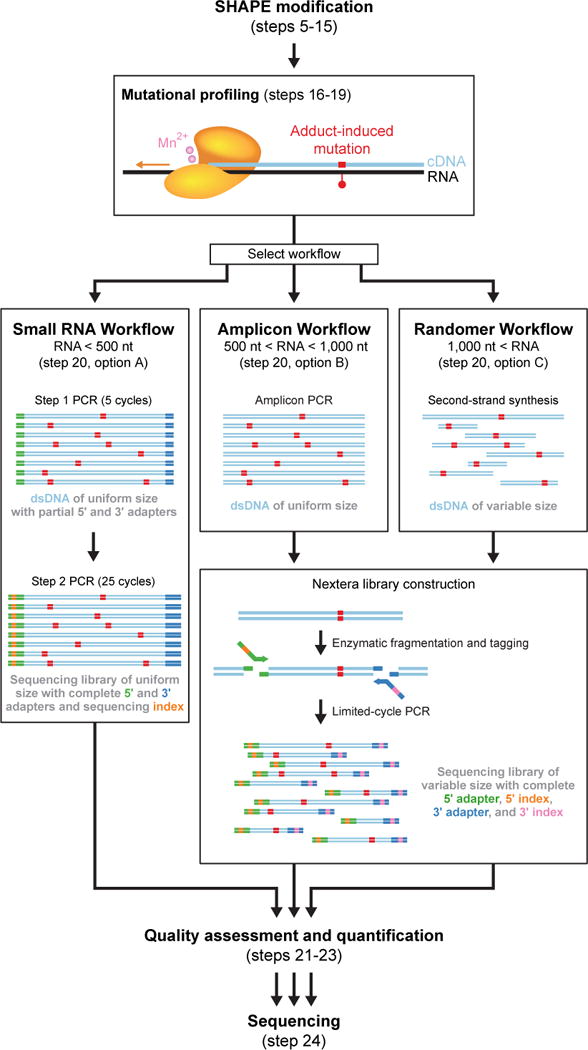
Overview of workflows useful for converting RNAs modified with SHAPE reagents into libraries compatible with massively parallel sequencing. RNAs are modified with a SHAPE reagent and subjected to reverse transcription under MaP conditions, during which adduct-induced mutations are recorded in the cDNA strand. One of three workflows is then used to construct high-quality libraries for sequencing and recovery of the SHAPE chemical probing information.

Library construction and sequencing

The Small RNA Workflow is ideally suited for short RNAs or sub-regions of large RNAs that are sufficiently short to be completely sequenced by a single unpaired sequencing read or by two mated paired-end sequencing reads. Libraries prepared with this workflow reflect the strandedness of the original RNA. After reverse transcription with sequence-specific primers, purified cDNA is “tagged” with incomplete platform-specific adapters in a limited-cycle PCR reaction. The resulting dsDNA product is purified and further amplified in a second PCR reaction that completes the platform-specific adapters and adds sequences necessary for multiplexing (see Reagent Setup). After purification, sequencing libraries are of uniform size and each DNA molecule contains the entire sequence of interest (Fig. 6a).

Figure 6.

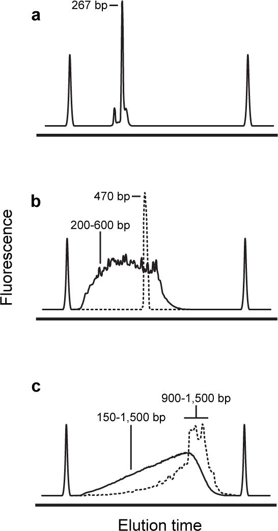
Representative library size distributions as a function of workflow. (a) Bioanalyzer electropherogram of a TPP riboswitch library produced with the Small RNA Workflow. The small peak to the left of the major product is unconverted Step 1 PCR product. (b) A library (solid line) constructed from a single amplicon (dashed line) via the Amplicon Workflow. The library contains some DNAs slightly larger than the original amplicon because platform-specific adaptors are added to near-full length fragments. (c) A library (solid line) constructed via the Randomer Workflow. The sizes of dsDNA produced by second-strand synthesis (dashed line) set the upper limit on the library size.

The Amplicon Workflow is well suited for large, low-abundance RNAs or for sub-regions of large RNAs that cannot be sequenced end-to-end by a single sequencing read. After reverse transcription, purified cDNA is amplified via PCR with sequence-specific primers. The resulting dsDNA is then enzymatically fragmented and tagged with platform-specific adaptors and multiplexing indices. Sequencing libraries constructed in this way are of variable size; each molecule contains a fragment of the original amplicon (Fig. 6b). Information regarding the strand of origin is lost with this method. Typically, when the Amplicon Workflow is used to construct a sequencing library, reverse transcription is primed with sequence-specific primers. However, if the researcher wishes to generate a sequencing library for a specific region of an RNA that was initially converted to cDNA using random primers, the Amplicon Workflow allows for targeted “re-construction” of libraries.

The Randomer Workflow can be used to construct sequencing libraries when the RNA of interest is large (greater than ~500 nt) and reasonably pure; for example, in the case of a viral RNA genome. The Randomer Workflow also is appropriate for analysis of very complex systems including complete RNA transcriptomes. Researchers who wish to examine RNAs for which sequence directionality is unknown should use alternate, strand-information preserving methods (not described in this protocol). After reverse transcription with appropriate random primers, purified cDNA is converted to dsDNA and then enzymatically fragmented and tagged with platform-specific adapters and multiplexing indices. The resulting sequencing library is of variable size, and each molecule corresponds to a fragment of the original RNA (Fig. 6c).

After construction of high-quality SHAPE-MaP libraries, the libraries are subjected to sequencing with a massively parallel sequencing instrument. This protocol describes preparation of libraries compatible with Illumina sequencing instruments. However, the MaP approach is fully compatible with any platform with a high per-nucleotide calling accuracy. To accurately recover nucleotide-resolution structural information, SHAPE-MaP requires high read depths across all regions of the RNA of interest.

For a given RNA, SHAPE-MaP involves generation of sequencing data for RNA treated under three distinct experimental conditions: plus-reagent, minus-reagent, and denaturing control. For input into ShapeMapper, these samples can either be sequenced separately or sequenced together and deconvoluted using multiplexed barcodes (such as Illumina TruSeq). Sequencing reads should be output as FASTQ files, a format widely available with modern sequencing platforms.

Hit level and read depth requirements

As discussed in the initial SHAPE-MaP publication and by other investigators^24,37, the physical accuracy of an RNA structure probing experiment is tightly coupled to both the observed signal above background and to sequencing read depth, issues often overlooked for approaches that link chemical probing and massively parallel sequencing. To consistently and accurately model RNA structures, we recommend a “hit level” (total background-corrected signal per transcript nucleotide) of about 5 or greater, corresponding to a per-nucleotide read depth of about 1,000–2,000 given current SHAPE adduct-induced mutation rates²⁸. This is substantially higher than the depths required to assess RNA expression levels, to perform ribosome profiling, or to enable genome assembly. In a SHAPE-MaP experiment, structure probing information is obtained for most nucleotides in a sequencing read. Given that sequencing reads of 100–600 or more nucleotides are now routine, these read-depth requirements are readily attainable using current technology. Multiple RNAs, each thousands of nucleotides long, can be sequenced at sufficient depth for accurate SHAPE-MaP structure modeling in a single run on a laboratory-scale instrument.

Generation of SHAPE profiles with ShapeMapper

ShapeMapper is designed to run to completion with no user intervention following the set-up step. A simple user-edited configuration file informs ShapeMapper which RNA sequences are present in each file and which sequences correspond to the three experimental conditions. The configuration files also defines several global run parameters (Box 1). ShapeMapper uses a single Python script executed by the user to begin analysis and then runs each analysis stage in series. Several analysis stages rely on third-party programs (see Supporting Protocol 1 and Table 3), the most important of which is the sequence alignment software Bowtie2³⁸, although any algorithm that supports gapped alignment could be substituted.

Box 1. Example ShapeMapper configuration file.

• ## ShapeMapper stages to run

• buildIndex = on

• trimReads = on

• alignReads = on

• parseAlignments = on

• countMutations = on

• pivotCSVs = on

• makeProfiles = on

• foldSeqs = off

• renderStructures = off

• ## Global run options. Only important parameters are shown.

• # trimReads options

• minPhred = 20

• windowSize = 1

• minLength = 25

• # alignment options

• maxInsertSize = 500

• # countMutations options

• randomlyPrimed = on

• primerLength = 10

• minMapQual = 30

• ## Specify which RNAs are present in each pair of FASTQ files.

• ## FASTQ file sample names on left, comma-separated alignment

• ## target sequence names on right.

• [alignments]

• 3 = 16S

• 2 = 16S, TPP_riboswitch

• 7 = 16S

• 1 = TPP_riboswitch

• 4 = TPP_riboswitch

• # Alternative syntax (specify full FASTQ # filenames)

• more_16S: additional_16S_rx_R1.fastq, additional_16S_rx_R2.fastq = 16S

• ## Specify which files correspond to the three experimental conditions

• ## (SHAPE-modified, untreated, and denatured control) and name each

• ## reactivity profile to be output.

• [profiles]

• name = TPP riboswitch

• target = TPP_riboswitch

• plus_reagent = 1

• minus_reagent = 2

• denat_control = 4

• name = Small subunit ribosome

• target = 16S

• plus_reagent = 3, more_16S

• minus_reagent = 2

• denat_control = 7

Table 3. ShapeMapper stages.

The initialization stage is directly executed by the user; all subsequent stages are launched automatically from the ShapeMapper.py script. “RUN” indicates the path to the folder from which ShapeMapper was executed, which should contain FASTA reference sequences, raw sequencing reads, and a configuration file. “conf” indicates configuration file parameters. “*” is a wildcard character indicating multiple names.

Stage	Script/executable name	Output files/directories
Initialization and configuration file; verification/loading	ShapeMapper.py, parseConfigFile.py, conf.py	RUN/log.txt: file that logs pipeline stage execution and error messages. RUN/temp: folder that stores subprocess standard out and standard error streams during execution (can be deleted after run completion). RUN/output: folder that will store the bulk of the pipeline output. RUN/output/*: subfolders that will store the output from each pipeline stage.
Quality trimming	trimPhred	RUN/output/trimmed_reads/*.fastq: sequencing reads trimmed left-to-right at the site of the first average phred score below conf.minPhred over a window of length conf.windowSize with resulting read lengths greater or equal to conf.minLength.
Sequence alignment preparation	bowtie2-build (third party)38	RUN/output/bowtie_index/*: Bowtie2 reference sequence indices.
Sequence alignment	bowtie2 (third party)38	RUN/output/aligned_reads/*.sam: aligned sequence files, one file for each line in configuration file section “[alignments]”.
Alignment parsing and ambiguously aligned deletion identification	parseAlignment	RUN/output/mutation_strings/*.txt: parsed and simplified alignments.
Mutation counting	countMutations, pivotCSV.py	RUN/output/counted_mutations/*.csv: mutation counts and read depths written to comma-separated files, one file for each line in configuration section “[alignments]”. RUN/output/counted_mutations_columns/*.csv: the same files arranged in column format. These files also contain the total mismatch count, total deletion count, and total unambiguously aligned deletion count.
Reactivity profile creation and standard error calculation	generateReactivityProfiles.py (uses matplotlib – third party)	RUN/output/reactivity_profiles/*.tab: the most detailed output, containing mutation rates, depths, reactivities, and standard errors in tab-delimited columns. RUN/output/reactivity_profiles/*.shape: simple SHAPE reactivity file, tab-delimited columns with nucleotide numbers in the first column and reactivities in the second, no-data positions indicated by −999. RUN/output/reactivity_profiles/*.map: SHAPE reactivity file including standard errors and nucleotide sequence. RUN/output/reactivity_profiles/*_histogr ams.pdf: histograms of mutation rates, read depths, and reactivities that are useful for troubleshooting. RUN/output/reactivity_profiles/*_depth_and_reactivity.pdf: read depth profile, mutation rate above background profile, and reactivity profile images.
Structure modeling	Fold (part of RNAstructure – third party)33	RUN/output/folds/*.seq: reference sequence files in the format required by RNAstructure. RUN/output/folds/*.ct: structure models, one file for each line in configuration file section “[folds]”.
Structure drawing	pvclient.py (custom client for the Pseudoviewer web service – third party)58	RUN/output/folds/*.eps: postscript image files for the lowest predicted free energy structure colored by SHAPE reactivity, for each RNA specified in configuration section “[folds]” RUN/output/folds/*.xrna: XRNA files for each lowest predicted free energy structure, which can be manually edited if desired.

For short RNAs with high-quality SHAPE data (small standard errors), SHAPE reactivities can be fed directly into RNAstructure³³ as soft constraints^19–21 for structure modeling. For larger RNAs, the windowed folding strategy implemented in SuperFold is required.

Applications of SHAPE-MaP

MaP allows RNAs of virtually any size to be analyzed in a single experiment, facilitates rapid multiplexed library preparation, and permits fully automated data analysis. The effects of sequence polymorphism and co-existing ribosnitches²⁸ can be evaluated and compared from single experiments provided the region under interrogation is completely sequenced in each read. The MaP experiment includes a DNA amplification step; therefore, RNAs present in scarce amounts or in complex mixtures can be examined. The MaP approach even enables probing of synthetic genetic polymers (XNAs), nucleic acid-like molecules with backbone chemistries not found in nature³⁹. In sum, any RNA that can be amplified by RT-PCR should be amenable to single-nucleotide resolution SHAPE-MaP analysis.

SHAPE-MaP reactivity information can be used in numerous informative ways. For large-scale RNA structure analysis, three applications are especially useful. First, SHAPE reactivities, coupled with an estimate of how often regions form unique versus competing folds, can be used to identify regions that are likely structured^28,31. These highly structured regions appear to correlate strongly with functional motifs. Second, SHAPE reactivity data can be incorporated as a pseudo-free energy change term for RNA secondary structure modeling. In extensive validation experiments, this approach recovers 90% or more of accepted base pairs in well-characterized RNAs^21,28. Third, SHAPE reactivity data are ideal for visualizing changes in RNA structure as a function of diverse biological processes such as ligand binding^40,41, RNA folding and assembly^42–44, and interaction with proteins^11,12,44, and for evaluating the complex effects of the cellular environment^15–17. SHAPE-MaP experiments efficiently generate RNA chemical probing data across many thousands of nucleotides.

Alternative methods

There has recently been intense interest in linking RNA structure probing with readout by massively parallel sequencing^22–27 and the reagents employed for structure probing have been extensively reviewed^4,6. The MaP strategy is unique because the site of chemical modification is recorded internal to the sequenced region. In other strategies, reverse transcription is blocked by the base modification and thus the terminus of the sequenced fragment corresponds to a site of chemical modification in the targeted RNA. These adduct-terminated fragments are then prepared for massively parallel sequencing using approaches based on construction of conventional RNA-seq libraries. These methods all measure RNA modifications using single-stranded adaptor ligation, which is strongly influenced both by local sequence and structural effects and by many post-ligation library preparation steps⁴⁵. In our laboratory, we found that two distinct approaches employing single-stranded adaptor ligation failed to maintain the quantitative relationship between SHAPE probing and underlying RNA structure⁴⁶. In addition, many early methods used chemical or enzyme reagents that react with and report on only a subset of the four major RNA nucleotides. These data lead to notable blank spots in RNA structural information, and it is not known how to use such data to model large RNA structures with high accuracy.

In the MaP strategy, the reverse transcriptase enzyme reads through the sites of chemical adducts in an RNA: it does not matter where the cDNA begins or ends. MaP experiments therefore appear to be substantially impervious to the substantial sequence- and structure-based biases introduced during construction of the libraries required for massively parallel sequencing. The MaP approach is also insensitive to single-strand breaks and background degradation and does not exhibit signal decay or drop-off with long cDNA products²⁸, effects that result in significant noise for alternative sequencing-based strategies for detecting chemical modification of RNA.

The ability to recover RNA structure information accurately has the direct consequence that SHAPE-MaP reactivities make possible RNA secondary structure modeling using well-established and validated parameters^20,21. Based on analysis of a test set of small and large RNAs, SHAPE-directed secondary structure modeling recovers accepted base pairs with an overall sensitivity of 92% and a positive predictive value of 86%²⁸. Structure probing approaches based on single-stranded adaptor ligation have met with limited success in data-driven structure modeling. Most reports have not examined structure modeling accuracy^{22,23,25,26,37}, have reported low accuracies^24,27,37, or have focused on short RNAs⁴⁷.

Advantages and limitations

MaP is a robust biochemical strategy for the quantification of extent of chemical adducts at individual nucleotides in nucleic acids^28,31,39,48. SHAPE-MaP equips any lab able to sequence DNA with the ability to probe nucleic acid structure at large scales and with nucleotide-resolution accuracy. Extensive validation experiments indicate that MaP enables nucleic acid probing experiments, read out by massively parallel sequencing, to reveal the underlying RNA structural information at the same high level of quantitative accuracy as prior highly labor-intensive approaches.

There are two fundamental physical requirements for successful SHAPE-MaP RNA structure interrogation. First, the RNA must be long enough to allow primer binding for reverse transcription. RNAs smaller than about 150 nucleotides are inefficiently recovered by the Randomer Workflow, and native (not in-vitro transcribed) RNAs smaller than about 40 nucleotides are difficult to study even using the Small RNA Workflow. Second, there must be a sufficient number of RNA molecules in the sample to accurately measure chemical adduct-induced mutation rates. Exceptionally rare transcripts or structures may simply not produce sufficient signal to be accurately distinguished from background noise.

ShapeMapper enables the rapid, automated analysis of data from MaP experiments using current-generation massively parallel sequencing instruments. A typical MiSeq experiment can be analyzed in less than an hour. ShapeMapper is optimized for analyzing lab-scale MaP experiments (total FASTQ file size under about 40 Gb). Larger datasets should be run in batches.

The RNA structure modeling rules implemented in SuperFold have been benchmarked against experimentally validated large RNAs with well-defined secondary structures, primarily the structures of ribosomal RNAs²⁸. The validations we have performed have been the most ambitious undertaken by any group to date. Although rRNAs make up a substantial fraction of the total mass of RNA in a cell, these RNAs may have overall structural features that are distinct compared to the diverse mRNAs, small RNAs, non-coding RNAs, and long non-coding RNAs that are also present in cells. Additionally, there are many functionally essential pairing interactions that are known to occur over thousands of nucleotides, outside the limits of current practical computational analysis^21,49.

Experimental design

Controls

Researchers new to RNA structure probing experiments may wish to include a positive control RNA in their experiments. We suggest using one of many well-structured RNAs that fold robustly and have been previously examined with SHAPE-MaP²⁸. This control can be spiked into samples, as long as it does not interact with the experimental RNA of interest.

RNAs and RNA folding

SHAPE-MaP may be applied to RNAs of any length or complexity; however, since SHAPE inherently probes the ensemble of RNA molecules present in the system of interest, conditions should be selected to ensure that the RNA sample is folded in a biologically relevant and informative state prior to probing. Depending on the experimental aims, researchers may choose to probe RNA transcripts synthesized in vitro, native transcripts gently isolated from cells or virions, entire transcriptomes in living cells, or a combination of these. Small, well-structured RNAs (for example, riboswitches and ribozymes) are generally amenable to in vitro transcription and refolding, while probing of large RNAs such as ribosomes should be performed using RNA extracted from cells under native-like conditions to preserve secondary and tertiary structure. Conditions for refolding many (but not all) in vitro-transcribed RNAs^7,50,51 and for extraction and purification of large, complex RNAs from virions and cells under non-denaturing conditions have been described^{11–13,19,52} and will not be extensively detailed here. Generally, when extracting RNA from cells or virions,, the use of denaturants, divalent ion chelators, and elevated temperature should be avoided. Direct interrogation of RNA structure inside cells by SHAPE works well^14–17. The protocol described here emphasizes simple folding procedures for interrogating relatively simple, in vitro-transcribed RNAs, but any procedure that folds an RNA into an informative state can be used, provided the pH is in the 7.4–8.3 range.

SHAPE probing reagents

In this protocol, we emphasize the use of 1-methyl-7-nitroisatoic anhydride (1M7)¹⁸, which is well validated for RNA structure analysis and modeling. Essentially identical approaches can be used with reagents 1-methyl-6-nitroisatoic anhydride and N-methyl-isatoic anhydride (1M6 and NMIA, respectively; Fig. 1c), and other reagents including DMS⁴⁸. Reactions with 1M6 are selective for nucleotides in which one face of the nucleobase is available for stacking. NMIA is used to identify nucleotides that are undergoing relatively slow conformational changes. These reagent-specific reactivities can be used both to identify residues that participate in non-canonical interactions and to improve RNA secondary structure modeling^21,53. In addition, the MaP strategy can be used to follow time-resolved RNA processes, in 1-sec snapshots, using the benzoyl cyanide (BzCN) reagent^42,54,55. The modest solubility and rapid hydrolysis of these reagents make over-modification of RNA samples virtually impossible.

In-cell analysis

No significant changes are required to execute this protocol following in-cell SHAPE probing and extraction of total cellular RNA by standard methods. Although Spitale et al. suggested that well-validated SHAPE reagents (Fig. 1) are not suitable for in-cell studies¹⁴, our extensive experience indicates that these SHAPE reagents work well in bacterial cells^15–17 and in multiple mammalian cell lines, including human lymphoblastoid, human liver, and mouse stem cells (L. Lackey, A. Laederach, D.M. Mauger, M.J.S. and K.M.W., unpublished). For precise details regarding in-cell SHAPE probing, we refer interested researchers to the cited publications and provide a brief overview here. SHAPE reagents (including 1M7) enter cells readily and without need for permeabilization. It is critical to ensure rapid, thorough mixing of the SHAPE reagent. For suspension cultures, simply adding a larger volume of cells to a smaller volume of SHAPE reagent is sufficient. Adherent cells are modified by adding SHAPE reagent directly to cells in fresh growth media, followed by swirling the tissue culture plate or flask to allow thorough mixing. The pH should be maintained in the 7.4–8.3 range. The recommended final concentration of SHAPE reagent is 10 mM.

There are critical experimental and biophysical advantages to using the fast-reacting and extensively validated 1M7 SHAPE reagent for in-cell RNA structure probing. First, 1M7 reacts over a period of roughly 2 minutes before being consumed by hydrolysis^15,18. This time frame nicely balances experimental ease of use with a biologically relevant time scale. Second, because 1M7 auto-inactivates within a few minutes, it is not necessary to add potentially harsh quenching agents. This feature allows intact RNA and RNA-protein complexes to be recovered from cells¹⁷. Third, 1M7 is relatively insensitive to trivial and non-biological features of a solution like divalent ion concentrations¹⁸. This means that, using 1M7, SHAPE reactivities for in-cell versus extracted or cell-free RNAs can be compared directly^15–17, as can experiments performed in virus particles or in crystals, which is not true for slower reacting reagents. Finally, because 1M7 is well-validated for SHAPE-directed secondary structure modeling, this reagent also makes it possible to model novel RNA structures in vivo^16,17,31.

Random priming

Conventionally, random hexamers have been used to prime cDNA synthesis; however, these primers lead to wildly unbalanced sequencing coverage of RNAs that is exacerbated in RNAs with a low fraction or uneven distribution of G and C nucleotides. To resolve this challenge, we use randomized 9-mer primers (Fig. 5)²⁸. These primers perform better than shorter random primers for all RNAs we have evaluated. For sequences in which GC content is low or unevenly distributed, we use “LNA+” primers²⁸. These primers omit cytosine to disfavor guanosine binding, contain 2,6-diaminopurine to favor binding to uracil, and include locked nucleic acid monomers (Fig. 5) to increase affinity. We recommend using LNA+ primers when the median GC count of 15-nt sliding windows along the length of the RNA sequence of interest is less than seven; otherwise, we recommend the use of randomized 9-mer primers.

Figure 5.

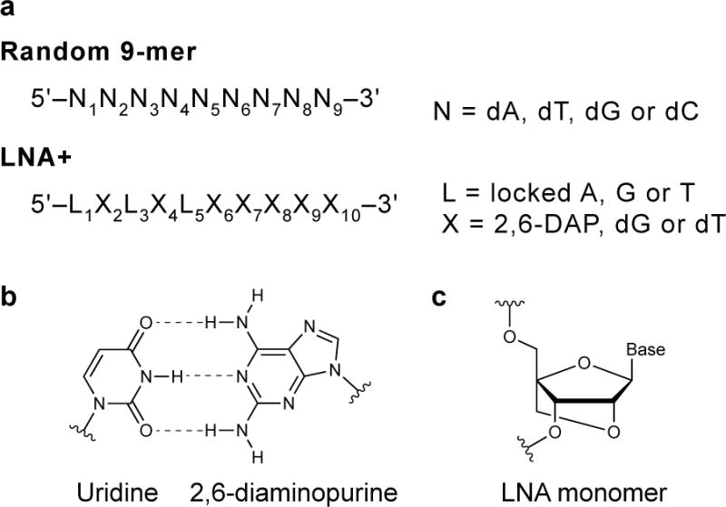
Random primer design. Nonamers used for randomly-primed reverse transcription. LNA+ primers are recommended for RNAs with high or uneven GC content. Uridine and 2,6-diaminopurine (DAP) nucleotides form three hydrogen bonds that increase primer affinity for target RNA. Locked nucleic acids also increase the stability of primer-RNA duplexes.

SuperFold options and advanced features

Several options can be used to modify SuperFold operation (Box 2). A full explanation of command line options is available in the README file. For example, the number of processors available to SuperFold should be set using the flag “—np”. This number is typically four or more on a desktop workstation.

Box 2. Command line flags to modify how SuperFold runs individual stages.

Flag [input]	Description
–help	Displays available flags with descriptions.
–ssRegion [.txt file]	Forces nucleotides in the user-supplied file SSREGION to be single stranded. See SuperFold readme for file format description.
–pkRegion [.txt file]	Models structure around pseudoknotted base pairs in the supplied PKREGION file. See SuperFold readme for file format description.
–np [int]	Sets the number of processors (NP) available to SuperFold. Default: 2.
–SHAPEslope [float]	SHAPE pseudo-free energy slope used for structure modeling. Value optimized in previous work19,20. Default: 1.8 kcal/mol.
–SHAPEintercept [float]	SHAPE pseudo-free energy slope used for structure modeling. Value optimized in previous work20. Default: – 0.6 kcal/mol.
–differentialFile [.txt file]	User-supplied differential SHAPE file calculated from NMIA-1M6. Refines ΔGSHAPE energy function21.
–differentialSlope [float]	Sets the pseudo free-energy slope for the differential SHAPE reactivity values. Default: 2.1 kcal/mol.
–trimInterior [int]	Number of nucleotides to trim from interior partition function and fold calculations. Default: 300.
–partitionWindowSize [int]	Length of the partition function window size. Default: 1200 nucleotides.
–partitionStepSize [int]	Spacing between partition function windows. Default: 100 nucleotides.
–foldWindowSize [int]	Length of the Fold window size. Default: 3000 nucleotides.
–foldStepSize [int]	Spacing between Fold windows. Default: 300 nucleotides.
–drawSS	Include secondary structure diagrams for expanded regions of low SHAPE and Shannon entropy using the Pseudoviewer58 web service.

Known pseudoknots can be included in the SuperFold structure prediction using a user-generated file, PKREGION, a tab-separated file with one nucleotide pair entered on each line. Nucleotide pairs included in this file will be forced to be single stranded during partition function and fold calculations. These pairs are added manually during the consensus structure generation step (Fig. 3). Similarly, nucleotides that are known to be single stranded (from complementary biological experiments) can be forced to be single stranded using a SSREGION file.

Use of a .map file alone means that RNA secondary structure modeling will be performed using the ΔG_SHAPE pseudo-free energy change term for reactivities based on the well-validated 1M7 SHAPE reagent. This approach generally yields high-quality secondary structure models^19,20. It is also possible (and recommended) to incorporate data from “differential”, or three-reagent, SHAPE experiments²¹ by incorporating the results of probing with 1M6 and NMIA, using a .mapd file.

MATERIALS

REAGENTS

A complete list of reagents necessary for all three workflows is listed below. Depending on the workflow, not all reagents are required.

RNA at a concentration of 5 μM in 10 mM HEPES, pH 8.0 CRITICAL: RNA must be prepared, stored, and manipulated in an RNase-free environment. For best results, reagents should be of highest possible quality and reserved for RNA use only. RNA can be stored at −20 °C for at least 6 months. Avoid repeated freeze-thaw cycles. The 5 μM concentration is convenient for in vitro studies; however, much lower concentrations of RNA can be probed using the Small RNA and Amplicon workflows.

• Sodium chloride (NaCl; 5 M, Life Technologies, cat. no. AM9760G)

• Magnesium chloride (MgCl₂; 1 M, Life Technologies, cat. no. AM9530G)

• Potassium chloride (KCl; 2 M, Life Technologies, cat. no. AM9640G)

• Tris, pH 8.0 (1 M, Life Technologies, cat. no. AM9850G)

• HEPES (Fisher Bioreagents, cat. no. BP310-500)

• EDTA, pH 8.0 (0.5 M, Life Technologies, cat. no. AM9260G)

• Formamide, highly deionized (Life Technologies, cat. no. 4311320)

• Manganese chloride (MnCl₂; 1 M, Fisher Bioreagents, cat. no. BP541-100)

DMSO, anhydrous (Sigma-Aldrich, cat. no. 276855) CAUTION: DMSO readily passes through skin and latex gloves, and can facilitate bodily absorption of dissolved substances. Avoid direct contact.

1-methyl-7-nitroisatoic anhydride (1M7; synthesis is described in Refs.^18,56) CRITICAL: 1M7 should be stored in a desiccator at 4 °C. When properly stored, 1M7 is stable for at least a year.

• Dithiothreitol (DTT; Fisher Bioreagents, cat. no. BP172-5)

• Turbo DNase Reaction Buffer (10×, Life Technologies, cat. no. AM2238)

• Turbo DNase (2 U/μl, Life Technologies, cat. no. AM2238)

• RNeasy Mini Kit (Qiagen, cat. no. 74104)

• Deoxynucleotide triphosphates (dNTPs; 10 mM each nucleotide, New England Biolabs, cat. no. N0447S)

• SuperScript II reverse transcriptase (200 U/μl, Life Technologies, cat. no. 18064-014)

• Reverse transcription primer (custom synthesis)

• Random nonamers (New England Biolabs, cat. no. S1254S)

• LNA+ primers (custom synthesis)

• Q5 Reaction Buffer (5×, New England Biolabs, cat. no. M0493S)

• Q5 Hot Start High-Fidelity DNA Polymerase (2,000 U/ml, New England Biolabs, cat. no. M0493S)

• Step 1 PCR primers; (Integrated DNA Technologies, custom synthesis; see Reagent Setup and Tables 1–2)

• Step 2 PCR primers; (Integrated DNA Technologies, custom synthesis; see Reagent Setup and Tables 1–2)

• Amplicon PCR primers; use of a primer design tool such as Primer-BLAST^38,57 is recommended to reduce off-target primer binding (Integrated DNA Technologies, custom synthesis) PureLink PCR Micro kit (Life Technologies, cat. no. K310250)

• Tagment DNA Buffer (Illumina, cat. no. FC-131-1024)

• Amplicon Tagment Mix (Illumina, cat. no. FC-131-1024)

• Nextera XT PCR Master Mix (Illumina, cat. no. FC-131-1024)

• Nextera XT Index 1 Primers (Illumina, cat. no. FC-131-1002)

• Nextera XT Index 2 Primers (Illumina, cat. no. FC-131-1002)

• Agencourt AMPure XP beads (Beckman Coulter, cat. no. A63880)

• Absolute ethanol (Fisher Bioreagents, cat. no. BP2818-500)

• NEBNext Second Strand Synthesis Reaction Buffer (10×, New England Biolabs, cat. no. E6111S)

• NEBNext Second Strand Synthesis Enzyme Mix (New England Biolabs, cat. no. E6111S)

• Qubit dsDNA High Sensitivity assay kit (Life Technologies, cat. no. Q32854)

• Bioanalyzer High Sensitivity DNA kit (Agilent Technologies, cat. no. 5067-4626)

Table 1.

Primer sequences for simple RNA-specific library construction.

Primer name	Sequence (5′-3′)	Purpose	Comments
Step1Fwd	5′-GAC TGG AGT TCA GAC GTG TGC TCT TCC GAT CTN NNN N [RNA-specific]-3′	Appends partial Illumina adaptor to the 5′ end of the amplicon.	[RNA-specific] is a 15–20 nt sequence specific to, and in the same sense as, the RNA of interest.
Step1Rev	5′-CCC TAC ACG ACG CTC TTC CGA TCT NNN NN [RT primer]-3′	Appends partial Illumina adaptor to the 3′ end of the amplicon.	[RT primer] is an appropriate antisense sequence, typically identical to the reverse transcription primer.
UniFwd	5′-CAA GCA GAA GAC GGC ATA CGA GAT [Barcode] GTG ACT GGA GTT CAG AC-3′	Completes the Illumina adaptor on the 5′ end of the amplicon.	[Barcode] is a 6 nt sequence identifier to enable sample multiplexing. See Table 2 for barcode sequences.
UniRev	5′-AAT GAT ACG GCG ACC ACC GAG ATC TAC ACT CTT TCC CTA CAC GAC GCT CTT CCG-3′	Completes the Illumina adaptor on the 5′ end of the amplicon.

Table 2.

Barcode sequences^a for simple two-step library construction

Indexb	[Barcode]	[Barcode] reverse compliment
1	5′-CGTGAT-3′	5′-ATCACG-3′
2	5′-ACATCG-3′	5′-CGATGT-3′
3	5′-GCCTAA-3′	5′-TTAGGC-3′
4	5′-TGGTCA-3′	5′-TGACCA-3′
5	5′-CACTGT-3′	5′-ACAGTG-3′
6	5′-ATTGGC-3′	5′-GCCAAT-3′
7	5′-GATCTG-3′	5′-CAGATC-3′
8	5′-TCAAGT-3′	5′-ACTTGA-3′
9	5′-CTGATC-3′	5′-GATCAG-3′
10	5′-AAGCTA-3′	5′-TAGCTT-3′
11	5′-GTAGCC-3′	5′-GGCTAC-3′
12	5′-TACAAG-3′	5′-CTTGTA-3′
13	5′-TTGACT-3′	5′-AGTCAA-3′
14	5′-GGAACT-3′	5′-AGTTCC-3′
15	5′-TGACAT-3′	5′-ATGTCA-3′
16	5′-GGACGG-3′	5′-CCGTCC-3′
18	5′-GCGGAC-3′	5′-GTCCGC-3′
19	5′-TTTCAC-3′	5′-GTGAAA-3′
20	5′-GGCCAC-3′	5′-GTGGCC-3′
21	5′-CGAAAC-3′	5′-GTTTCG-3′
22	5′-CGTACG-3′	5′-CGTACG-3′
23	5′-CCACTC-3′	5′-GAGTGG-3′
25	5′-ATCAGT-3′	5′-ACTGAT-3′
27	5′-AGGAAT-3′	5′-ATTCCT-3′

^aOligonucleotide sequences © 2007–2013 Illumina, Inc.

^bIndex numbers are assigned by Illumina; indices 17, 24, and 26 not available.

REAGENT SETUP

3.3× Folding Buffer

(333 mM HEPES, pH 8.0; 333 mM NaCl; 33 mM MgCl₂) This solution is suitable for refolding many in vitro-transcribed RNAs. The buffer components, ionic strength, and ion type can all be varied to produce the desired probing conditions, provided the buffer concentration exceeds the final SHAPE reagent concentration and the pH is in the 7.4–8.3 range. This solution is stable at room temperature for at least 6 months.

10× Denaturing Control Buffer

(500 mM HEPES, pH 8.0; 40 mM EDTA) CRITICAL: This buffer must be free of contamination by divalent ions such as Mg²⁺ that will cause rapid RNA degradation when heated. This solution is stable at room temperature for at least 6 months.

5× MaP Pre-Buffer

(250 mM Tris, pH 8.0; 375 mM KCl; 50 mM DTT; 2.5 mM each dNTP) This solution is stable for months at −20 °C but is intolerant of freeze-thaw cycles. Storage of small aliquots at −20 °C is recommended. Discard after five freeze-thaw cycles.

2.5× MaP Buffer

(125 mM Tris, pH 8.0; 187.5 mM KCl; 15 mM MnCl₂; 25 mM DTT; 1.25 mM dNTPs) Prepare this solution immediately prior to use by combining equal volumes of 5× Map Pre-Buffer and 30 mM MnCl₂. Make fresh before each use; oxidation of manganese renders this solution useless within hours.

Modified RT-PCR primers for generating Illumina sequencing libraries for small RNAs or sub-regions of large RNAs (Small RNA Workflow)

After reverse transcription, PCR is performed in two steps; see Table 1 and Table 2 for appropriate sequences. The first PCR step is performed using Step1_Fwd and Step1_Rev primers, where [RNA-specific] is a 15-nt to 20-nt sequence specific to, and in the same sense as, the RNA of interest and [RT primer] is an appropriate antisense sequence (this is typically the same sequence as the reverse transcription primer; it may be an RNA-specific sequence if random primers were used). A randomized 5-nt sequence immediately 5′ to the RNA-specific sequence is required for optimal cluster identification on Illumina instruments.

The second PCR step is performed using the “universal” primers Uni_Fwd and Uni_Rev, where [Barcode] is a 6-nt sequence identifier to enable sample multiplexing. These primers do not require complementarity to the RNA of interest; a single set can be purchased and used with any RNA. Note that the reverse complement of the [Barcode] sequence will be read by Illumina sequencers and used for demultiplexing. Thus, it is important to use the reverse complement of the [Barcode] sequence when configuring the sequencing run.

EQUIPMENT

• Microcentrifuge tubes (1.7 ml)

• Reaction tubes (0.65 ml)

• Thin wall 96- or 24- well PCR plates (>200 μl capacity per well)

• Programmable thermal cycler

• 96-well plate magnetic stand (Life Technologies, cat. no. AM10027)

Qubit Fluorometer CRITICAL: Accurate quantitation of low DNA concentrations is very difficult using common UV absorption spectrometers. Use of a fluorescence-based assay (for example, Qubit) is strongly recommended.

• Agilent 2100 Bioanalyzer

Computational requirements

ShapeMapper, available from www.chem.unc.edu/rna/software.html (see Supplementary Note 1 for installation instructions). Sample data (for the E. coli 16S rRNA and a TPP riboswitch) are available through the Sequence Read Archive, SRP052065.

SuperFold, available from www.chem.unc.edu/rna/software.html (see Supplementary Note 2 for installation instructions). Sample data (for the E. coli 16S rRNA) are included with SuperFold.

• Unix-based operating system such as Linux (listings available at distrowatch.com)

• Unix utility “make” (needed for building ShapeMapper modules)

• Unix utility “gcc” (needed for compiling one ShapeMapper module)

• Unix utility “g++” (needed for compiling two ShapeMapper modules)

• Python 2.7, available at www.python.org/download/releases/2.7

• Python module numpy, version 1.4 or greater, available at www.numpy.org

• Python module matplotlib, available at matplotlib.org (ShapeMapper validated with matplotlib version 1.3.1)

• Bowtie2³⁸, available at bowtie-bio.sourceforge.net/bowtie2/index.shtml

• Python module httplib2, available at github.com/jcgregorio/httplib2 (optional: only needed if rendering secondary structure images)

• RNAstructure³³ text interfaces, version 5.6 or later, available at rna.urmc.rochester.edu/RNAstructure.html

Raw sequencing reads in uncompressed FASTQ format (if multiplexed, each barcoded sample should have its own file, and barcodes should not be present in the sequence reads). These files are generated by the sequencing instrument.

• DNA sequences in FASTA format corresponding to each RNA of interest

• Hardware (32 or 64 bit computer running Linux or OS X (10.6 or greater); 4 GB RAM; see Equipment setup)

• Note: Many of the required Python libraries are installed by default on modern *NIX terminals.

PROCEDURE

RNA folding (30 minutes)

We describe simple folding conditions suitable for many small in vitro-transcribed RNAs. Gently extracted RNAs from viruses or cells should generally not be denatured and refolded. For such samples, skip to step 5.

1. Add 10 pmol RNA (Small RNA Workflow) or 500 ng (Amplicon and Randomer Workflows) in 12 μl sterile H₂O to a 0.65-ml reaction tube.

2. Incubate the RNA at 95 °C for 2 minutes, then place immediately on ice for at least 2 minutes.

3. Add 6 μl 3.3× Folding Buffer and mix thoroughly by pipetting.

4. Allow the RNA to fold at the desired temperature (typically 37 °C) for 20 minutes.

RNA modification (30 minutes)

• 5. Aliquot 1 μl of 100 mM 1M7 [for the (+) 1M7 reaction] and 1 μl of neat DMSO [for the (−) reaction] into separate 0.65-ml reaction tubes.

• 6Add 9 μl of folded RNA from step 4 to the (+) and (−) reaction tubes, mix vigorously by pipetting, and incubate at desired temperature for five 1M7 hydrolysis half-lives (approx. 75 sec at 37 °C).

CRITICAL STEP: Add RNA solution to smaller reagent volume to ensure thorough, rapid mixing. It is important to thoroughly mix the reaction components immediately after addition of RNA. Add RNA to one reaction, mix, and begin incubation before moving on to the next reaction.

• 7After the reaction has proceeded to completion, place the reaction tubes on ice while performing the denaturing control reaction (steps 8–11).
• 8Add 5 pmol RNA (from step 4) in 3 μl sterile water, 5 μl 100% formamide, and 1 μl 10× Denaturing Control Buffer to a 0.65-ml reaction tube. Mix well.
• 9Incubate at 95 °C for 1 min to denature the RNA.
• 10Aliquot 1 μl 100 mM 1M7 into a clean 0.65-ml reaction tube for the denaturing control (DC) reaction.

  CRITICAL STEP: Do not pre-incubate the SHAPE reagent at 95 °C. At elevated temperatures, the competing hydrolysis reaction proceeds quickly; moisture in the tube can reduce the effective concentration of SHAPE reagent.

• 11Add 9 μl of denatured RNA to the DC reaction tube, mix well, and incubate at 95 °C for 1 minute. Place the DC reaction tube on ice while preparing the G-25 spin columns.
• 12Bring the total volume of each sample to 50 μl with RNase-free water and purify the RNA from the (+), (−), and DC reactions. For RNAs longer than 200 nucleotides, use separate RNeasy Mini columns. For RNAs shorter than 200 nucleotides, use separate G-25 spin columns. In each case, follow the manufacturer’s instructions.

  PAUSE POINT: The modified RNA can be stored at −20 °C for at least 6 months.

DNase Treatment (1 hour)

CRITICAL: Steps 13–15 are optional for in vitro-transcribed RNAs that were treated with DNase after transcription. However, DNase treatment is critical for RNAs isolated from cells as genomic DNA contamination may alter apparent mutation rates.

• 13
  For RNA isolated from cells or virions, bring each sample (from step 12) to a total volume of 88 μl with RNase-free water and assemble the components for DNase treatment as follows:

  Component	Amount (μl)	Final concentration
  Modified RNA	88
  Turbo DNase buffer (10×)	10	1×
  Turbo DNase (2 U/μl)	2	0.04 U/μl

• 14Incubate the DNase reaction at 37 °C for 30 minutes.
• 15Purify RNA from the DNase reaction using individual RNeasy Mini spin columns for each sample, according to the manufacturer’s instructions.

Reverse Transcription (4 hours)

• 16This step can be performed using option A or option B depending on the type of primers used for reverse transcription. For the Small RNA and Amplicon Workflows, use option A; for the Randomer Workflow, use option B. See the ‘Overview of the Procedure’ section of the Introduction for further information on the workflows.

  1. Reverse transcription with specific primers

     1. Add 10 μl of (+), (−), and DC RNA (from step 12; step 15 if DNase treatment was performed) to separate 0.65-ml reaction tubes. To each tube, add 1 μl of 2 μM reverse transcription primer. Incubate at 65 °C for 5 minutes and then cool on ice.

     2. Add 8 μl of MaP Buffer to each tube. Mix well and incubate at 42 °C for 2 minutes.

     3. Add 1 μl of SuperScript II reverse transcriptase to each tube and mix well. Proceed immediately to step 17.

        CRITICAL STEP: Reaction conditions have been optimized for SuperScript II reverse transcriptase only. Other reverse transcriptase enzymes and derivatives have not been tested and should not be used.

  2. Reverse transcription with random primers

     1. Add 10 μl of (+), (−), and DC RNA (from step 12; step 15 if DNase treatment was performed) to separate 0.65-ml reaction tubes. To each tube, add 1 μl of 200 ng/μl random primers. Incubate at 65 °C for 5 minutes and then cool on ice.

        CRITICAL STEP: At least 50–100 ng of RNA per reverse transcription reaction is required. Reverse transcription under MaP conditions is less efficient than under standard conditions.

     2. Add 8 μl of MaP Buffer to each tube. Mix well and incubate at 25 °C for 2 minutes.

     3. Add 1 μl of SuperScript II Reverse Transcriptase to each tube and mix well.

        CRITICAL STEP: Reaction conditions have been optimized for SuperScript II reverse transcriptase. Other retroviral reverse transcriptase derivatives have not been tested and should not be used.

     4. Incubate the reaction at 25 °C for 10 minutes, then proceed immediately to step 17.

• 17Incubate the reaction tubes at 42 °C for 3 hours.
• 18Heat the reactions to 70 °C for 15 minutes to inactivate SuperScript II Reverse Transcriptase. Place on ice or hold at 4 °C.

  PAUSE POINT: The reverse transcriptase product can be kept at 4 °C overnight.

  CRITICAL STEP: If cDNA is to be converted to dsDNA via second-strand synthesis (Randomer Workflow), keep reverse transcription product cold (but not frozen). Second-strand synthesis requires the annealed RNA-DNA hybrids produced during reverse transcription be intact.

• 19Purify cDNA from the (+), (−), and DC reactions using separate G-50 spin columns, according to the manufacturer’s instructions.

  PAUSE POINT: The purified cDNA can be stored at −20 °C for at least a year.

Library Preparation (2–5.5 hours; 45 min-1.5 hours hands-on time)

• 20This step can be performed using option A, option B, or option C depending on the RNA size and type of primers used for reverse transcription. For the Small RNA Workflow, use option A; for the Amplicon Workflow, use option B; for the Randomer Workflow, use option C.

  1. Small RNA Library Preparation.

     1. In a thin-walled PCR plate, set up Step 1 PCR for each experimental condition as tabulated below; see Tables 1 and 2 for appropriate primer sequences. To reduce errors during pipetting, prepare a master mix of all reaction components except cDNA. Combine cDNA and master mix in the PCR plate.

        Component	Amount (μl)	Final concentration
        Q5 Reaction Buffer (5×)	10	1×
        dNTPs (10 mM each)	1	0.2 mM each
        Forward primer (25 μM)	1	0.5 μM
        Reverse primer (25 μM)	1	0.5 μM
        cDNA (from Step 19)	5
        Q5 Hot-Start DNA Polymerase (2 U/μl)	0.5	0.02 U/μl
        Nuclease-free water	31.5
        Final	50 (for one reaction)

     2. Place the PCR plate in a pre-heated thermocycler and cycle through the following program:

        CRITICAL STEP: Be sure to calculate an appropriate annealing temperature based on the RNA-specific primer sequences being used. The NEB online annealing temperature calculator (http://tmcalculator.neb.com) works well.

        Step	Denature	Anneal	Extend
        1	98 °C, 30 s
        2–6	98 °C, 10 s	65 °C, 30 s	72 °C, 20 s
        7			72 °C, 2 min

     3. Purify the Step 1 PCR product from the (+), (−), and DC reactions using separate PureLink PCR Micro spin columns, according to the manufacturer’s instructions. Elute in 10 μl H₂O.

     4. In a thin-walled PCR plate, set up Step 2 PCR for each experimental condition as tabulated below. To reduce errors from pipetting, prepare a master mix of all reaction components except Step 1 PCR product and barcoded Uni_Fwd primer. Combine master mix, Step 1 PCR product, and Uni_Fwd primer in the PCR plate.

        CRITICAL STEP: Unique barcode sequences must be used for each (+), (−), and DC sample. Be sure to carefully record barcode indices for each sample.

        Component	Amount (μl)	Final concentration
        Q5 Reaction Buffer (5×)	10	1×
        dNTPs (10 mM each)	1	0.2 mM each
        UniFwd primer (25 μM)	1	0.5 μM
        UniRev primer (25 μM)	1	0.5 μM
        Purified Step 1 PCR product	10
        Q5 Hot-Start DNA Polymerase (2 U/μl)	0.5	0.02 U/μl
        Nuclease-free water	26.5
        Final	50 (for one reaction)

     5. Place the PCR plate in a pre-heated thermocycler and cycle through the following program:

        Step	Denature	Anneal	Extend
        1	98 °C, 30 s
        2–26	98 °C, 10 s	65 °C, 30 s	72 °C, 20 s
        27			72 °C, 2 min

     6. Allow Agencourt AMPure XP beads to reach room temperature on the benchtop. Vortex thoroughly immediately before use.

     7. Remove PCR plate from thermocycler and add 45 μl of Agencourt AMPure XP beads to each reaction well. Pipette up and down 10 times to thoroughly mix, then incubate at room temperature for 5 minutes without shaking. TROUBLESHOOTING

     8. Place PCR plate on 96-well magnetic stand for 2 minutes or until the supernatant has cleared, then carefully remove and discard supernatant.

     9. With the plate still on the magnetic stand, add 200 μl of freshly prepared 80% ethanol to each well. Do not attempt to resuspend the beads. Incubate for 30 seconds, then remove and discard ethanol.

     10. Repeat step ix twice. Use a 10-μl pipette tip to remove any ethanol remaining at the bottom of each well.

     11. With the plate still on the magnetic stand, allow beads to air dry for 15 minutes.

     12. Remove the plate from the magnetic stand. Add 17 μl H₂O to each well. Pipette up and down 10 times to mix well, then incubate at room temperature for 2 minutes

     13. Place the plate on the magnetic stand for 2 minutes or until supernatant has cleared.

     14. Carefully remove 15 μl of DNA-containing supernatant from each well and place in separate, 1.7-ml microcentrifuge tubes.

     15. Proceed to step 24.

  2. Amplicon Library Preparation.

     1. In a thin-walled PCR plate, set up a PCR amplification for each experimental condition as tabulated below. To reduce errors from pipetting, prepare a master mix of all reaction components except cDNA. Combine cDNA and master mix in the PCR plate.

        Component	Amount (μl)	Final concentration
        Q5 Reaction Buffer (5×)	10	1×
        dNTPs (10 mM each)	1	0.2 mM each
        Step1Fwd primer (25 μM)	1	0.5 μM
        Step1Rev primer (25 μM)	1	0.5 μM
        cDNA (from Step 19)	5
        Q5 Hot-Start DNA Polymerase (2 U/μl)	0.5	0.02 U/μl
        Nuclease-free water	31.5
        Final	50 (for one reaction)

     2. Place the PCR plate in a pre-heated thermocycler and cycle through the following program:

        Step	Denature	Anneal	Extend
        1	98 °C, 30 s
        2–31	98 °C, 10 s	65 °C, 30 s	72 °C, 20 s
        27			72 °C, 2 min

     3. Purify the PCR product from the (+), (−), and DC reactions using separate PureLink PCR Micro spin columns, following the manufacturer’s instructions. Elute in 10 μl H₂O.

     4. Analyze PCR products by agarose gel electrophoresis or Bioanalyzer 2100.

        CRITICAL STEP: PCR reactions should produce a single band of the expected size. Reaction conditions should be optimized to achieve pure reaction products. Gel purification is recommended when off-target products cannot be avoided.

     5. Quantify the PCR product from each reaction and create dilutions of 0.2 ng/μl.

     6. Thaw Amplicon Tagment Mix, Tagment DNA Buffer, Nextera PCR Master Mix, Nextera XT Index 1 Primers, and Nextera XT Index 2 primers on ice. Allow the Neutralize Tagment Buffer to reach room temperature on the benchtop. Ensure that all reagents are thoroughly mixed and free of precipitates before proceeding.

     7. For each (+), (−), and DC sample, set up the fragmentation and tagging reaction as follows:

        Component	Amount (μl)	Final concentration
        Tagment DNA Buffer	10
        dsDNA from step 20B(v) (0.2 ng/μl)	5	0.05 ng/μl
        Amplicon Tagment Mix	5
        Final	20 (for one reaction)

     8. Mix thoroughly, then seal the plate and place in a pre-heated thermocycler and run the following program:

        Step	Incubate
        1	55 °C, 5 min
        2	10 °C, hold

     9. As soon as the samples reach 10 °C, remove plate from the thermocycler and add 5 μl of Neutralize Tagment Buffer. Mix well and incubate at room temperature for 5 minutes to neutralize the tagmentation reaction.

     10. For each (+), (−) and DC condition, assemble the Nextera PCR as follows and mix thoroughly.

         CRITICAL STEP: Unique barcode sequences must be used for each (+), (−), and DC sample. Be sure to carefully record barcode indices for each sample.

         Component	Amount (μl)	Final concentration
         Tagmented DNA (from step 20 B(ix))	25
         Nextera PCR Master Mix	15
         Index 2 Primer	5
         Index 1 Primer	5
         Final	50 (for one reaction)

     11. Seal the PCR plate, place in a preheated thermocycler and cycle through the following program:

         PAUSE POINT: The PCR reaction can be left overnight at 10 °C or stored at 2–8 °C for up to two days.

         Step	Denature	Anneal	Extend
         1	72 °C, 3 min
         2	95 °C, 30 s
         3–14	95 °C, 10 s	55 °C, 30 s	72 °C, 30 s
         15			72 °C, 5 min

     12. Perform steps 20A(vi–xiv)

  3. Randomer Library Preparation. Use this option if random primers were used during reverse transcription.

     1. For each (+), (−), and DC sample, adjust the volume of cDNA from step 19 to 68 μl with nuclease-free H₂O. Set up the second strand synthesis reaction as follows:

        Component	Amount (μl)	Final concentration
        Diluted cDNA	68
        NEBNext Second Strand Synthesis Reaction Buffer (10×)	8	1×
        NEBNext Second Strand Synthesis Enzyme Mix	4
        Final	80 (for one reaction)

     2. Incubate second-strand synthesis reaction in a thermocycler at 16 °C for 2.5 hours.

     3. Purify dsDNA from the second-strand synthesis reaction using a PureLink PCR Micro spin column, according to the manufacturer’s instructions. Elute in 10 μl H₂O.

        PAUSE POINT: The purified dsDNA can be stored at −20 °C for at least 6 months.

     4. Quantify the dsDNA from each reaction and create dilutions of 0.2 ng/μl. CRITICAL STEP: Accurate quantitation of low DNA concentrations is difficult with many commercial UV instruments. Use of a fluorescence-based assay (Qubit) is strongly recommended.

        TROUBLESHOOTING

     5. Perform steps 20A(vi–xiv).

Quality control and sample dilution (2 hours)

• 21Measure the library concentration using a Qubit fluorometer or other high-sensitivity assay.

  TROUBLESHOOTING

• 22Evaluate the library size distribution using an Agilent 2100 Bioanalyzer according to the manufacturer’s instructions. Libraries generated with the Small RNA Workflow should appear as a single, well-defined peak. Libraries generated with the Amplicon Workflow should exhibit a lower size limit around 250 bp and an upper length corresponding to the input amplicon. Libraries generated with the Randomer Workflow should exhibit a length distribution between approximately 250 and 1500 bp (Fig. 6).

  TROUBLESHOOTING

• 23Calculate library molarity using either option A (Smal RNA workflow) or option B (Amplicon workflow or Randomer workflow). Current Illumina instruments require library concentrations of at least 2 nM.

  1. For Small RNA Workflow libraries.

     1. Calculate the molecular weight of dsDNA based on the input RNA sequence, then add 81,000 g/mol to account for adaptor sequences. Use this final molecular weight and the mass concentration from step 21 to calculate the concentration (in nM) of the library.

  2. For Amplicon and Randomer Workflow libraries.

     1. Estimate the average size of the library using the Bioanalyzer. Convert the mass concentration from step 21 to molarity using the following equation: (1500/avg. size in base pairs) × (mass concentration) = nM concentration

Sequencing (1–8 days depending on the sequencing platform)

• 24Sequence libraries on an Illumina or other sequencer according to the instrument instructions.

  CRITICAL STEP: Configure the sequencer to produce demultiplexed, adaptor-trimmed, FASTQ-formatted output.

  TROUBLESHOOTING

ShapeMapper analysis (~35 minutes)

• 25Prepare run (steps 25–29) Create and descriptively name a folder with space available for the intermediate files generated by ShapeMapper. These intermediate files are about 1.5 times the size of the input sequencing reads. This folder will be referred to as the “RUN” folder.
• 26Check that no spaces are present in the path to this directory (the perl script that calls Bowtie2 fails if spaces are present).
• 27Copy or move uncompressed FASTQ sequencing read files (.fastq) from step 24 into the RUN folder. Example data are available at the Sequence Read Archive, SRP052065.
• 28Create a FASTA-formatted sequence file (.fa) for each target sequence of interest. If analyzing the example data, copy the sequence files from the ShapeMapper folder into the RUN folder. Note that:

  The first line of each FASTA file is the “>” character followed by a sequence name; the following lines are DNA sequence.

  The filename must exactly match the sequence name after the “>” character.

  There should be no space between the “>” character and the sequence name.

  Use “T”, not “U”, in sequences. Use all capital letters for sequence.

• 29Copy the EXAMPLE.cfg file provided with ShapeMapper into the RUN folder and give the file a new name.
• 30Edit the configuration file using a text editor (steps 30–35). See Box 1 for an example configuration file). If the FASTQ files produced by the sequencing platform are likely to contain poor quality base-calls at the beginning of reads (for example, those sometimes produced by the HiSeq or NextSeq instruments), set the “windowSize” parameter to “3”. This will allow the “trimPhred” stage to use a windowed average base-call quality score instead of a single base-call cutoff.
• 31If paired-end sequencing was performed, set the “alignPaired” parameter to “True”
• 32If random priming was performed and cDNA libraries were prepared without using Nextera kits, set the “randomlyPrimed” parameter to “on” and the “primerLength” parameter to the length of the primers. ShapeMapper will then ignore mutations occurring within primerLength+1 nucleotides on the 3′ end of reads (since differences between random primers and native sequence do not correspond to sites of SHAPE modification). If tagmentation (Nextera kit) was used, the “randomlyPrimed” parameter should be set to “off” even if random primers were in fact used in reverse transcription. The Nextera protocol involves enzymatic cleavage of DNA ends, so computational removal of primer regions is not necessary.
• 33If cDNA libraries were prepared using a Nextera kit, we recommend setting the “maxInsertSize” to 800 (this corresponds to the Bowtie2 “–maxins” parameter). Otherwise, the default value of 500 is appropriate.
• 34Add sample names followed by alignment targets to the “[alignments]” section. If FASTQ filenames do not follow Illumina naming convention, specify full filenames using the alternative syntax shown.
• 35Specify the samples that should be combined into reactivity profiles in the “[profiles]” section. Profile names are user-specified.
• 36Execute ShapeMapper (steps 36–38) Open a command line terminal.
• 37Browse to the RUN directory.
• 38Start ShapeMapper. On a local machine, run the command ShapeMapper.py yourfile.cfg, where “yourfile.cfg” is the name of the configuration file.

Alternatively, to submit to a load sharing facility (LSF), run the command bsub −q day −n 6 −o run.out −R span[ptile=6] ShapeMapper.pyyourfile.cfg

This command may vary depending on the specific cluster configuration.

Expected output

Information about run progress or failure will be written to “log.txt”

Reactivity profiles will be written to the “reactivity_profiles” subfolder within the output folder (Table 3). Images of each profile, showing SHAPE reactivity versus nucleotide position, are also written to this folder (Fig. 7).

Figure 7.

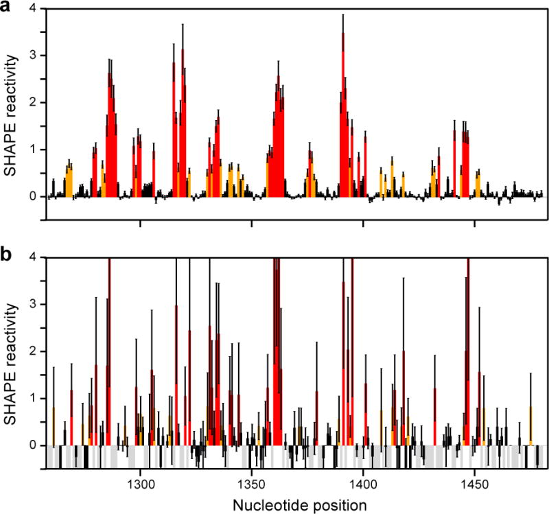
SHAPE-MaP reactivity profiles for the E. coli 16S rRNA. Reactivities below 0.4 are colored black, between 0.4 and 0.85 orange, and above 0.85 red. Gray bars indicate missing data points (corresponding to a background mutation rate above 5%, or read depth below 10). Error bars indicate standard errors. (a) High-quality reactivity profile. Shown is the final SHAPE reactivity profile for a portion of the 16S rRNA generated by comparing plus-reagent, minus-reagent, and denaturing control experimental samples with median read depths of 46,047, 36,704, and 22,531, respectively. (b) Poor-quality reactivity profile. The RNA is the same as that used to generate data shown in panel a but was sampled at median read depths of 647, 623, and 661 in the three experiments.

Images of the read depth versus nucleotide position for each RNA will be produced (Fig. 10). Histograms of mutation rates, read depths, SHAPE reactivities, and standard errors (useful for experiment troubleshooting) will be produced (Fig. 11B).

Figure 10.

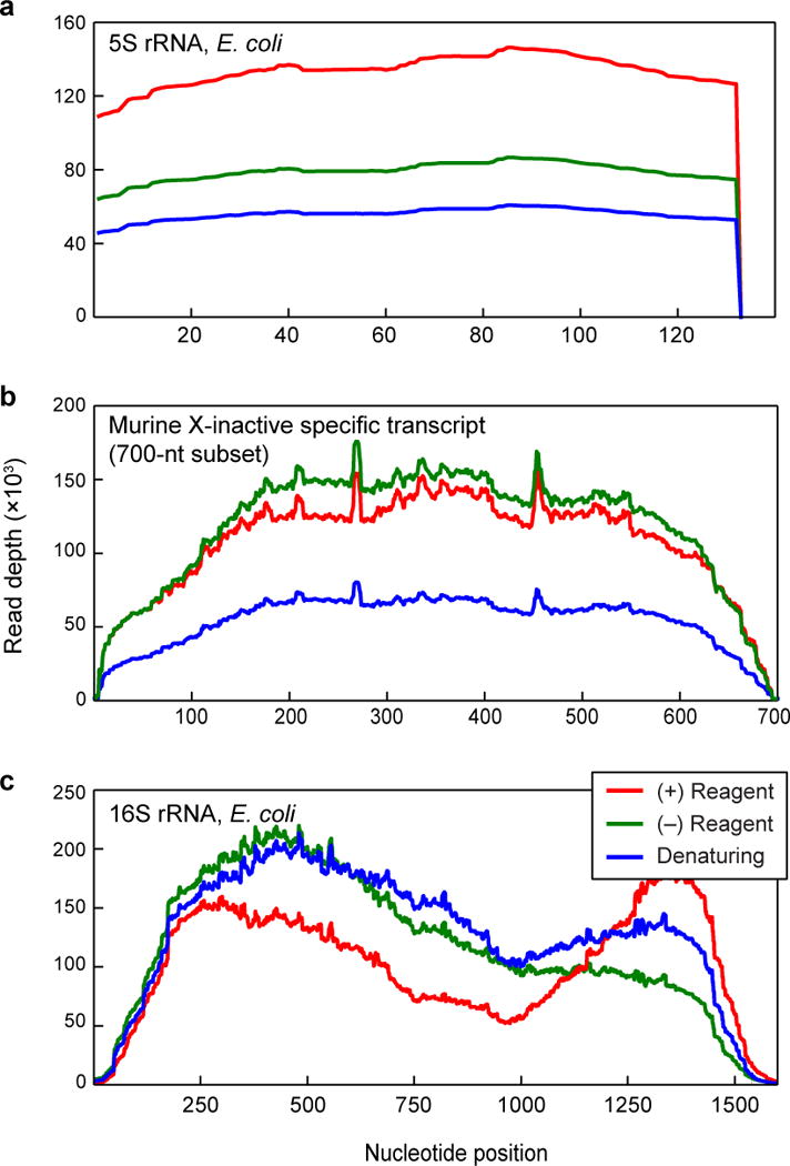
Read depth profiles. (a) Read depths obtained from an experiment using a single pair of directed primers (the Small RNA Workflow) against E. coli 5S rRNA, a short RNA. (b) Read depths obtained from an experiment targeting a specific region of a long noncoding RNA with the Amplicon Workflow. (c) Read depths obtained for the 16S rRNA from E. coli using the Randomer Workflow. Profiles for plus reagent (red), minus reagent (green), and denaturing control (blue) are shown for each workflow.

Figure 11.

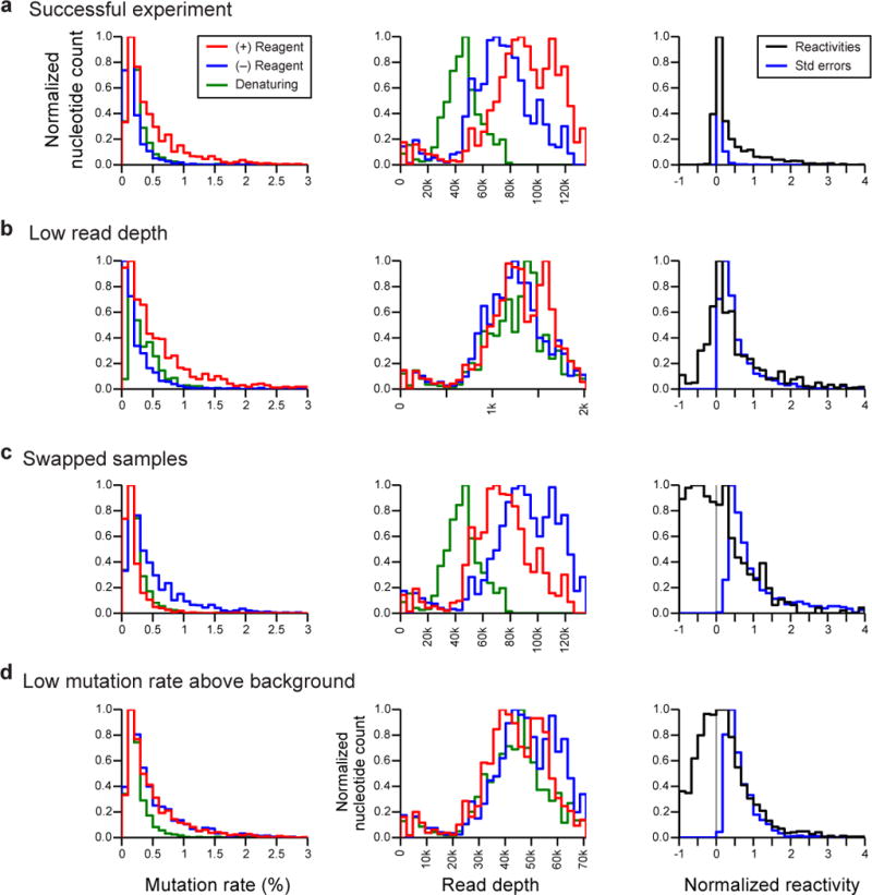
Troubleshooting, showing example data from the E. coli 16S rRNA. (a) Successful experiment. Failed experiments due to: (b) Low read depths. (c) Mislabeling of plus-reagent and minus-reagent samples. (d) Low levels of modification or mutation rates above background.

Intermediate files for each analysis stage will be written to disk (Table 3).

CRITICAL STEP: Analysis of the example ShapeMapper data requires 20 min on a 12-core, 2.93 GHz Dell C6100 server. This is a typical run-time for target RNAs less than 100,000 nucleotides and for the amount of data generated from a single MiSeq sequencing instrument run. Larger datasets or longer target sequences increase the run-time.

SuperFold analysis

• 39To model RNA structure, use the .map or .mapd file generated by ShapeMapper (see Box 3 for a description of file formats) in SuperFold by typing the command: SuperFold.py 16SrRNA.map

Box 3. SuperFold file formats.

Examples of file formats are included with the SuperFold executable. Descriptions of the formats are provided here.

Map file. A “.map” file is required to run SuperFold. This file is created automatically in the Results folder of ShapeMapper. The .map file is a tab-separated text file with four columns: Nucleotide number, SHAPE reactivity, Standard error, and Sequence. SHAPE reactivity and standard error values set to −999 are interpreted as no data.

MapD file. For three-reagent “differential” SHAPE folding, a “.mapd” file is required. In a differential experiment, the Python program differenceByWindowMap.py generates a differential SHAPE-MaP file (.mapd) from two .map files that report reactivities using the 1M6 and NMIA reagents. Use of the .mapd file in SuperFold results in incorporation of differential SHAPE reactivity into the SHAPE free energy term²¹. The .mapd file is a tab-separated text file with five columns: Nucleotide number, Differential SHAPE reactivity, Standard error, Sequence, and Z-factor. SHAPE reactivity and standard error values set to −999 are ignored.

SuperFold is typically run with default settings for folding window sizes.

Expected outcome

Three folders are created, called “fold_”, “partition_”, and “result_”, each underscore is followed by the name of the input .map file and a short signature created from a MD5 hash of the flags.

The parameters used to fold the RNA and the status of the run are written to the log file in the results directory.

Intermediate partition function calculations are written to the “partition” directory. These are useful for troubleshooting. If the run completes successfully, these can be deleted. Intermediate folds are written to the “fold” directory. These are also useful for troubleshooting. If the run completes successfully, these can be deleted.

Shannon entropy and SHAPE analyses, partition function arcs, and expanded regions are written to the results directory.

Text files reflecting Shannon entropy, partition function calculations, and minimum free energy structure (.ct format) are written to the results directory.

Secondary structure graphics and connectivity files for Shannon entropy/SHAPE regions are written to the regions subdirectory inside the results directory.

Timing

• RNA folding and modification

• Steps 1–12, 1 hour

• DNase treatment

• Steps 13–15, 1 hour

• MaP reverse transcription

• Steps 16–19, 4 hours (~1 hour hands-on time);

• Small RNA workflow

• Step 20A, 2 hours (~ 45 min hands on time);

• Amplicon workflow

• Steps 20B(i–v), 2 hours (~1 hour hands-on time); steps 20B(vi–xii), 2.5 hours (~1 hour hands-on time)

• Randomer workflow

• Steps 20C(i–iv), 3 hours (~30 min hands-on time); step 20C(v), 2.5 hours (~1 hour hands-on time)

• Quality control and sample dilution

• Steps 21–23, 2 hours (~1 hour hands-on time)

• Sequencing

• Step 24, 1–8 days depending on the sequencing platform.

• Run ShapeMapper

• Steps 25–38, 1 hour for example dataset (~15 minutes hands-on time)

• Run SuperFold

• Step 39, 1 hour or more depending on RNA size (~10 minutes hands-on time)

Troubleshooting

Troubleshooting tips for common SHAPE-MaP errors are outlined in Table 5.

Table 5.

SHAPE-MaP Troubleshooting

Step	Problem	Possible cause	Solution
20A(vii)	Low library yield	Size selection too stringent	Use a 1:1 or 1.2:1 ratio of beads to sample.
20C(iv)	Low dsDNA yield	Poor cDNA yield from reverse transcription	Use more RNA; do not exceed 5 μg.
			Increase the RT primer concentration by 10-fold. For the Randomer Workflow this will result in shorter sequencing libraries.
21	Low library yield	Failed Step 1 or Step 2 PCR	Optimize PCR conditions for each reaction individually before performing them in sequence.
			Some RNAs amplify better with a different ratio of cycles between Steps 1 and 2. Perform PCR using 20 cycles of Step 1 and 10 cycles of Step 2.
22	Extra peaks observed in Small RNA Workflow library	Non-specific primers	Redesign the [RNA-specific] and [RT primer] sequences of Step 1 primers with an online tool such as Primer-BLAST to avoid off-target binding. Test primers by performing Step 1 PCR for 25–30 cycles and verifying product on a gel or Bioanalyzer chip.
		Low Step 1 PCR input	Increase the number of Step 1 cycles to 20, reduce Step 2 PCR to 10 cycles.
		Incomplete conversion of Step 1 product to Step 2 product	Reduce the number of Step 1 cycles or carry less Step 1 product through to Step 2 PCR.
24	Few reads align to RNA of interest	Non-specific primers	Redesign PCR primers (Small RNA and Amplicon Workflows, see above); optimize RNA purification (Randomer Workflow).

Troubleshooting tips for common ShapeMapper errors are outlined in Table 6.

Table 6.

ShapeMapper Troubleshooting

Problem	Possible cause	Solution
No output files produced.	Missing pipeline binaries, file permissions not set correctly, missing files, incorrectly-formatted configuration file, or out of memory.	Ensure executable binary files trimPhred, parseAlignment, and countMutations are present in the ShapeMapper directory (see section on installing ShapeMapper). Check the log file (log.txt) in the run directory for details of the error. If running in a load sharing facility-enabled cluster computing environment, also check the output of the submitted job, which will display errors due to file permissions or memory issues that cannot be captured in the ShapeMapper log file.
Noisy reactivity profiles.	Incorrectly labeled samples, low read depths, poor signal above background (low RNA modification rate or cDNA mutation rate in SHAPE-modified sample), or DNA contamination.	Check mutation rate and depth histograms in RUN/output/reactivity_profiles to determine cause.
Missing samples.	Unbalanced sequencing library sample loading or failed PCR.	Quantify missing samples with a high-sensitivity assay and resequence. Redesign directed primers if necessary. Increase the amount of RNA in reverse transcription and increase the amount of first-strand cDNA in PCR.
Uneven read depth or regions of low depth.	RNA degradation, poor primer binding, or low RNA concentration.	Sequence using longer reads; use Nextera kits (if using the Illumina platform); use more RNA in reverse transcription; use a battery of paired PCR primers instead of random primers. For RNAs with regions of high AU-content, consider using the LNA+ random primers (Fig. 5).
No reactivity profiles produced, even though alignment files (./output/aligned_reads/*.sam) are present.	Sample name(s) in the “[profiles]” section of the configuration file do not exactly match the name(s) given in the FASTA reference sequence files (.fa).	Fix errors in the configuration file and rerun the generateReactivityProfiles stage.
Pipeline run incomplete, but no error message or unhelpful error message in the log file.	Out-of-memory error or other error that ShapeMapper does not currently identify.	Check the output from the ShapeMapper.py script itself, in addition to the log file (log.txt). Check the contents of the subfolders in the ./output/directory in order of module execution (Table 3). The first folder in which some or all of the expected output files are missing, blank, or empty indicates the stage that failed.

Troubleshooting tips for common SuperFold errors are outlined in Table 7.

Table 7.

SuperFold Troubleshooting

Problem	Possible cause	Possible solution
Error message: “Program X not found in the path”.	RNAstructure command-line tools not available to SuperFold.	Make RNAstructure accessible by adding it to the shell path.
Error message: “DATAPATH not set…”	RNAstructure DATAPATH is not set.	Use the export command to set the variable DATAPATH to the location of the RNAstructure data tables (see hardware setup).
Error message: “Unexpected character in…”.	Misformatted constraint file.	Check the input files for extra spaces or special characters.
Error message: “pK region file incorrectly…”.	Misformatted constraint file.	Check pseudoknot constraint file for formatting. See the example file.
No base pairs are found in the partition function.	Crash in the program partition gives empty output.	Set the –partitionWindowSize flag to 1200 and rerun SuperFold. Depending on the sequence, a large SHAPE penalty can cause partition to malfunction with large window sizes.

ANTICIPATED RESULTS

SHAPE-MaP allows measurement of RNA flexibility at single-nucleotide resolution for most nucleotides in an RNA. The experiment yields highly reproducible and quantitative information that enable accurate structure modeling and examination of RNA-ligand, RNA-RNA, and RNA-protein interactions. Successful completion of this experimental protocol yields deep sequencing libraries (Fig. 6) that are interpreted using automated post-sequencing processing using ShapeMapper to yield final SHAPE reactivities (Figs. 7 & 8). These SHAPE reactivities provide a starting point for modeling RNA secondary structure using SuperFold, which is optimized for long sequences (2000 nucleotides and much longer, but also works well for modeling shorter RNAs (Figs. 12 and 13). Distinct experimental workflows are optimized for probing small, low-abundance, or complex mixtures of RNA. Here we briefly present representative results obtained with two of the three workflows, the Small RNA and Randomer Workflows.

Figure 8.

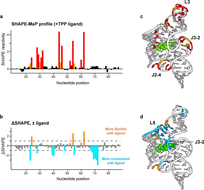
Nucleotide-resolution interrogation of RNA structure and ligand-induced conformational changes for the TPP riboswitch aptamer domain. (a) SHAPE profile produced using the Small RNA Workflow. (b) Difference SHAPE profile illustrating conformational changes induced in the TPP riboswitch upon ligand binding. (c) SHAPE-MaP reactivities superimposed on the structure⁵⁹ of the ligand-bound TPP riboswitch. Red, orange, and black correspond to high, moderate, and low reactivities, respectively, and correspond to reactivities shown in panel a. (d) Visualization of ligand-induced conformational changes on the TPP riboswitch structure. Reactivity changes (orange and blue) are the same as shown in panel b.

Figure 12.

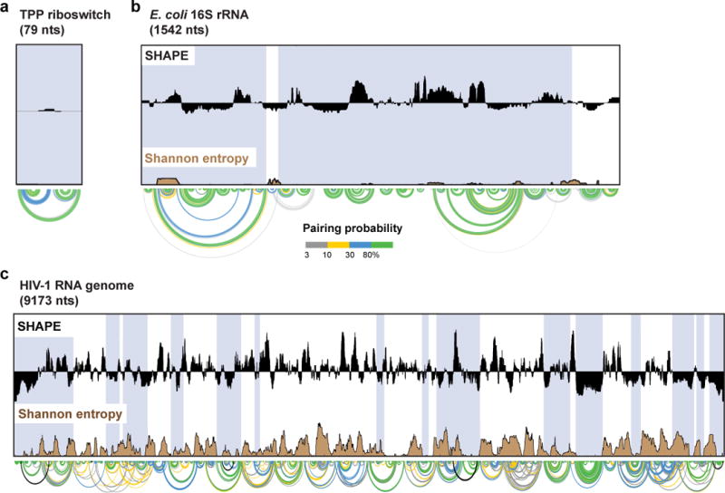
SuperFold analysis. Results from three RNAs: (a) TPP riboswitch, (b) E. coli 16S rRNA, and (c) HIV-1 RNA genome. SHAPE profiles are shown in black (as the median over a 51-nt window) relative to the global median; Shannon entropies are brown. Median SHAPE reactivities and Shannon entropies are shown on the same scale in all panels. Arcs illustrate base pairing probabilities with highly probable pairs emphasized in green. Manually added pseudoknots in the HIV-1 RNA are plotted as black arcs. Regions with both low SHAPE reactivity (corresponding to high levels of RNA structure) and low Shannon entropy (reflecting a well-determined structure) are emphasized with blue shading. Note that the TPP riboswitch and ribosomal RNAs are almost entirely comprised of low SHAPE/low entropy regions, whereas the HIV-1 RNA genome alternates between regions of well-determined structure and those without.

Figure 13.

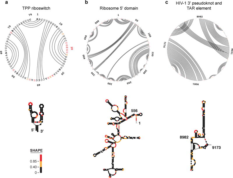
Secondary structure models for well-determined regions. (a) Predicted TPP riboswitch structure in its ligand-bound state. (b) 5′ domain of the E. coli 16S ribosomal RNA. (c) A well-determined structure within the HIV-1 RNA genome, containing a pseudoknot and the 3′ trans-activation response (TAR) element.

A SHAPE profile for the aptamer domain of the TPP riboswitch was readily obtained using the Small RNA Workflow. Using these data, secondary structure modeling for this riboswitch RNA improved from a base pair prediction accuracy of 73%, obtained using a nearest-neighbor thermodynamic algorithm alone, to 96%, using SHAPE-directed modeling²⁸. Observed reactivities correspond closely to those expected based on the local nucleotide flexibilities for the ligand-bound RNA (Fig. 8a,c). Reactive nucleotides fall in conformationally flexible single-stranded regions, especially the L3 loop and the J2-4 and J3-2 strands. Overall, relatively few nucleotides are reactive by SHAPE, consistent with the highly constrained conformation of this RNA. SHAPE-MaP also reveals fine differences corresponding to changes induced upon binding by the TPP ligand (Fig. 8b,d). Ligand interactions induce a large structural organization in the L5 loop and in the J3-2 elements in the ligand-binding pocket.

Large RNAs like the bacterial small and large ribosomal subunit RNAs (16S and 23S, respectively) are readily examined by applying the Randomer Workflow to total E. coli RNA (Fig. 9). Using random primers, both RNAs can be studied simultaneously with fully automated analysis involving approximately 3 days of hands-on experimental effort. The major post-processing requirement is that the per-nucleotide hit level be sufficiently high to permit full recovery of the underlying SHAPE data. In general, the hit level should be 5 or greater, corresponding to a read depth of 1–2,000²⁸.

Figure 9.

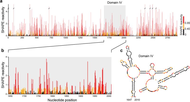
Representative SHAPE-MaP reactivity profile obtained using the Randomer Workflow. (a) SHAPE reactivities across the entire E. coli 23S rRNA obtained in a single experiment. (b) Expanded view of SHAPE reactivities for Domain IV of the 23S rRNA. (c) Accepted secondary structure of Domain IV colored by SHAPE reactivity. Reactive nucleotides (orange and red) occur predominantly in single-stranded regions.

The 23S rRNA subunit alone represents ~2,900 nucleotides of SHAPE reactivity information after computational data processing (Fig. 9a). Comparing the SHAPE reactivities for domain IV of the 23S rRNA with the accepted sequence covariation-derived structural model (Fig. 9b–c) shows good agreement. Regions involved in canonical base pairs have low SHAPE reactivity, indicating that they are structurally constrained. Conversely, single-stranded loop and bulge regions have high SHAPE reactivity, indicating structural flexibility. Because of the inherent scalability of the MaP approach, these data – spanning several thousand nucleotides – are as accurate at single-nucleotide resolution as are data from a short RNA, like the TPP riboswitch.

After the ShapeMapper analysis is complete, the rendered SHAPE reactivity profiles provide an clear view of the general success of an experiment (.pdf files in the “reactivity_profiles” folder). A successful experiment should have only a small number of negative gray bars (indicating no-data points), and small error bars (Fig. 7a).

The majority of SHAPE-MaP experiments are strikingly successful. The data obtained are reproducible, robust, correlate well with previous, well-validated approaches for SHAPE readout²⁸, enable consistent high-accuracy RNA structure modeling²¹ and recover detailed information about structural ensembles⁴⁸. In our laboratory, it is routine for full biological replicates, performed months apart by different individuals, to yield identical experimental results, within narrow error limits²⁸. However, when problems do occur, the SHAPE reactivity profiles, along with other ShapeMapper outputs, provide important clues for troubleshooting and identifying potential causes.

The most common cause of a failed SHAPE-MaP experiment is insufficient sequencing depth. SHAPE-MaP cDNA libraries sequenced to low depths do not produce high-confidence SHAPE reactivity profiles (as evidenced by large error bars, Fig. 7b) and, consequently, do not enable accurate structural modeling (see Figure 3 in the original SHAPE-MaP publication²⁸). We recommend sequencing to read depths above about 2,000 for each experimental condition to obtain high-confidence SHAPE reactivities and accurate structure models.

Read depths can be assessed directly by examining the profiles produced by ShapeMapper. For experiments using the Small RNA Workflow, a relatively flat depth profile is desirable and typically achieved (Fig. 10a). A depth profile with bumps or steps indicates possible off-target or non-specific primer binding. Enzymatic fragmentation and tagging (Nextera) results in lower read depth near the transcript ends due to the inability of the enzymes to cleave near the ends of a double-stranded DNA. In addition, read-depth profiles for libraries prepared in this way often exhibit a spikiness that likely results from sequence preferences during the fragmentation step. The Amplicon Workflow results in relatively flat profiles in the middle of a transcript (Fig. 10b), whereas the Randomer Workflow typically produce less even depth profiles (Fig. 10c) due to the differential efficiency of primer binding. Regions of low read depth, even if embedded in areas of high median read depth, do not produce reliable reactivity profiles by SHAPE or any other structure probing approach. Specially designed primers can improve or smooth the distribution of read depths for RNAs with AU-rich regions (Fig. 5)²⁸.

ShapeMapper produces multiple histograms useful for distinguishing successful from problematic experiments. For example, a successful experiment will show that the vast majority of nucleotides have read depths above 2000 (Fig. 11a, center panel); whereas an unsuccessful experiment (Fig. 11b, center panel) may have low overall sequencing depth. A successful SHAPE-MaP experiment also requires sufficient levels of SHAPE modification above background, efficient reverse transcription, and the absence of DNA contamination. In a successful experiment (Fig. 11a, right panel), reactivities are mostly positive, and the standard errors are smaller than most of the reactivities. Successful experiments are characterized by mutation rates in the no-reagent sample between 0 and 0.2%, a strong shift toward higher mutation rates in the plus-reagent sample, and a slight shift in the denaturing control sample (Fig. 11a, left panels). An example of low mutation above background, likely due to low levels of SHAPE modification, is illustrated in Fig. 11d, left panel. A noisy SHAPE reactivity profile (for example, Fig. 7b) is also indicative of a failed experiment.

The SuperFold analysis pipeline provides a solution to another challenge in analyzing large RNAs: automated visualization of secondary structures (Fig. 13). Two separate visualization approaches are implemented in SuperFold: (i) circle plots, which provide an impartial model-free view of secondary structure and enable rapid visualization of pseudoknots, and (ii) traditional secondary structure diagrams available through the Pseudoviewer⁵⁸ web service. Connectivity (.ct) and XRNA (http://rna.ucsc.edu/rnacenter/xrna/) files are provided that can be used as input to other structure visualization programs.

A melded Shannon entropy and SHAPE analysis (Fig. 12) is particularly useful for identifying regions of an RNA that have well-determined folds and for identifying parts of an RNA that merit detailed follow up analysis for function. Three different examples of expected output are shown: the E. coli thiamine pyrophosphate aptamer domain, the entire 16S rRNA, and the entire HIV-1 RNA genome (Fig. 12). Regions that contain both low Shannon entropy and low SHAPE reactivity appear to be highly likely to harbor functional elements^28,31. After expanding low Shannon entropy/SHAPE regions to include overlapping minimum free energy helices, almost the entirety of the TPP riboswitch and ribosomal RNAs are comprised of low Shannon entropy/low entropy regions (Fig. 12, purple shading), consistent with their known roles as RNAs whose function requires a specific well-defined fold. In contrast, the HIV-1 RNA genome has regions with low Shannon entropy and low SHAPE reactivity and also many regions that are predicted not to form well-defined structured states (Fig. 12c). Pairing probability arcs illustrate a relatively simple set of probable base pairs (derived from the partition function) for the TPP riboswitch and the 16S rRNA (Figs. 12a and 12b, see green arcs). In contrast, the HIV-1 RNA genome features both well-determined structural motifs and regions where the probability of formation of a single stable structure is low (Fig. 12c).

In sum, SHAPE-MaP and the ShapeMapper and SuperFold pipelines yield quantitative nucleotide-resolution RNA structural information, enable accurate secondary structure modeling, identify well-determined regions within large RNAs, facilitate discovery of novel functional RNA motifs, make possible deconvolution of sequence polymorphisms in a single experiment, detect diverse effects of ligand and protein binding, readily allow analysis of low-abundance RNAs, and scale gracefully from short RNAs to transcriptome-wide analyses, including in cells. We anticipate that SHAPE-MaP will contribute to deep understandings of the relationships between RNA structure and function.

References

- 1.Sharp PA. The centrality of RNA. Cell. 2009;136:577–580. doi: 10.1016/j.cell.2009.02.007. [DOI] [PubMed] [Google Scholar]
- 2.Dethoff EA, Chugh J, Mustoe AM, Al-Hashimi HM. Functional complexity and regulation through RNA dynamics. Nature. 2012;482:322–330. doi: 10.1038/nature10885. [DOI] [PMC free article] [PubMed] [Google Scholar]
- 3.Mauger DM, Siegfried NA, Weeks KM. The genetic code as expressed through relationships between mRNA structure and protein function. FEBS Lett. 2013;587:1180–1188. doi: 10.1016/j.febslet.2013.03.002. [DOI] [PMC free article] [PubMed] [Google Scholar]
- 4.Weeks KM. Advances in RNA structure analysis by chemical probing. Curr Opin Struct Biol. 2010;20:295–304. doi: 10.1016/j.sbi.2010.04.001. [DOI] [PMC free article] [PubMed] [Google Scholar]
- 5.Mortimer SA, Kidwell MA, Doudna JA. Insights into RNA structure and function from genome-wide studies. Nat Rev Genetics. 2014;15:469–479. doi: 10.1038/nrg3681. [DOI] [PubMed] [Google Scholar]
- 6.Kwok CK, Tang Y, Assmann SM, Bevilacqua PC. The RNA structurome: transcriptome-wide structure probing with next-generation sequencing. Trends Biochem Sci. 2015;40:221–232. doi: 10.1016/j.tibs.2015.02.005. [DOI] [PubMed] [Google Scholar]
- 7.Merino EJ, Wilkinson KA, Coughlan JL, Weeks KM. RNA structure analysis at single nucleotide resolution by selective 2′-hydroxyl acylation and primer extension (SHAPE) J Am Chem Soc. 2005;127:4223–4231. doi: 10.1021/ja043822v. [DOI] [PubMed] [Google Scholar]
- 8.Gherghe CM, Shajani Z, Wilkinson KA, Varani G, Weeks KM. Strong correlation between SHAPE chemistry and the generalized NMR order parameter (S2) in RNA. J Am Chem Soc. 2008;130:12244–12245. doi: 10.1021/ja804541s. [DOI] [PMC free article] [PubMed] [Google Scholar]
- 9.Wilkinson KA, et al. Influence of nucleotide identity on ribose 2′-hydroxyl reactivity in RNA. RNA. 2009;15:1314–1321. doi: 10.1261/rna.1536209. [DOI] [PMC free article] [PubMed] [Google Scholar]
- 10.McGinnis JL, Dunkle JA, Cate JHD, Weeks KM. The mechanisms of RNA SHAPE chemistry. J Am Chem Soc. 2012;134:6617–6624. doi: 10.1021/ja2104075. [DOI] [PMC free article] [PubMed] [Google Scholar]
- 11.Wilkinson KA, et al. High-throughput SHAPE analysis reveals structures in HIV-1 genomic RNA strongly conserved across distinct biological states. PLoS Biol. 2008;6:e96. doi: 10.1371/journal.pbio.0060096. [DOI] [PMC free article] [PubMed] [Google Scholar]
- 12.Gherghe C, et al. Definition of a high-affinity Gag recognition structure mediating packaging of a retroviral RNA genome. Proc Natl Acad Sci. 2010;107:19248–19253. doi: 10.1073/pnas.1006897107. [DOI] [PMC free article] [PubMed] [Google Scholar]
- 13.Archer EJ, et al. Long-range architecture in a viral RNA genome. Biochemistry. 2013;52:3182–3190. doi: 10.1021/bi4001535. [DOI] [PMC free article] [PubMed] [Google Scholar]
- 14.Spitale RC, et al. RNA SHAPE analysis in living cells. Nat Chem Biol. 2013;9:18–20. doi: 10.1038/nchembio.1131. [DOI] [PMC free article] [PubMed] [Google Scholar]
- 15.Tyrrell J, McGinnis JL, Weeks KM, Pielak GJ. The cellular environment stabilizes adenine riboswitch RNA structure. Biochemistry. 2013;52:8777–8785. doi: 10.1021/bi401207q. [DOI] [PMC free article] [PubMed] [Google Scholar]
- 16.McGinnis JL, Weeks KM. Ribosome RNA assembly intermediates visualized in living cells. Biochemistry. 2014;53:3237–3247. doi: 10.1021/bi500198b. [DOI] [PMC free article] [PubMed] [Google Scholar]
- 17.McGinnis JL, et al. In-cell SHAPE reveals that free 30S ribosome subunits are in the inactive state. Proc Natl Acad Sci. 2015;112:2425–2430. doi: 10.1073/pnas.1411514112. [DOI] [PMC free article] [PubMed] [Google Scholar]
- 18.Mortimer SA, Weeks KM. A fast-acting reagent for accurate analysis of RNA secondary and tertiary structure by SHAPE chemistry. J Am Chem Soc. 2007;129:4144–4145. doi: 10.1021/ja0704028. [DOI] [PubMed] [Google Scholar]
- 19.Deigan KE, Li TW, Mathews DH, Weeks KM. Accurate SHAPE-directed RNA structure determination. Proc Natl Acad Sci. 2009;106:97–102. doi: 10.1073/pnas.0806929106. [DOI] [PMC free article] [PubMed] [Google Scholar]
- 20.Hajdin CE, et al. Accurate SHAPE-directed RNA secondary structure modeling, including pseudoknots. Proc Natl Acad Sci. 2013;110:5498–5503. doi: 10.1073/pnas.1219988110. [DOI] [PMC free article] [PubMed] [Google Scholar]
- 21.Rice GM, Leonard CW, Weeks KM. RNA secondary structure modeling at consistent high accuracy using differential SHAPE. RNA. 2014;20:846–854. doi: 10.1261/rna.043323.113. [DOI] [PMC free article] [PubMed] [Google Scholar]
- 22.Underwood JG, et al. FragSeq: transcriptome-wide RNA structure probing using high-throughput sequencing. Nat Meth. 2010;7:995–1001. doi: 10.1038/nmeth.1529. [DOI] [PMC free article] [PubMed] [Google Scholar]
- 23.Kertesz M, et al. Genome-wide measurement of RNA secondary structure in yeast. Nature. 2010;467:103–107. doi: 10.1038/nature09322. [DOI] [PMC free article] [PubMed] [Google Scholar]
- 24.Lucks JB, et al. Multiplexed RNA structure characterization with selective 2′-hydroxyl acylation analyzed by primer extension sequencing (SHAPE-Seq) Proc Natl Acad Sci. 2011;108:11063–11068. doi: 10.1073/pnas.1106501108. [DOI] [PMC free article] [PubMed] [Google Scholar]
- 25.Incarnato D, Neri F, Anselmi F, Oliviero S. Genome-wide profiling of mouse RNA secondary structures reveals key features of the mammalian transcriptome. Genome Biol. 2014;15:491. doi: 10.1186/s13059-014-0491-2. [DOI] [PMC free article] [PubMed] [Google Scholar]
- 26.Rouskin S, Zubradt M, Washietl S, Kellis M, Weissman JS. Genome-wide probing of RNA structure reveals active unfolding of mRNA structures in vivo. Nature. 2014;505:701–705. doi: 10.1038/nature12894. [DOI] [PMC free article] [PubMed] [Google Scholar]
- 27.Ding Y, et al. In vivo genome-wide profiling of RNA secondary structure reveals novel regulatory features. Nature. 2014;505:696–700. doi: 10.1038/nature12756. [DOI] [PubMed] [Google Scholar]
- 28.Siegfried NA, Busan S, Rice GM, Nelson JAE, Weeks KM. RNA motif discovery by SHAPE and mutational profiling (SHAPE-MaP) Nat Meth. 2014;11:959–965. doi: 10.1038/nmeth.3029. [DOI] [PMC free article] [PubMed] [Google Scholar]
- 29.Vogel J, Hess WR, Börner T. Precise branch point mapping and quantification of splicing intermediates. Nucleic Acids Res. 1997;25:2030–2031. doi: 10.1093/nar/25.10.2030. [DOI] [PMC free article] [PubMed] [Google Scholar]
- 30.Ule J, Jensen K, Mele A, Darnell RB. CLIP: a method for identifying protein-RNA interaction sites in living cells. Methods. 2005;37:376–386. doi: 10.1016/j.ymeth.2005.07.018. [DOI] [PubMed] [Google Scholar]
- 31.Mauger DM, et al. Functionally conserved architecture of hepatitis C virus RNA genomes. Proc Natl Acad Sci. 2015;112:3692–3697. doi: 10.1073/pnas.1416266112. [DOI] [PMC free article] [PubMed] [Google Scholar]
- 32.Lavender CA, Gorelick RJ, Weeks KM. Structure-Based Alignment and Consensus Secondary Structures for Three HIV-Related RNA Genomes. PLoS Comput Biol. 2015;11:e1004230. doi: 10.1371/journal.pcbi.1004230. [DOI] [PMC free article] [PubMed] [Google Scholar]
- 33.Reuter JS, Mathews DH. RNAstructure: software for RNA secondary structure prediction and analysis. BMC Bioinf. 2010;11:129. doi: 10.1186/1471-2105-11-129. [DOI] [PMC free article] [PubMed] [Google Scholar]
- 34.McCaskill JS. The equilibrium partition function and base pair binding probabilities for RNA secondary structure. Biopolymers. 1990;29:1105–1119. doi: 10.1002/bip.360290621. [DOI] [PubMed] [Google Scholar]
- 35.Mathews DH. Using an RNA secondary structure partition function to determine confidence in base pairs predicted by free energy minimization. RNA. 2004;10:1178–1190. doi: 10.1261/rna.7650904. [DOI] [PMC free article] [PubMed] [Google Scholar]
- 36.Shannon E. A mathematical theory of communication. The Bell System Technical Journal. 1948;27:379–423. [Google Scholar]
- 37.Talkish J, May G, Lin Y, Woolford JL, McManus CJ. Mod-seq: high-throughput sequencing for chemical probing of RNA structure. RNA. 2014;20:713–720. doi: 10.1261/rna.042218.113. [DOI] [PMC free article] [PubMed] [Google Scholar]
- 38.Staple DW, et al. Fast gapped-read alignment with Bowtie 2. Nat Meth. 2012;9:357–359. doi: 10.1038/nmeth.1923. [DOI] [PMC free article] [PubMed] [Google Scholar]
- 39.Taylor AI, et al. Catalysts from synthetic genetic polymers. Nature. 2015;518:427–430. doi: 10.1038/nature13982. [DOI] [PMC free article] [PubMed] [Google Scholar]
- 40.Wang B, Wilkinson KA, Weeks KM. Complex ligand-induced conformational changes in tRNA(Asp) revealed by single-nucleotide resolution SHAPE chemistry. Biochemistry. 2008;47:3454–3461. doi: 10.1021/bi702372x. [DOI] [PubMed] [Google Scholar]
- 41.Warner KD, et al. Structural basis for activity of highly efficient RNA mimics of green fluorescent protein. Nat Struct Mol Biol. 2014;21:658–663. doi: 10.1038/nsmb.2865. [DOI] [PMC free article] [PubMed] [Google Scholar]
- 42.Mortimer SA, Weeks KM. C2′-endo nucleotides as molecular timers suggested by the folding of an RNA domain. Proc Natl Acad Sci. 2009;106:15622–15627. doi: 10.1073/pnas.0901319106. [DOI] [PMC free article] [PubMed] [Google Scholar]
- 43.Duncan CDS, Weeks KM. Nonhierarchical ribonucleoprotein assembly suggests a strain-propagation model for protein-facilitated RNA folding. Biochemistry. 2010;49:5418–5425. doi: 10.1021/bi100267g. [DOI] [PMC free article] [PubMed] [Google Scholar]
- 44.Grohman JK, et al. A guanosine-centric mechanism for RNA chaperone function. Science. 2013;340:190–195. doi: 10.1126/science.1230715. [DOI] [PMC free article] [PubMed] [Google Scholar]
- 45.Raabe CA, Tang TH, Brosius J, Rozhdestvensky TS. Biases in small RNA deep sequencing data. Nucleic Acids Res. 2014;42:1414–1426. doi: 10.1093/nar/gkt1021. [DOI] [PMC free article] [PubMed] [Google Scholar]
- 46.Weeks KM. Review toward all RNA structures, concisely. Biopolymers. 2015;103:438–448. doi: 10.1002/bip.22601. [DOI] [PMC free article] [PubMed] [Google Scholar]
- 47.Loughrey D, Watters KE, Settle AH, Lucks JB. SHAPE-Seq 2.0: systematic optimization and extension of high-throughput chemical probing of RNA secondary structure with next generation sequencing. Nucleic Acids Res. 2014;42 doi: 10.1093/nar/gku909. [DOI] [PMC free article] [PubMed] [Google Scholar]
- 48.Homan PJ, et al. Single-molecule correlated chemical probing of RNA. Proc Natl Acad Sci. 2014;111:13858–13863. doi: 10.1073/pnas.1407306111. [DOI] [PMC free article] [PubMed] [Google Scholar]
- 49.Nicholson BL, White KA. Functional long-range RNA-RNA interactions in positive-strand RNA viruses. Nat Rev Micro. 2014;12:493–504. doi: 10.1038/nrmicro3288. [DOI] [PMC free article] [PubMed] [Google Scholar]
- 50.Duncan CDS, Weeks KM. SHAPE Analysis of Long-Range Interactions Reveals Extensive and Thermodynamically Preferred Misfolding in a Fragile Group I Intron RNA. Biochemistry. 2008;47:8504–8513. doi: 10.1021/bi800207b. [DOI] [PMC free article] [PubMed] [Google Scholar]
- 51.McGinnis JL, Duncan CD, Weeks KM. High-throughput SHAPE and hydroxyl radical analysis of RNA structure and ribonucleoprotein assembly. Meth Enzymol. 2009;468:67–89. doi: 10.1016/S0076-6879(09)68004-6. [DOI] [PMC free article] [PubMed] [Google Scholar]
- 52.Watts JM, et al. Architecture and secondary structure of an entire HIV-1 RNA genome. Nature. 2009;460:711–716. doi: 10.1038/nature08237. [DOI] [PMC free article] [PubMed] [Google Scholar]
- 53.Steen KA, Rice GM, Weeks KM. Fingerprinting noncanonical and tertiary RNA structures by differential SHAPE reactivity. J Am Chem Soc. 2012;134:13160–13163. doi: 10.1021/ja304027m. [DOI] [PMC free article] [PubMed] [Google Scholar]
- 54.Mortimer SA, Weeks KM. Time-resolved RNA SHAPE chemistry. J Am Chem Soc. 2008;130:16178–16180. doi: 10.1021/ja8061216. [DOI] [PubMed] [Google Scholar]
- 55.Bai Y, Tambe A, Zhou K, Doudna JA. RNA-guided assembly of Rev-RRE nuclear export complexes. Elife. 2014;3:e03656. doi: 10.7554/eLife.03656. [DOI] [PMC free article] [PubMed] [Google Scholar]
- 56.Turner R, Shefer K, Ares M. Safer one-pot synthesis of the ‘SHAPE’ reagent 1-methyl-7-nitroisatoic anhydride (1m7) RNA. 2013;19:1857–1863. doi: 10.1261/rna.042374.113. [DOI] [PMC free article] [PubMed] [Google Scholar]
- 57.Ye J, et al. Primer-BLAST: a tool to design target-specific primers for polymerase chain reaction. BMC Bioinf. 2012;13:134. doi: 10.1186/1471-2105-13-134. [DOI] [PMC free article] [PubMed] [Google Scholar]
- 58.Byun Y, Han K. PseudoViewer: web application and web service for visualizing RNA pseudoknots and secondary structures. Nucleic Acids Res. 2006;34:W416–22. doi: 10.1093/nar/gkl210. [DOI] [PMC free article] [PubMed] [Google Scholar]
- 59.Serganov A, Polonskaia A, Phan AT, Breaker RR, Patel DJ. Structural basis for gene regulation by a thiamine pyrophosphate-sensing riboswitch. Nature. 2006;441:1167–1171. doi: 10.1038/nature04740. [DOI] [PMC free article] [PubMed] [Google Scholar]
Associated Data
This section collects any data citations, data availability statements, or supplementary materials included in this article.