

Abstract
Blood oxygenation level-dependent (BOLD) signal time courses in functional magnetic resonance imaging are estimated within the framework of general linear modeling by convolving an input function, that represents neural activity, with a canonical hemodynamic response function (HRF). Here we investigate the performance of different neural input functions and latency-optimized HRFs for modeling BOLD signals in response to vibrotactile somatosensory stimuli of variable durations (0.5, 1, 4, 7 s) in 14 young, healthy adults who were required to make button press responses at each stimulus cessation. Informed by electrophysiology and the behavioral task, three nested models with an increasing number of parameters were considered: a boxcar; boxcar and offset transient; and onset transient, boxcar and offset transient (TBT). The TBT model provided the best fit of the group-averaged BOLD time courses based on χ2 and F statistics. Only the TBT model was capable of fitting the bimodal shape of the BOLD response to the 7-s stimulus and the relative peak amplitudes for all stimulus lengths in key somatosensory and motor areas. This suggests that the TBT model provides a more comprehensive description of brain sensorimotor responses in this experiment than provided by the simple boxcar model. Work comparing the activation maps obtained with the TBT model with magnetoencephalography data is under way.
Keywords: General linear model, Transient response, Hemodynamic response function, Latency, Somatosensory system, Motor system
1. Introduction
The general linear model (GLM) is commonly used to describe the time course of the blood oxygenation level-dependent (BOLD) signal [1,2] in functional magnetic resonance imaging (fMRI). Within the GLM, an input function representing neural activity is convolved with a hemodynamic response function (HRF) [3], an impulse response function typically taken to be spatially invariant throughout the brain. Such modeling treats the BOLD response as the output of a linear time-invariant (LTI) system. A rectangular function, termed a boxcar, is often chosen as the input function with a width equal to the duration of the sensory stimulus or the behavioral task. The boxcar input function implies that the integrated BOLD signal increases linearly with the duration of the stimulus. This has been found for stimulus durations longer than approximately 3 s in the visual system [4–7] and may hold in the motor and auditory systems for even longer stimulus durations [5]. However, significant deviations from LTI properties have been reported for BOLD responses of the visual [5,6,8–16], motor [5,9,10,17], auditory [5,17,18] and somatosensory systems [19,20] for stimulus durations less than approximately 3 s. Moreover, such deviations have also been found for cognitive tasks [21]. Recognizing that the assumption of constant neural activity for a sustained stimulus is an oversimplification, a number of authors have suggested that neural transients or neural adaptation could explain, at least partially, such deviations from LTI properties [5,7,8,10,12,19–22]. These reports primarily focus on transient stimulus onset responses. Offset transients for sensory stimuli, however, have not been studied extensively with fMRI [12] despite the observation of sensory evoked offset responses in electroencephalography, e.g., in the auditory system [23], and event-related desynchronizations in magnetoencephalography (MEG) [24–26].
The objective of this study is to investigate how well the GLM can model the time courses of the BOLD signal specifically in the presence of both transient and sustained response components. Previously, Nangini et al. investigated the primary somatosensory responses to passively experienced vibrotactile stimulation with fMRI and MEG [19,20] and suggested to consider transient neural components. In these experiments, the fMRI signal showed substantial intersubject variability that was thought to occur at least partly due to fluctuations in attention. Because attention is known to modulate the BOLD response [27,28], we extended this work and developed an experiment to control for attention effects by instructing subjects to attend to the offset of the somatosensory stimulus and respond with a button press. We expected that, in such an experiment, transient onset and offset responses would encode the sensation of the environmental change, along with a sustained response associated with monitoring the sensation of the ongoing vibrotactile stimulus, and that these responses would be reflected in the fMRI signal. Accordingly, the fMRI time courses were fit using three nested models of the neural input: a boxcar (B), a boxcar and offset transient (BT), and a boxcar with onset and offset transients (TBT). We tested the hypothesis that the TBT model fits the observed BOLD time courses better than the B or BT models throughout the sensorimotor system. A boxcar with onset transient (TB) model was considered but initial investigations indicated that the offset transient was stronger than the onset transient. Therefore, the TB model was not investigated in detail.
In addition to refined modeling of the time courses of activation, the activation maps generated using the TBT model may provide a more comprehensive view of brain activity. The validity of the model can be further strengthened through correlation of transient and sustained components of the BOLD signal with corresponding electrophysiological measures of neural activity. For this purpose, MEG data have been recorded in the same participants with the same experimental paradigm. The comparison between the fMRI and MEG data will be presented elsewhere.
2. Materials and methods
2.1. Study design
Fifteen young adults (ages 20–38 years, eight female) participated in this study. The study was approved by the Research Ethics Board at Baycrest, and informed consent was obtained from each subject in written form. Four runs of fMRI time series data were collected in the presence of vibrotactile stimuli generated by a pneumatically driven membrane [29] vibrating at 22 Hz. In two runs, 45 trains of vibrotactile stimuli of 1-s, 4-s and 7-s duration were applied, with an interstimulus interval (ISI) of 10 s, to the palmar surface of the distal phalanx of the right index finger. In two additional runs, 20 stimuli with durations of 0.5 s and 1 s were presented, with 29.5- and 29-s ISI durations, respectively. The stimulus duration and ISI values were chosen to accommodate specific biophysical requirements for both fMRI and MEG data collections. It was assumed that, at a stimulus duration of 7 s, onset and offset transients of the BOLD response would be separated clearly based on initial simulations of BOLD response characteristics using a canonical HRF (see below). The shorter ISI was chosen to allow sufficient trials for robust signal averaging of the MEG data, whereas the longer ISI provided detailed sampling of the return of the BOLD response to baseline. Stimuli were presented in pseudorandom order for each run, and subjects were instructed to respond to the stimulus offset by pressing a button with their opposite (left) hand to maintain attention during each stimulus. Participants fixated their eyes on a white cross with a black background during the runs.
2.2. MR scanning
Scanning was performed on a 3-T MRI system (Trio; Siemens, Erlangen, Germany; VB15 software) using a 12-channel phased array head coil. A T1-weighted anatomical scan was acquired using the magnetization prepared 180° radiofrequency pulses and rapid gradient-echo [30] sequence with repetition time (TR)/echo time (TE)/flip/field of view (FOV)/matrix/bandwidth of 2 s/2.63 s/9°/25.6 cm/256×192/ 180 Hz/pixel in 6/8 partial Fourier mode. To improve the fitting performance of the GLM regression, temporal sampling of the BOLD time course was increased at the cost of a reduced FOV. A slab comprised of 16 contiguous, oblique coronal, 3-mm-thick slices was acquired using T2*-weighted echo planar imaging (EPI), with TR/TE/Flip/FOV/matrix/bandwidth parameter settings of 1 s/30 ms/50°/20 cm/ 64×64/2520 Hz/pixel. The slab location was chosen to cover major components of the central somatosensory and motor systems, including primary and secondary somatosensory cortices, primary motor areas and the thalamus. To aid in spatial registration of anatomical and fMRI data, a full brain oblique coronal EPI image with 33 6-mm-thick slices was also acquired, with TR/TE/Flip/FOV/matrix/bandwidth set to 2 s/30 ms/70°/20 cm/64×64/2520 Hz/pixel.
2.3. Data preprocessing
Prior to model fitting, the fMRI data were corrected for effects of heartbeat, respiration, slice timing and head motion using established preprocessing algorithms in analysis of functional neuroimages (AFNI) [31]. Each run was normalized to the mean pixel value over time and smoothed spatially using a Gaussian filter with 6 mm full width at half-maximum. The anatomical images were registered to the EPI images semiautomatically with a six-parameter rigid-body transformation. All runs for each participant with less than 1.5-mm translational motion, as determined by the AFNI volreg function, were further analyzed using MATLAB (Mathworks Inc., Natick, MA, USA). One participant with larger head movements had to be excluded from further analysis. In particular, fitting of the data to the GLM framework was achieved using the MATLAB function glmfit. To account for the effect of baseline signal modulation in the BOLD time courses, the trend in the time course of each run was eliminated by incorporating seven Lagrange polynomials, of orders 0 to 6, each spanning the duration of the run, in the GLM design matrix.
2.4. Data analysis
The observed time courses of the BOLD signal were fitted using the general linear model with three different neural input functions. The mathematical framework is summarized briefly below. A model indexed by l ∈{‘B’, ‘BT’, ‘TBT’} was fit for each participant p to the time course vector of the BOLD signal at brain voxel v as follows:
| (1) |
where is the design matrix containing the design function vectors for the given model and are the model parameters. The vector gives the error of the fit, which is assumed to arise from an independent, Gaussian random process.
The design matrix X(l) for an experimental run is given by the column-wise convolution:
| (2) |
where h is the chosen hemodynamic impulse response function (HRF) vector (independent of model, experimental design, participant and brain voxel). The set of matrices { :1≤k≤K} gives the model-dependent, stimulus-related idealized components describing successive trials in an experimental run, where K is the number of trials in a run. In particular, for the kth trial,
| (3) |
where Lk is the duration of the kth stimulus, ISI is the interstimulus interval and is a row-vector-valued model- and trial-dependent stimulus-related idealized function (SRIF) representing the neural input:
| (4) |
For this study, three models were considered. For the first model (l=‘B’), a single boxcar function was used:
| (5) |
where u(n) is the unit step function. The second model (l=‘BT’) consisted of a boxcar function coupled with a Kronecker delta function δ(n) at the offset of the stimulus:
| (6) |
The third model (l=‘TBT’) consisted of a boxcar function and two delta functions, one at the stimulus onset and the other at the stimulus offset:
| (7) |
The fact that the B and BT functions are subsets of the TBT functions (i.e., the models are “nested”) facilitates the use of certain statistical tests described below. The offset transient was added first because initial pilot data indicated that offset transients were stronger than onset transients for the fMRI experiment under study. Before fitting, all runs of the same participant were concatenated in time.
During initial investigation, it became apparent that a single HRF h with constant latency (defined as the time required for the HRF to achieve its maximum value) was unable to model the variable location of sharp transient peaks in the BOLD time courses accurately. Therefore, we optimized the latency for each participant p and voxel v. The shape of h was defined by the “Cox special function” hCox[n] (as implemented in AFNI) with the following parameter settings: a peak amplitude of one, a rise time rt=3.5 s, a fall time ft=5 s, an undershoot us=0.2 and a restore time ret=15 s:
| (8) |
where z(x) = 0.50212657·(tanh(tan(0.5π·(1.6x−0.8))) + 0.99576486).
Latencies of the HRF peak in the range from 3.5 s to 8.5 s in 0.25-s steps were implemented by time-shifting the above function by a delay S (i.e., hS [n]=hCox [n−S]), resulting in 21 design matrices with different latencies. In this process, the SRIF and HRF were up-sampled by a factor of 4, yielding functions sampled at an effective interval of 0.25 s. Delta functions in the SRIFs were replaced by impulses 0.25 s wide and four times the height (to preserve their area). After executing the convolution, the resulting design matrices were down-sampled to the original TR value of 1 s. The optimal delay was determined for each voxel in each participant using the TBT model and a gradient search procedure starting at an HRF latency of 6.0 s minimizing the mean square error between the estimated time course of the fitted model and the BOLD time course. The optimal latencies found with the TBT model were included when fitting the other two models to prevent physiologically unreasonable latency values from improving the fit of the other two models. Without this procedure, for example, unreasonably long latencies were observed for the B model as it attempted to compensate for the offset transient.
To visualize and compute statistics comparing observed BOLD time courses and time courses estimated by the fitted models, measured and estimated time courses were averaged over both participants and trials for each stimulus duration d∈{1,4,7,0.5 (runs 3 and 4),1 (runs 3 and 4)}, yielding the grand average time courses:
| (9) |
where and are the BOLD signal response and the estimated time course of the kth stimulus at voxel v, Dk gives the temporal onset of the kth stimulus and P is the total number of participants. was extracted from , where are the estimated model parameters. The FShiftS{·} operator was employed to temporally align time courses of participants with differing latencies to an effective hemodynamic latency of 6.0 s via linear interpolation. Standard errors of the average time courses were also computed.
Averaging across participants was preceded by transforming T1 images and functional data to Talairach coordinates using the AFNI @auto_tlrc function with the TT_avg152T1 template. Finally, prior to computation of statistics, grand averages for each stimulus duration were concatenated, yielding and .
To quantify the goodness of fit of model estimates to grand average observed data, reduced χ2 values were calculated for each model l and voxel v:
| (10) |
where is the degrees of freedom associated with fitting model l obtained by subtracting the number of model parameters from the number of samples in the observed grand average time course. This number is dependent on voxel v because only samples where all subjects could contribute to the statistic without extrapolation of the latency corrected individual time courses were included. In addition, a set of extra sum-of-squares (ESS) F tests [32] for nested models was computed to find statistically significant improvements of models BT versus T, TBT versus BT, and TBT versus B:
| (11) |
| (12) |
| (13) |
where is the sum-of-squares of the residual of the grand average observed time course ỹv with respect to the grand average estimated time course . Histogram distributions of and (Fl,l′)v were computed for voxels considered active in any of the three components of the TBT model (see below).
To visualize the location of statistically significant coefficients obtained from model fitting, statistical parametric maps (SPMs) for the group of participants were computed. For each voxel and stimulus-related parameter from each model, the significance of the average estimated model parameter over all participants (n=14) was tested (against the null hypothesis of zero) using a t test with 13 degrees of freedom. To account for the varying number of stimulus-related parameters in each model, different significance thresholds were chosen according to Bonferroni correction: α=0.0133 for the TBT model, α=0.025 for the BT model and α=0.05 for the B model. In addition, only clusters of 50 voxels or more were retained to correct for multiple comparisons due to the number of voxels analyzed. SPMs were combined for visualization into a single color-coded map indicating the parameters of each of the three models that were found to be significantly active. This approach focused intentionally on the statistical significance of the estimated model parameter values, rather than their magnitude or sign.
A group analysis of this data is limited in terms of the precise local origin of signals. Therefore, a region-of-interest (ROI) analysis was also performed to study the origin of the TBT model components in individual subjects. The S1 and M1 areas contralateral to the stimuli were manually defined by painting the post- and precentral gyri, respectively, in axial slices from superior Talairach coordinates 45 mm to 65 mm in each subject. A false discovery rate of 0.05 was used to determine significant activation within S1 and M1, which was then analyzed based on histograms of component coefficients for both regions. For each brain region and for each subject, a particular GLM component was classified as positive (negative) if the directionality of the effect was observed in more than 90% of activating voxels.
3. Results
Figs. 1 and 2 show examples of fitted curves overlaid on group- and trial-averaged fMRI time courses from selected voxels in brain regions of interest: primary and secondary somatosensory cortices (S1 and S2, respectively), primary motor cortices (M1), supplementary motor areas (SMA) and the thalamus (Thal). Fig. 1 displays the fitted curves and experimental data for each stimulus length and trial type, whereas Fig. 2 provides an enlargement for the longest stimulus duration (7 s) only. For this stimulus length exceeding the width of the HRF, the experimental data show bimodal BOLD responses for many of the brain regions of interest, suggesting that the underlying neural activity indeed contains transient components. These two figures illustrate visually that only the TBT model is able to match both the amplitudes at different stimulus lengths (Fig. 1) as well as the bimodal nature of the 7-s stimulus (Fig. 2). The values, Talairach coordinates and group-averaged HRF latencies for these voxels are given in Table 1. The values for the TBT model are close to 1 or an ideal distribution. Except for contralateral primary motor cortex (M1c), values for the TBT model indicate better fitting of the data than what was obtained using the other two models.
Fig. 1.

Group-averaged time courses of the BOLD response in eight example voxels from different regions of the somatosensory–motor system: primary somatosensory cortex (S1), secondary somatosensory cortex (S2), primary motor cortex (M1) contralateral(c) or ipsilateral (i) to the stimulus, supplementary motor area (SMA) and thalamus (Thal). For each voxel, all five responses to the 1-s, 4-s and 7-s stimuli with 10-s ISI and 0.5-s and 1-s stimuli with 30-s ISI are shown (stimulus lengths are marked above the time axis as thick black lines). Fitted curves are also shown in each case for the boxcar (B), boxcar–offset transient (BT) and onset transient–boxcar–offset transient (TBT) models.
Fig. 2.

Group-averaged time courses of the BOLD response and associated fitted curves for the B, BT and TBT models for the same voxels and representation format as given in Fig. 1. Only the experimental data and fitted curves for the 7-s stimulus duration are shown here, allowing the bimodal response to be observed clearly.
Table 1.
Talairach locations, values and latencies for eight voxels in selected brain regions
| Anatomical area | LPI Talairach coordinates/mm |
|
HRF latency/s | |||
|---|---|---|---|---|---|---|
| B model | BT model | TBT model | ||||
| S1c | (−50, −32, −52) | 4.3 | 2 | 0.6±0.1 | 5.1±0.3 | |
| S1i | (54, −32, 52) | 4.5 | 2.1 | 0.9±0.1 | 5.4±0.4 | |
| S2c | (−58, −24, 16) | 9.5 | 3.6 | 1.2±0.1 | 4.3±0.2 | |
| S2i | (62, −24, 18) | 7.7 | 2.5 | 1.0±0.1 | 4.6±0.3 | |
| M1c | (−32, −28, 54) | 2.2 | 2.1 | 1.8±0.2 | 5.5±0.5 | |
| M1i | (50, −28, 54) | 4.8 | 2 | 1.0±0.2 | 5.4±0.4 | |
| SMA | (2, −2, 50) | 8.1 | 1.4 | 0.8±0.1 | 4.3±0.2 | |
| Thal | (8, −8, 6) | 9.8 | 2.6 | 1.2±0.1 | 4.9±0.2 | |
The error of the values is estimated as the standard deviation of the theoretical distribution with the given mean. The standard error of the mean is given for the latencies.
Fig. 3 shows the distributions of the computed values for each model for all voxels within the significantly activated areas identified by the TBT model (10 482 voxels, see below). The mean, median and standard deviation of these distributions are 4.05, 3.62 and 1.85 for the B model; 1.71, 1.62 and 0.56 for the BT model; and 1.12, 1.07 and 0.31 for the TBT model, respectively. The theoretical distribution for 90 degrees of freedom is also shown for comparison. The TBT model is closest to the theoretical distribution and outperforms the BT and B models.
Fig. 3.
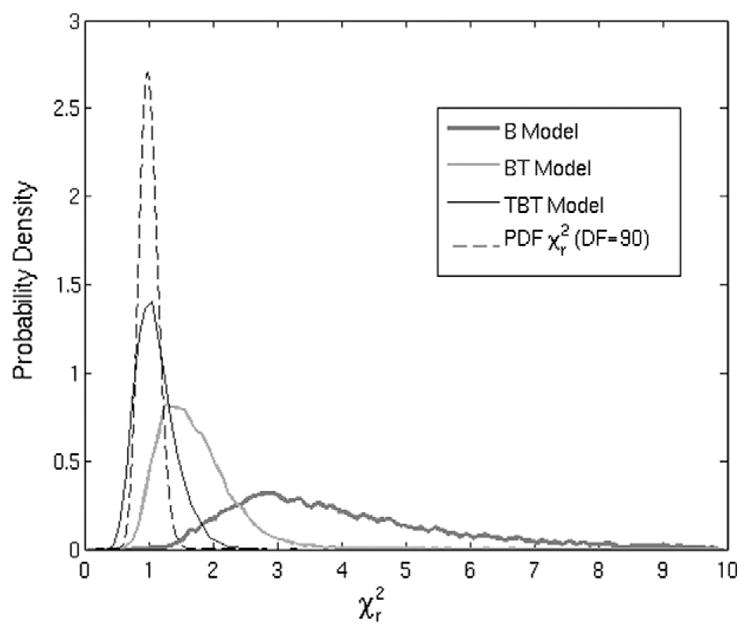
Distributions of the values for all voxels active in the TBT model for each model in comparison to an ideal distribution with 90 degrees of freedom.
The improved fitting provided by the TBT model was also analyzed based on ESS F tests. Fig. 4 illustrates the cumulative distributions of F values for comparing model TBT versus BT, TBT versus B, and BT versus B. These F distributions are based on the same data as the distributions. Because each curve rises steeply as a function of F value, a logarithmic scale is provided for the horizontal axis. In addition, two vertical lines indicate the range of F that correspond to α=0.05: F(0.95, 1, 84) represents the lower bound for a statistically significant reduction in residual variance for models that differ in one estimation parameter (e.g., BT vs. B) with 84 degrees of freedom, and F(0.95, 2, 104) is the analogous parameter considering models that differ by two experimental parameters (TBT vs. B) with 104 degrees of freedom. The values of 84 and 104 are the minimum and maximum number of degrees of freedom occurring among the analyzed voxels. F distributions shifted more to the right on this plot indicate greater statistical significance. The positions of the curves with respect to the thresholds indicate a highly significant reduction in residual variance obtained for the majority of voxels by moving from the standard B model to models containing additional transient components. Moving from the B to the TBT model or from the B to the BT model provides similarly large variance reductions, with the former providing slightly more benefit. The improvements for the TBT over the BT model were noticeable, however less pronounced. Specifically, less than 7% of voxels exhibit a reduction in variance that is not statistically significant at a level of P=.05. Fig. 4 also indicates that even if there was some uncertainty about the precise location of the statistical thresholds (e.g., due to potential noise correlations in the data that could perturb the estimated degrees of freedom), significant fit improvements by including transient components would likely still be observed in the majority of active voxels.
Fig. 4.
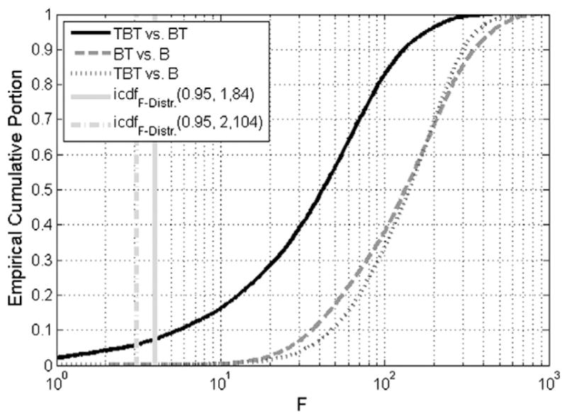
Empirical cumulative distributions of F values for all voxels active in the TBT model for model comparisons TBT vs. BT, TBT vs. B, and BT vs. B. As a marker of significance, the F values of the inverse cumulative distribution function (icdf) for 0.95 are given for the range of degrees of freedom within these voxels, which correspond to a P value of .05.
In Fig. 5A, the locations of the selected voxels of Figs. 1–2 are shown as 3×3×3 voxel neighborhoods projected onto representative axial, sagittal and coronal sections in Talairach space. Fig. 5B contains the spatial activation pattern for each model in each row for the same sections. The activation patterns for the BT and TBT model have been compressed into single maps by color-coding as described in the Methods section. The activated area was smaller for the B model than for the BT and TBT models despite conservative multiple comparison correction. The numbers of activated voxels were 7737, 11 921 and 10 482 for B, BT and TBT, respectively. The number of activated voxels was higher for the BT model than for the TBT model, which is not surprising given that many voxels are not significantly activated in the onset T component and the conservative multiple comparison correction. It is also evident that the interpretation of the nature of the activation changes depends on which model is being considered. For example, most voxels that are active in the B model are found to be active only in the transient components of the BT and TBT models. Very few areas, for example, a small cluster in the M1/S1 area contralateral to the stimulus, contained significant boxcar activation without significant transient components as assessed by the TBT model. This was the only region that was negatively activated during stimulation (i.e., reduced BOLD response during stimulation relative to baseline). All other regions activated positively with respect to baseline within the TBT model (Fig. 2). The TBT model showed that these other regions were activated either by the offset transient or, in areas such as bilateral S2 and thalamus, by both onset and offset transients.
Fig. 5.

(A) Projection of the locations of the example voxels (3×3×3 neighborhood) onto axial, sagittal and coronal slices intersecting at [−44, −34, 56] in LPI Talairach space (cross bars center). (B) Maps of significantly activated voxels for the three models with particular combinations of activation color coded (B, boxcar only; offT, offset transient only; BT, boxcar and offset transient only; onT, onset transient only; TB, onset transient and boxcar only; TT, onset and offset transient only). (C) HRF latency map for all voxels active in the TBT model. In (B) and (C), the activation maps are shown at a significance level of P<.05, including corrections for multiple comparisons.
Allowing the latency of the HRF maximum to shift was an important requirement for capturing the transient activation peaks accurately. Fig. 5C maps HRF latency values indicating that primary somatosensory and motor areas have an intermediate latency of approximately 5.5 s, whereas S2, SMA and brain stem regions have a shorter latency of 4–4.5 s. Long latencies (6–7 s) were observed in particular in the posterior cingulate region.
The results of the ROI analysis are summarized in Fig. 6. Histograms of statistically significant TBT model component coefficients are displayed for the group data (using the union of all individual subject masks for S1 and M1) in the top row; the middle and bottom rows contain similar histograms specific for the S1 and M1 regions using the pooled data (counts of significant voxels from each subject). The top row is consistent with the activation map in Fig. 5 and with the mean (or the asymmetry) in the individual subjects. As could be expected, the distributions of the individual subject data are much wider. They are not restricted to just positive or just negative values and become bimodal because coefficients of smaller magnitude are less likely to reach significance. Furthermore, the width of these distributions is largely due to intersubject variability. Intrasubject variability is much less as indicated by the fact that GLM components could be classified as positive (negative) in 4 (2), 1 (7) and 5 (2) subjects in S1 regarding the onset, boxcar and offset components, respectively. In M1, the respective numbers were 2 (3), 1 (8) and 6 (4). The classification of components from the same subject was highly consistent between S1 and M1. By category, 2 (2), 1 (7) and 4 (2) subjects classified in M1 could be classified in the same category in S1.
Fig. 6.

Histograms of TBT model coefficients for significantly activated voxels (see Methods section) in the group (top row) and for individual subjects (data pooled) in S1 and M1 contralateral to the stimulus. S1 and M1 were manually segmented for each subject.
4. Discussion
The results of this study suggest that the GLM framework incorporating the TBT model accounts well for the observed group-averaged BOLD fMRI time courses for varying somatosensory stimulus durations in this experiment. Overall, compared to the results obtained with the B and BT models, the histogram of TBT model was closest to theoretical expectations for a good model, confirming the hypothesis put forth in the Introduction. The F test results of Fig. 4 provide secondary support for this assertion.
Figs. 1–5 are also consistent with the notion, previously stated by others [5,8,10,12,19,20,22], that nonlinearity in BOLD fMRI studies associated with short sensory stimulus durations can be accounted for by a superposition of linear processes represented here by the transient and sustained components of the neural input function. It is possible that a nonlinear model, potentially including a nonlinear hemodynamic response, for example, would also be able to explain the data. Our analysis indicates merely that this may not be necessary in the large volume of brain with values close to 1 in the TBT model. Different effects could be important in other brain regions or for individual participant data, which are currently being investigated.
Extending the GLM approach, we utilized the HRF latency as an additional parameter for each volume element. The spatial variability and participant dependence of the HRF latency are important issues for functional brain imaging and remain to be explored extensively. Our latency maps in Fig. 5C are in basic agreement with the literature [33–35]. Our experience from the present work is that both the appropriate model of neural activity and the appropriate spatial variations in HRF latency are required for optimal fitting of fMRI data. However, as indicated by others [33], the regional variations in HRF latency arising from associated variations in brain vasculature should be considered as a confound for applications of mental chronometry [36,37], in which the time intervals between BOLD responses from different brain regions are thought to reflect mental processing. Absolute latencies as presented in Fig. 5C are more consistent with regional vascular differences than with a chronometric picture of task-related neural activity given that, for example, in this study, S2 has a shorter latency than S1 and that the time scales of the latency variations are far longer than for common neuronal processing.
The spatial patterns of transient and sustained components determined through the use of the TBT model are consistent with other functional neuroimaging literature. Of particular interest is S1c, the primary cortical area responding to a contralateral somatosensory stimulus [19,20,29], which has been shown to behave similarly to other primary sensory areas with respect to the linearity of the BOLD response as a function of stimulus duration [5]. In the context of our models, the boxcar component is the conventional function used in GLM analysis of fMRI data and for assessments of linear time invariance. For our data, the TBT model did not find a significant B component for almost all of the studied brain including the chosen S1c voxel. This is in agreement with the findings of Nangini et al. [20] that the fMRI response to 0.2-s, 0.5-s and 1-s stimuli is dominated by transient responses. An earlier study by Nangini et al. [19] investigated stimuli up to 20 s in duration and found that a model with an onset transient and a boxcar component fit the observed BOLD responses better than a pure boxcar model. While a pure transient model was not investigated in this prior study, the sustained, boxcar component was easily visible at such a long stimulus duration. Because the longest stimulus duration in the present study was 7 s, there may not have been adequate sensitivity to observe this boxcar component. Another possibility is that the button press task, which focused attention on the onset and offset of the stimulus, reduced the boxcar component to insignificant levels through top-down executive processing. In addition, the task adopted in the present work involved a button press response with the hand that was not stimulated, whereas no task or attention was required in Nangini et al. [19,20]. This task could have caused suppression of the sustained B component contralateral to the stimulus (see below). These differences in task may explain why Figs. 1, 2 and 5 highlight predominantly the transients, whereas Nangini et al. [19,20] observed both an onset transient and a more substantial sustained component.
Fig. 5B illustrates that offset transient (T) activations within the TBT model capture important areas of the motor network such as SMA and premotor areas that do not show onset T activation. This was expected given that the offset T also reflects the button press. Comparing our results to studies that do not include motor responses would certainly be of interest. Matching the attention conditions between experiments, however, would be a major challenge.
Interestingly, although the analysis indicates significant improvements in many contralateral S1 voxels for the TBT model over the BT model, the group t test does not show significant onset T activation in these voxels but only offset T activation (Fig. 5B). This indicates that the group t test approach to determine activation is not as sensitive to detect activations as an analysis of the group-averaged time courses would be. In the hemisphere contralateral to the button press (S1i), both onset and offset T activations were found to be significant. This was an unexpected finding given that the main activation for the stimulus onset was expected in the hemisphere contralateral to the stimulus and may be a consequence of the attention demanding task. In MEG with an equivalent experimental condition, we recently found ipsilateral activation under attention but not in an ignore control condition [26]. In addition, interparticipant variability was less on the ipsilateral side (S1i) as compared to the contralateral side (S1c in Fig. 2). In the S2 regions, onset and offset T responses were observed bilaterally (Figs. 2 and 5B) in agreement with previous studies [27] and the fact that each S1 area has efferents connecting to the S2 areas on both sides of the brain [38].
An interesting finding is the cluster of negative BOLD activation in the neighborhood of the M1 area contralateral to the stimulus and ipsilateral to the motor response. The investigation of the individual subject data [39] revealed that the effect is not limited to M1 but is also prevalent in S1. The group histogram showed no activation for the onset transient, negative activation for the boxcar component and positive activation for the offset transient. These results reflect the approximate mean values of the individual subject histograms. The individual subject data additionally showed that both positive and negative activations occurred for each component in individual subjects. However, within single subjects, a tendency could be observed to activate predominantly negatively or positively with the same directionality in both S1 and M1. This tendency was particularly pronounced for the negative boxcar component. A negative BOLD response is well known in M1 for ipsilateral motor activity [28,40] or in ipsilateral S1 and bilateral M1 for unilateral somatosensory stimulation [41]. However, it has not previously been reported that this negative response is predominantly linear with respect to stimulus length. This finding supports the notion that the ipsilateral M1/S1 negativity for motor tasks is potentially not driven by the motor activity itself, but rather by processes such as stimulus monitoring or motor preparation.
Among the eight example voxels shown in Figs. 1–2, the gain of the TBT model over the BT model is the lowest for the SMA. This is consistent with the notion that the SMA is particularly important for motor preparation for the button response and less so for the perception of simple somatosensory stimulation. In the thalamus, a large area of onset and offset activation is found, which reflects the involvement of the thalamus in both somatosensory and motor activity. However, even the TBT model could not separate motor and sensory pathways within the thalamus. One possibility to provide a general increase in spatial resolution would be to conduct subsequent studies at ultra-high magnetic field (e.g., 7 T or greater).
Despite these discussions, it still remains to be shown definitively that the input function components within the TBT model are indeed of neural origin. A recent conference presentation [42] has shown, for example, that transients found with gradient-echo BOLD did not occur with spin echo for a 30-s motor task at 3 T. This indicates that at least part of the transient signal could be due to a vascular effect, given that the spin-echo technique is less sensitive than the gradient-echo technique to BOLD signal effects in draining venules and veins. To provide further evidence that the components of the neural input functions do indeed reflect neural activity, additional work is required to study fMRI results in relation to other noninvasive measurements of brain activity in humans that do not rely on the neurovascular coupling mechanism, e.g., electroencephalography [4] or MEG. For this purpose, MEG data have been acquired for these specific participants under the same experimental conditions described in this study. Correlations between the MEG data and the components of the TBT model will be reported in a future publication.
In summary, this work shows that interesting new insights into the functioning of the brain can be gained from latency optimized models that include transient in addition to boxcar activations. While the importance of transient responses in BOLD fMRI has been recognized primarily for the visual system, little work has been done to investigate their nature and importance in the somatosensory system. While ignoring transients will potentially produce misleading results when interpreting maps of brain activity, no additional features such as nonlinear hemodynamics may be needed to characterize BOLD fMRI response characteristics with varying stimulus duration completely within the linear time-invariant framework. Further studies into the nature of transient fMRI responses are in progress.
Acknowledgments
The authors would like to acknowledge funding from the Canadian Institutes of Health Research (Grant MOP84447). We also thank the Heart and Stroke Foundation Centre for Stroke Recovery for general support, the donors of the Edward Christie Stevens Fellowship for supporting Michael Marxen and the Natural Sciences and Engineering Research Council (NSERC) of Canada for supporting Ryan Cassidy.
References
- 1.Kwong KK, Belliveau JW, Chesler DA, Goldberg IE, Weisskoff RM, Poncelet BP, et al. Dynamic magnetic resonance imaging of human brain activity during primary sensory stimulation. Proc Natl Acad Sci USA. 1992;89(12):5675–9. doi: 10.1073/pnas.89.12.5675. [DOI] [PMC free article] [PubMed] [Google Scholar]
- 2.Ogawa S, Lee TM, Kay AR, Tank DW. Brain magnetic resonance imaging with contrast dependent on blood oxygenation. Proc Natl Acad Sci USA. 1990;87(24):9868–72. doi: 10.1073/pnas.87.24.9868. [DOI] [PMC free article] [PubMed] [Google Scholar]
- 3.Friston KJ, Holmes AP, Poline JB, Grasby PJ, Williams SC, Frackowiak RS, et al. Analysis of fMRI time-series revisited [see comment] Neuroimage. 1995;2(1):45–53. doi: 10.1006/nimg.1995.1007. [DOI] [PubMed] [Google Scholar]
- 4.Boynton GM, Engel SA, Glover GH, Heeger DJ. Linear systems analysis of functional magnetic resonance imaging in human V1. J Neurosci. 1996;16(13):4207–21. doi: 10.1523/JNEUROSCI.16-13-04207.1996. [DOI] [PMC free article] [PubMed] [Google Scholar]
- 5.Soltysik DA, Peck KK, White KD, Crosson B, Briggs RW. Comparison of hemodynamic response nonlinearity across primary cortical areas. Neuroimage. 2004;22(3):1117–27. doi: 10.1016/j.neuroimage.2004.03.024. [DOI] [PubMed] [Google Scholar]
- 6.Vazquez AL, Noll DC. Nonlinear aspects of the BOLD response in functional MRI. Neuroimage. 1998;7(2):108–18. doi: 10.1006/nimg.1997.0316. [DOI] [PubMed] [Google Scholar]
- 7.Birn RM, Bandettini PA. The effect of stimulus duty cycle and “off” duration on BOLD response linearity. Neuroimage. 2005;27(1):70–82. doi: 10.1016/j.neuroimage.2005.03.040. [DOI] [PubMed] [Google Scholar]
- 8.Pfeuffer J, McCullough JC, Van de Moortele PF, Ugurbil K, Hu X. Spatial dependence of the nonlinear BOLD response at short stimulus duration. Neuroimage. 2003;18(4):990–1000. doi: 10.1016/s1053-8119(03)00035-1. [DOI] [PubMed] [Google Scholar]
- 9.Birn RM, Saad ZS, Bandettini PA. Spatial heterogeneity of the nonlinear dynamics in the FMRI BOLD response. Neuroimage. 2001;14(4):817–26. doi: 10.1006/nimg.2001.0873. [DOI] [PubMed] [Google Scholar]
- 10.Miller KL, Luh WM, Liu TT, Martinez A, Obata T, Wong EC, et al. Nonlinear temporal dynamics of the cerebral blood flow response. Hum Brain Mapp. 2001;13(1):1–12. doi: 10.1002/hbm.1020. [DOI] [PMC free article] [PubMed] [Google Scholar]
- 11.Liu H, Gao J. An investigation of the impulse functions for the nonlinear BOLD response in functional MRI. Magn Reson Imaging. 2000;18(8):931–8. doi: 10.1016/s0730-725x(00)00214-9. [DOI] [PubMed] [Google Scholar]
- 12.Uludag K. Transient and sustained BOLD responses to sustained visual stimulation. Magn Reson Imaging. 2008;26(7):863–9. doi: 10.1016/j.mri.2008.01.049. [DOI] [PubMed] [Google Scholar]
- 13.Yesilyurt B, Ugurbil K, Uludag K. Dynamics and nonlinearities of the BOLD response at very short stimulus durations. Magn Reson Imaging. 2008;26(7):853–62. doi: 10.1016/j.mri.2008.01.008. [DOI] [PubMed] [Google Scholar]
- 14.Toyoda H, Kashikura K, Okada T, Nakashita S, Honda M, Yonekura Y, et al. Source of nonlinearity of the BOLD response revealed by simultaneous fMRI and NIRS. Neuroimage. 2008;39(3):997–1013. doi: 10.1016/j.neuroimage.2007.09.053. [DOI] [PubMed] [Google Scholar]
- 15.Gu H, Stein EA, Yang Y. Nonlinear responses of cerebral blood volume, blood flow and blood oxygenation signals during visual stimulation. Magn Reson Imaging. 2005;23(9):921–8. doi: 10.1016/j.mri.2005.09.007. [DOI] [PubMed] [Google Scholar]
- 16.Heckman GM, Bouvier SE, Carr VA, Harley EM, Cardinal KS, Engel SA. Nonlinearities in rapid event-related fMRI explained by stimulus scaling. Neuroimage. 2007;34(2):651–60. doi: 10.1016/j.neuroimage.2006.09.038. [DOI] [PMC free article] [PubMed] [Google Scholar]
- 17.Glover GH. Deconvolution of impulse response in event-related BOLD fMRI. Neuroimage. 1999;9(4):416–29. doi: 10.1006/nimg.1998.0419. [DOI] [PubMed] [Google Scholar]
- 18.Robson MD, Dorosz JL, Gore JC. Measurements of the temporal fMRI response of the human auditory cortex to trains of tones. Neuroimage. 1998;7(3):185–98. doi: 10.1006/nimg.1998.0322. erratum appears in Neuroimage 1998 Aug;8(2):228. [DOI] [PubMed] [Google Scholar]
- 19.Nangini C, Macintosh BJ, Tam F, Staines WR, Graham SJ. Assessing linear time-invariance in human primary somatosensory cortex with BOLD fMRI using vibrotactile stimuli. Magn Reson Med. 2005;53(2):304–11. doi: 10.1002/mrm.20363. [DOI] [PubMed] [Google Scholar]
- 20.Nangini C, Tam F, Graham SJ. A novel method for integrating MEG and BOLD fMRI signals with the linear convolution model in human primary somatosensory cortex. Hum Brain Mapp. 2008;29(1):97–106. doi: 10.1002/hbm.20361. [DOI] [PMC free article] [PubMed] [Google Scholar]
- 21.Fox MD, Snyder AZ, Barch DM, Gusnard DA, Raichle ME. Transient BOLD responses at block transitions. Neuroimage. 2005;28(4):956–66. doi: 10.1016/j.neuroimage.2005.06.025. [DOI] [PubMed] [Google Scholar]
- 22.Janz C, Heinrich SP, Kornmayer J, Bach M, Hennig J. Coupling of neural activity and BOLD fMRI response: new insights by combination of fMRI and VEP experiments in transition from single events to continuous stimulation. Magn Reson Med. 2001;46(3):482–6. doi: 10.1002/mrm.1217. [DOI] [PubMed] [Google Scholar]
- 23.Picton TW, Woods DL, Proulx GB. Human auditory sustained potentials. I. The nature of the response. Electroencephalogr Clin Neurophysiol. 1978;45(2):186–97. doi: 10.1016/0013-4694(78)90003-2. [DOI] [PubMed] [Google Scholar]
- 24.Gaetz W, Cheyne D. Localization of sensorimotor cortical rhythms induced by tactile stimulation using spatially filtered MEG. Neuroimage. 2006;30(3):899–908. doi: 10.1016/j.neuroimage.2005.10.009. [DOI] [PubMed] [Google Scholar]
- 25.Dockstader C, Gaetz W, Cheyne D, Wang F, Castellanos FX, Tannock R. MEG event-related desynchronization and synchronization deficits during basic somatosensory processing in individuals with ADHD. Behav Brain Funct. 2008;4:8. doi: 10.1186/1744-9081-4-8. [DOI] [PMC free article] [PubMed] [Google Scholar]
- 26.Bardouille T, Picton TW, Ross B. Attention modulates beta oscillations during prolonged tactile stimulation. Eur J Neurosci. 2010;31(4):761–9. doi: 10.1111/j.1460-9568.2010.07094.x. [DOI] [PMC free article] [PubMed] [Google Scholar]
- 27.Nelson AJ, Staines WR, Graham SJ, McIlroy WE. Activation in SI and SII: the influence of vibrotactile amplitude during passive and task-relevant stimulation. Cogn Brain Res. 2004;19(2):174–84. doi: 10.1016/j.cogbrainres.2003.11.013. [DOI] [PubMed] [Google Scholar]
- 28.Staines WR, Graham SJ, Black SE, McIlroy WE. Task-relevant modulation of contralateral and ipsilateral primary somatosensory cortex and the role of a prefrontal–cortical sensory gating system. Neuroimage. 2002;15(1):190–9. doi: 10.1006/nimg.2001.0953. [DOI] [PubMed] [Google Scholar]
- 29.Nangini C, Ross B, Tam F, Graham SJ. Magnetoencephalographic study of vibrotactile evoked transient and steady-state responses in human somatosensory cortex. Neuroimage. 2006;33(1):252–62. doi: 10.1016/j.neuroimage.2006.05.045. [DOI] [PubMed] [Google Scholar]
- 30.Brant-Zawadzki M, Gillian GD, Nitz WR. MP RAGE: a three-dimensional, T1-weighted, gradient-echo sequence - initial experience in the brain. Radiology. 1992;182:769–75. doi: 10.1148/radiology.182.3.1535892. [DOI] [PubMed] [Google Scholar]
- 31.Cox RW. AFNI: software for analysis and visualization of functional magnetic resonance neuroimages. Comput Biomed Res. 1996;29(3):162–73. doi: 10.1006/cbmr.1996.0014. [DOI] [PubMed] [Google Scholar]
- 32.Draper NR, Smith H. Applied regression analysis. New York: Wiley-Interscience; 1998. [Google Scholar]
- 33.Chang C, Thomason ME, Glover GH. Mapping and correction of vascular hemodynamic latency in the BOLD signal. Neuroimage. 2008;43(1):90–102. doi: 10.1016/j.neuroimage.2008.06.030. [DOI] [PMC free article] [PubMed] [Google Scholar]
- 34.Miezin FM, Maccotta L, Ollinger JM, Petersen SE, Buckner RL. Characterizing the hemodynamic response: effects of presentation rate, sampling procedure, and the possibility of ordering brain activity based on relative timing. Neuroimage. 2000;11(6 Pt 1):735–59. doi: 10.1006/nimg.2000.0568. [DOI] [PubMed] [Google Scholar]
- 35.Handwerker DA, Ollinger JM, D’Esposito M. Variation of BOLD hemodynamic responses across subjects and brain regions and their effects on statistical analyses. Neuroimage. 2004;21(4):1639–51. doi: 10.1016/j.neuroimage.2003.11.029. [DOI] [PubMed] [Google Scholar]
- 36.Bellgowan PS, Saad ZS, Bandettini PA. Understanding neural system dynamics through task modulation and measurement of functional MRI amplitude, latency, and width [see comment] Proc Natl Acad Sci USA. 2003;100(3):1415–9. doi: 10.1073/pnas.0337747100. [DOI] [PMC free article] [PubMed] [Google Scholar]
- 37.Menon RS, Luknowsky DC, Gati JS. Mental chronometry using latency-resolved functional MRI. Proc Natl Acad Sci USA. 1998;95(18):10902–7. doi: 10.1073/pnas.95.18.10902. [DOI] [PMC free article] [PubMed] [Google Scholar]
- 38.Nelson RJ, editor. The somatosensory system — deciphering the brain’s own body image. Boca Raton: CRC Press; 2002. [Google Scholar]
- 39.Marxen M, Cassidy R, Ross B, Graham SJ. Intersubject variability in transient and sustained fMRI signals from somatosensory and motor cortex. 16th Annual Meeting of the Oranization for Human Brain Mapping; Barcelona. 2010. [Google Scholar]
- 40.Stefanovic B, Warnking JM, Pike GB. Hemodynamic and metabolic responses to neuronal inhibition. Neuroimage. 2004;22(2):771–8. doi: 10.1016/j.neuroimage.2004.01.036. [DOI] [PubMed] [Google Scholar]
- 41.Hlushchuk Y, Hari R. Transient suppression of ipsilateral primary somatosensory cortex during tactile finger stimulation [see comment] J Neurosci. 2006;26(21):5819–24. doi: 10.1523/JNEUROSCI.5536-05.2006. [DOI] [PMC free article] [PubMed] [Google Scholar]
- 42.Ferretti A, Caulo MAT, Romani GL, Del Gratta C. BOLD signal transients: a comparison of spin echo and gradient echo EPI signal time courses. 16th Annual Meeting of the Oranization for Human Brain Mapping; Barcelona. 2010. [Google Scholar]