Enhanced conformational sampling to visualize a free-energy landscape of protein complex formation

Abstract

We introduce various, recently developed, generalized ensemble methods, which are useful to sample various molecular configurations emerging in the process of protein–protein or protein–ligand binding. The methods introduced here are those that have been or will be applied to biomolecular binding, where the biomolecules are treated as flexible molecules expressed by an all-atom model in an explicit solvent. Sampling produces an ensemble of conformations (snapshots) that are thermodynamically probable at room temperature. Then, projection of those conformations to an abstract low-dimensional space generates a free-energy landscape. As an example, we show a landscape of homo-dimer formation of an endothelin-1-like molecule computed using a generalized ensemble method. The lowest free-energy cluster at room temperature coincided precisely with the experimentally determined complex structure. Two minor clusters were also found in the landscape, which were largely different from the native complex form. Although those clusters were isolated at room temperature, with rising temperature a pathway emerged linking the lowest and second-lowest free-energy clusters, and a further temperature increment connected all the clusters. This exemplifies that the generalized ensemble method is a powerful tool for computing the free-energy landscape, by which one can discuss the thermodynamic stability of clusters and the temperature dependence of the cluster networks.

INTRODUCTION

A protein–protein or protein–ligand complex is stabilized or destabilized by a variety of factors, and detailed atomic information on the intermolecular interactions provides a crucial key to understanding the complex formation from a microscopic point of view; this information could support drug discovery. Biomolecular complex formation is a process in which the biomolecules associate, starting from the dissociated state, and finally a biologically meaningful complex is formed. The experimentally determined complex structure may be the lowest free-energy state, which is equivalent to the thermodynamically most stable complex. However, recent studies have also shown that various complex forms, other than the most stable complex one, are generated in the binding process, such as encounter complexes [1], metastable complexes or fuzzy complexes [2], and these multiple complex forms may play a biologically/biophysically meaningful role. These complexes may be formed transiently with weak interactions, so we pose a question. Is there any method that can provide atomic information for the multiple complexes? In other words, is there any method that can assign free energies (i.e. stabilities) to the multiple complexes?

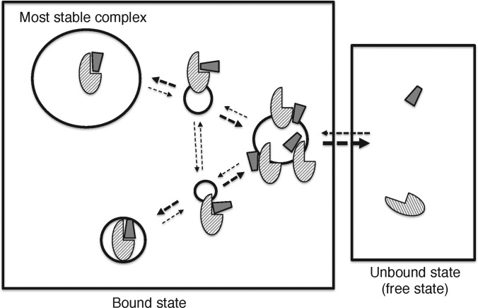
It is generally difficult to determine temporal complex structures in which the biomolecules are weakly interacting. Then an all-atom computer simulation such as molecular dynamics (MD) is a useful technique for quantifying those complex structures because the all-atom simulations can trace biomolecular motions at an atomic resolution at each moment of the complex formation. Figure 1 presents the processes of complex formation schematically, where semi-stable structural clusters are illustrated together with the most stable one. Imagine a simulation during which association and dissociation of molecules take place. The number of simulation snapshots assigned to a cluster relates to its stability (i.e. free energy): the more snapshots there are in a cluster, the lower the free energy assigned to it. The frequency of transitions from one cluster to another relates to the rate constant for the conformational change. Therefore, the simulation trajectory yields a diagram such as Figure 1.

Figure 1. Schematic representation of complex formation.

Solid-line circles represent populations of conformational clusters. Broken-line arrows represent possible pathways of conformational transitions. The larger the circle, the higher the population. The bolder the arrow, the larger the rate constant for the transition.

A quantitatively evaluated diagram is called a free-energy landscape; it provides key information for discussing the complex formation in detail. As it is difficult to obtain an ensemble of snapshots sufficient to generate the free-energy landscape using conventional sampling methods, several powerful computational methods have been developed. One way to approach the free-energy landscape is to use a powerful computer such as ANTON [3,4] or MDGRAPE [5] to perform simulation over a long period. The second way is to integrate many simulation trajectories, where the trajectories generate a wide conformational distribution [6] or rate constant among conformational clusters [7,8], although each trajectory may cover only a small fraction of the whole conformational space. The third way is to use a generalized ensemble method [9,10]. In the present review, we focus on various generalized ensemble methods that have been applied or are applicable to biomolecular binding with an atomic resolution in an explicit solvent to obtain the free-energy landscape. Table 1 lists the generalized ensemble methods that are introduced in the present review. We note that these methods are also applicable to large molecular conformational changes, such as protein folding or intramolecular conformational transitions, by changing the computation object.

Table 1. Variety of enhanced sampling methods.

Umbrella sampling type

Adaptive umbrella sampling

Adaptive lambda square dynamics

Metadynamics

Virtual system coupled adaptive umbrella MD Multicanonical MD

Multicanonical MD (every-run update)

Virtual system coupled multicanonical MD

Force-biased multicanonical MD (every-interval update)

Wang-Landau sampling (every-step update)

Simulated tempering type

Temperature replica exchange (parallel tempering)

Van der Waals radius exchange

Hamiltonian exchange

Coulomb exchange

Replica exchange with Suwa-Todo algorithm (non-detailed balance condition)

Other type

Double density dynamics

SAMPLING ENHANCEMENT BY GENERALIZED ENSEMBLE METHODS

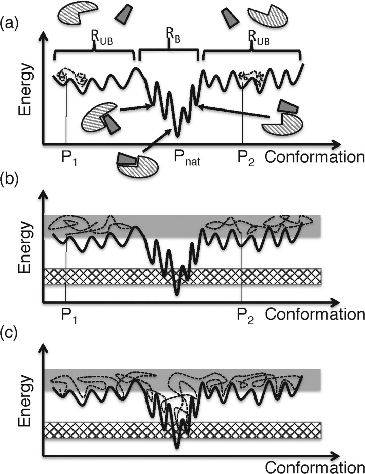
In computational biophysics, development of an effective conformational sampling method has been one of the central subjects. When force field parameters are assigned to constituent atoms of the system [protein(s), ligand(s) and solvents], the potential energy is computable to the protein system. In the present review, potential energy is simply called ‘energy’. Different conformations of the system have different energy. Therefore, an energy surface (Figure 2a) can in theory be constructed for the system. The problems are: the energy surface of the protein system has a large number of energy basins surrounded by energy barriers, and some of the conformational transitions among the basins are very slow processes. These difficulties arise as a result of the following factors: (i) the original conformational space is 3n-D for a system consisting of n atoms, and n is usually large; (ii) various types of interactions act among the constituent atoms; (iii) usually there is no structural symmetry in the system; and (iv) motions of an atom are influenced strongly by the surrounding atoms because they are densely packed.

Figure 2. Schematic representation of energy surface and simulation trajectories.

The x and y axes represent conformation and energy for a two-molecular system, respectively. The black curved line represents the energy surface, where energy minima and energy barriers are distributed. Although the conformation of the system is defined originally in a high-dimensional space, the space shown in this figure is one-dimensional (i.e. x axis). Molecular structures are also shown schematically. R_UB is a region where unbound or slightly touching molecules are distributed, and R_B a region where various complex forms are distributed. Although R_UB is divided into two in this figure, the two may be connected in the original high-dimensional space. (a) Broken lines represent simulation trajectories at room temperature starting from conformations at P₁ and P₂, which are far from the native complex structure (P_nat). The conformation moves slowly in the space because energy barriers interfere with the motion. (b) Simulation trajectories (broken lines) at high temperature. The trajectories fluctuate in a high-energy range (shaded energy range), which involves R_UB, and the room temperature range (checkered range) is not sampled. The volume of R_B is considerably narrower than that of R_UB in the original high-dimensional space. (c) Trajectory from multi-canonical simulation, which samples the high- and low-energy ranges evenly.

When performing a molecular simulation at room temperature (denoted as T_room), the conformation of the protein is usually trapped in energy basins near the initial conformation of the simulation (Figure 2a). Note that most proteins exert their biological functions at room temperature, and many biological experiments have been performed at this temperature. To sample a wide conformational area, overcoming energy barriers and reaching the native complex structure (i.e. experimentally determined complex structure at T_room), a long simulation is then needed when the simulation starts from a dissociated conformation. A simple method of sampling various conformations without being trapped is a high-temperature simulation (Figure 2b). This method, however, generates conformations accessible only at the high temperature. Inversely, when the high-temperature simulation starts from the native complex structure, this complex dissociates eventually, and the transition probability that the dissociated molecules rebind again to the native complex is negligibly small. A requirement imposed on the sampling method is that the resultant ensemble should consist of conformations that are probable at T_room in equilibrium (conformations in the checked energy range in Figure 2b), even when the simulation starts from a dissociated conformation. We denote this ensemble as Q(T_room). The free-energy landscape is derived from Q(T_room).

The high-dimensional space needed to express the protein conformation is beyond our comprehension. Then, contraction of the high-dimensional space into a low-dimensional space is essential. Some parameters, such as relative molecular orientation of one molecule to another, separation distance between two molecules or root mean square deviation from a reference complex structure, are useful for constructing the low-dimensional space for viewing the conformational distribution. Suppose that two parameters, denoted as s₁ and s₂, are selected for the coordinate axes of the contracted space (here it is a 2D space). Then a set of parameters [s₁,s₂] is calculated for all the conformations stored in Q(T_room), and a probability distribution function P_cano(s₁,s₂,T_room) is computed. A ‘potential of mean force’ (PMF), F(s₁,s₂,T_room), is formally defined as:

$$F(s_1,s_2,T_{\text{room}})=-R{T}_{\text{room}}\ln \left[P_{\text{cano}}(s_1,s_2,T_{\text{room}})\right]$$ 1

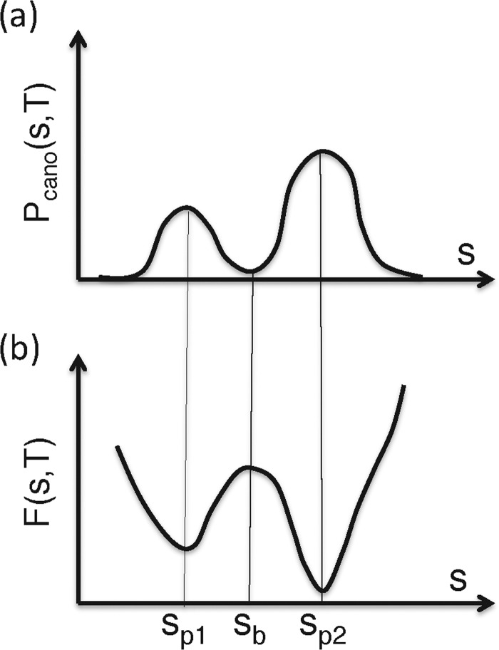
where R is the gas constant. Eqn 1 shows that a low PMF is assigned to a high-probability position. Note that high-probability regions in the conformational space are more stable thermodynamically than low-probability regions. In other words, the low-PMF regions are thermodynamically stable. Therefore, PMF is regarded as a free-energy landscape. The low-PMF regions are called ‘free-energy basins’, and the parameters s₁ and s₂ are called ‘reaction coordinates’. Figure 3 illustrates the relationship between P_cano and F in a 1D case. In a general case P_cano is converted as:

Figure 3. Conversion of distribution function to PMF in 1D case.

One-dimensional parameter is denoted as s. (a) Distribution P_cano (s, T), and (b) PMF F (s, T): F (s, T)=–RT [ln P_cano(s, T)]. High probability is assigned to S_p1 and S_p2, where F (s, T) is low. Contrarily, the low-probability is assigned to S_b, where F (s, T) is high.

$$\begin{array}{ccc}& & F(s_1,s_2,s_3,...,s_n,T_{\text{room}})\hfill \\ & & =-R{T}_{\text{room}}\ln \left[P_{\text{cano}}(s_1,s_2,s_3,...,s_n,T_{\text{room}})\right]\hfill \end{array}$$ 2

where both P_cano and F are expressed by n parameters.

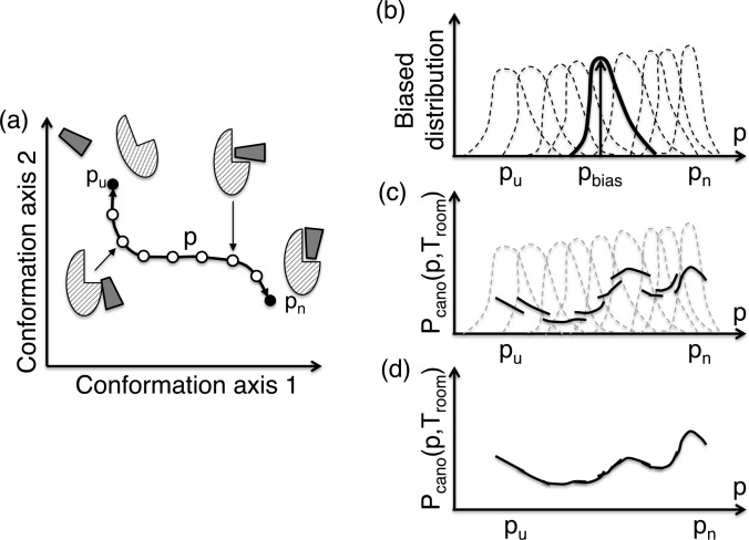
As an enhanced sampling method, we first introduce umbrella sampling [11,12]. In this method, an appropriate reaction coordinate p is set in advance so that the variation of p reflects the change of complex form well. Figure 4a shows the p axis schematically, which connects the unbound (P_u) and the native complex structures (P_n). The umbrella sampling method introduces bias functions known as ‘umbrella potential functions’ along the p axis. A bias potential set at a bias centre (one of the filled or open circles in Figure 4a) forces the conformation to be confined within a narrow region around the bias centre during a simulation. Then, performing individual simulations at different bias centres at temperature T_room, one can obtain a number of biased distribution functions (Figure 4b). The purpose of the umbrella sampling is to obtain an entire distribution function P_cano(p, T_room) without the effects of the biased potentials in the full range [P_u,P_n] of the p axis. Then a reweighting technique is applied to each of the biased distributions, and non-biased fragments of the entire distribution (Figure 4c) are obtained. Finally, smooth connection of the fragments produces P_cano(p, T_room) (Figure 4d). This connection technique is called a ‘weighted histogram analysis’ [13]. After the simulations, sampled snapshots are also reweighted and integrated into the conformational ensemble Q(T_room).

Figure 4. Scheme for explaining umbrella sampling.

(a) High-dimensional space is expressed here two-dimensionally (“conformation axis 1” and “conformation axis 2”), and reaction coordinate p is defined, for which the edges with filled circles labeled p_u and p_n correspond to unbound and native complex conformations, respectively. Open circles are intermediate conformations along the p-axis. (b) Biased distribution functions (broken and solid lines) obtained by individual simulations at different bias centers at temperature T_room. The solid line highlights a distribution around bias center pbias. (c) Solid lines are fragments of the full distribution function P_cano (p, T_room). Each fragment is computed only in well-sampled region of a biased distribution function in panel b. (d) P_cano (p, T_room) is obtained by smoothly connecting the fragments.

‘Adaptive umbrella sampling’ (AUS) [14,15] also introduces a bias function. However, this bias function is not for restricting the conformation in a narrow range of the reaction coordinate p. On the contrary, the bias assists the conformation to fluctuate smoothly in the range [P_u, P_n] (Figure 5a). In short, AUS is a method for enhancing the conformational fluctuations along the reaction coordinate. The bias potential E_AUS is given as:

Figure 5. Scheme for AUS.

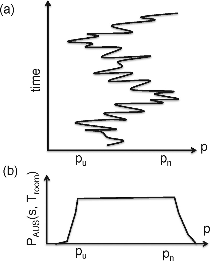
(a) The conformation fluctuates in range [p_u,p_n] of reaction–coordinate axis P with time. (b) Conformational distribution P_AUS(p, T_room) resulted from AUS.

$$E_{\text{AUS}}=E+R{T}_{\text{room}}\ln \left[P_{\text{cano}}(p,T_{\text{room}})\right]$$ 3

Note that the second term of the right-hand side of this equation is PMF (see eqns 1 and 2). An MD simulation at T_room, where E_AUS is used for evaluation of interatomic forces (force =−∇E_AUS), produces a flat distribution function P_cano(p, T_room) along the p axis (Figure 5b) when the function P_cano(p, T_room) is accurate enough and the simulation long enough: P_AUS(p, T_room) ≈ constant.

Note that the distribution function P_cano(p, T_room) is unknown in advance, and this function is then refined iteratively through simulations [10]. After a simulation has been finished, P_cano(p, T_room) is updated from the simulation trajectory and the next simulation is started using the updated function, etc. Through the iterations, P_AUS(p, T_room) is flattened more and more, and when P_AUS(p, T_room) becomes sufficiently flat, we judge that P_cano(p, T_room) is sufficiently accurate. Finally, we perform a long simulation using the refined P_cano(p, T_room) and store snapshots. Then Q (T_room) is generated, where a thermal weight at T_room is assigned to each of the stored snapshots (reweighting).

A method known as ‘metadynamics’ refines P_cano(p, T_room) within a simulation [16,17]. Thus, metadynamics is an iteration-free method and, therefore, suitable for automation of the simulation procedure [10]. Wang–Landau sampling [18], which enhances the conformational fluctuations along the energy axis as explained later, also refines a bias potential within a simulation.

Multi-canonical sampling was originally proposed for the study of the statistical properties of a physical model, the Potts model [19]. In this work, the Metropolis Monte Carlo algorithm was carried out to explore the conformational space. This method was then applied to biological systems [20–23], and extended to an MD scheme in which newtonian equations were solved in the cartesian coordinate space [24]. We denote this MD-based multi-canonical method as ‘McMD’. The adoption of the cartesian coordinates makes the sampling readily applicable to a multi-polypeptide system in an explicit solvent [25].

As with the AUS, multi-canonical sampling introduces an energy bias function (multi-canonical potential energy) as:

$$E_{\text{MC}}=E+R{T}_{\text{room}}\ln \left[P_{\text{cano}}(E,T_{\text{room}})\right]$$ 4

where P_cano(E,T_room) is the canonical energy distribution function at T_room. An MD simulation using atomic forces of force=-gradE_MC at T_room produces a flat distribution function P_MC(E, T_room)≈const along the energy axis when the function P_cano (E, T_room) is accurate enough and the simulation long enough. Therefore, the multi-canonical sampling enhances the fluctuations along the energy axis: when the system is in a high-energy range (the shaded range in Figure 2c), the conformation can overcome energy barriers, and when it is in a low-energy range (the chequered range in Figure 2c), which corresponds to the room temperature range, the sampled conformations are accumulated into the ensemble Q (T_room).

Recently, trajectory parallelization has been combined with McMD [6,26], and applied to a system consisting of a fragment taken from an intrinsically disordered protein (IDP) and its partner protein in an explicit solvent [27]. Furthermore, a virtual system, which has arbitrary physical properties defined by a researcher, has been introduced to enhance sampling and couple with the biomolecular system [28]. This procedure was named ‘virtual-system coupled multi-canonical molecular dynamics’ (V-McMD). The V-McMD method was combined with the trajectory parallelization and applied to the p53 interdomain linker, which is an intrinsically disordered region of p53 for regulating p53–DNA interactions [29].

As well as the AUS, the distribution function P_cano (E, T_room) is unknown in advance. This function is then determined iteratively: when the ith simulation run has been finished, P_cano(E, T_room) is updated using a recurrent equation (see Higo et al. [10]), E_MC is refined using eqn 4, and the (i+1)th run is performed. We call this procedure an ‘every-run’ update method. As mentioned above, the Wang–Landau sampling method [18] updates P_cano(E, T_room) at every step of the simulation. We call this updating method an ‘every-step’ update method. A force-biased McMD [30] is a method that is in between the every-run and every-step update methods: a long simulation can be regarded as a succession of simulation intervals (blocks). After a block has been finished, P_cano(E, T_room) is updated using the data in this block, and the simulation for the next block is started using the updated P_cano(E,T_room). We call this method an ‘every-interval’ update method, and it is also suitable for automating the simulation procedure.

Simulated tempering [31,32] is a method in which the temperature of the system changes as T₁→T₂→T₃→… during a simulation, satisfying the detailed balancing condition at temperature switching, and similar methods with simulated tempering have been proposed [33–35]. In this method, the temperature fluctuates, covering a range from T_room to high temperatures. When the temperature is elevated, the system overcomes energy barriers.

A method known as ‘temperature replica exchange method’ (tREM) [36,37] or ‘parallel tempering’ [38] introduces multiple systems (replicas), the chemical compositions of which are exactly the same, although the temperatures differ. These replicas evolve, according to the newtonian equations of motion (or Monte Carlo method) for a while, and occasionally exchange their temperatures, imposing the detailed balancing condition at exchange of temperature. Therefore, each replica experiences various temperatures during the time evolution. Importantly, replicas overcome energy barriers when their temperatures are high. One, at least, of the temperatures is set to T_room and, then, snapshots sampled at T_room are assembled in Q(T_room). Lyman et al. [39] expanded the replica exchange method in which replicas are expressed by different resolution models, such as all-atom and coarse-grained models, and the resolutions are exchanged among the replicas in a simulation. In fact, the quantity to be exchanged is arbitrary [40]; some exchange methods have been proposed: exchange of van der Waals’ radius [41], coulomb interactions [42] and hamiltonian (i.e. Hamiltonian exchange) [43].

A method called ‘λ dynamics’ [44,45] also enhances the conformational fluctuations along an arbitrary structural parameter (the reaction coordinate called λ), as with AUS. In λ dynamics, however, the reaction coordinate is treated as a dynamic quantity, i.e. λ, and its momentum, p_λ, is involved as a dynamic variable in equations of motion. Ikebe et al. [46] recently proposed an extended form of λ dynamics, adaptive λ square dynamics (ALSD), in which different weights are assigned to each energy term and the weights fluctuate as dynamic variables. ALSD is effective for sampling a biomolecular system in which very strong and weak interactions are mixed [47].

In most of conformational sampling methods based on the Monte Carlo scheme, the conformational changes are controlled by the detailed balancing condition. Recently, an algorithm, called the Suwa–Todo algorithm [48], has been proposed based on a balancing condition (non-detailed balancing condition). Probability fluxes may then occur in time evolution of the system's probability distribution function. Importantly, an equilibrated distribution is obtained finally in spite of the fact that the detailed balance condition is broken. Based on the Suwa–Todo algorithm, biomolecular sampling methods have been proposed [49,50], in which, although the method has a similar fashion to the replica exchange method, the exchange (or permutation) rule among the replicas obeys the Suwa–Todo condition. These methods may generate a new trend in conformational sampling.

Double density dynamics (DDD) is a sampling method in which an arbitrary parameter and its momentum are treated as dynamic variables in the equations of motion [51]. As a result, the parameter fluctuates in a given range. One may think that DDD is similar to the λ dynamics or ALSD mentioned above. In DDD, however, the statistics that microscopic states obey can be designed arbitrarily. Thus, one can optimize the sampling efficiency by modulating the statistics in theory.

SEMI-STABLE CONFORMATIONAL CLUSTERS IN AN IDP SYSTEM

We mentioned in the Introduction that the generalized ensemble method elucidates not only the most thermodynamically stable state (the largest conformational cluster), but also semi-stable states, which may appear temporally in the molecular binding process. In the present review we introduce our recent computational study on an IDP interacting with its partner protein. IDP is a challenging system for examining the efficiency of the generalized ensemble methods because IDPs have larger conformational fluctuations than ordered proteins (regular proteins). Therefore, the free-energy landscape of an IDP consists of both the most stable and the semi-stable states.

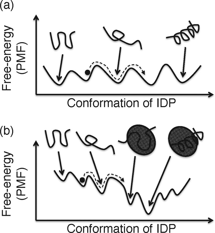
An ordered protein has its own tertiary structure (native structure) determined by its amino acid sequence, which does not vary largely before and after complex formation. A unique tertiary structure is not assigned to the IDP when the IDP is in the unbound (isolated) state, and the unique structure is formed when it binds to its partner molecules [52–54]. This mechanism is known as ‘coupled folding and binding’ [54]. Therefore, the free-energy landscape of an IDP in the unbound state has no dominant cluster prevailing against the other clusters (Figure 6a). In the bound state, on the contrary, the landscape has the dominant cluster (the most stable complex) (Figure 6b).

Figure 6. Schematic free-energy landscape of IDP.

(a) Unbound and (b) bound states shown one-dimensionally. The x axis represents the conformation of IDP, although the system in (b) consists of two molecules (IDP and its partner). The black filled circle represents the IDP conformation moving along a simulation trajectory (broken line).

We have computed the free-energy landscape of two systems: NRSF–mSin3 [27] and pKID–KIX [55] systems, in which NRSF and pKID are IDPs, and mSin2 and KIX their partner proteins. In the present review, we focus on the NRSF–mSin3 system. NRSF (the N-terminal repressor domain of neural restrictive silencer factor) is an IDP known to be an essential transcriptional repressor for neuron-specific genes in non-neuronal cells and neuronal progenitors, and mSin3 is its partner protein. The complex structure was solved using NMR [56]: a 15-residue segment of a NRSF fragment folded into a helix when bound to the cleft on the surface of the paired amphipathic helix (PAH) domain of mSin3. The regions of NRSF other than the 15-residue segment are disordered even in the complex structure.

In the McMD simulation, the 15-residue fragment and the PAH domain of mSin3 were treated. We denote the PAH domain of mSin3 simply as mSin3. In the initial conformation of the simulation, these two molecules were distant from each other in an explicit solvent. Furthermore, the conformation of the NRSF segment was disordered in advance (Figure 1c in Higo et al. [27]). After refinement of the multi-canonical energy E_MC (eqn 4) via iterative McMD simulations, the production runs were performed yielding the ensemble Q(300K). McMD of the single NRSF fragment (i.e. unbound state) was also performed with a similar simulation procedure. The initial conformation of the NRSF fragment was randomized in advance and put in an explicit solvent (Figure 1b in Higo et al. [27]).

Conformational clustering applied to Q(300K) has shown that the largest cluster (i.e. the most stable cluster) is the native-like complex cluster (Figure 7 in Higo et al. [27]). Thus, the McMD simulations provided reliable data, in the sense that the NMR complex was predicted correctly. In a high-energy range, the NRSF fragment distributed widely in space without a dominant structure (Figure 4A in Higo et al. [27]). On the other hand, at 300K, the NRSF segment was trapped into the NRSF-binding cleft of mSin3 (Figure 4B in Higo et al. [27]). Figure 7 demonstrates the conformational distribution for Q(300K) projected in an abstract conformational space. Note that a region with crowded dots (conformations) corresponds to a low free-energy (PMF) region (see eqn 2). Figure 7 shows that three domains of crowded dots exist and that the domains were spaced by broken lines labelled b₁ and b₂, along which the dots distribute sparsely. These sparsely dotted regions correspond to free-energy barriers because the probability of conformation around the regions is low. The domains were discriminated well by the molecular orientation of the NRSF fragment in the NRSF-binding cleft of mSin3 (see Figure 7). Therefore the rearrangement of the molecular orientation of the fragment requires jumping over the free-energy barriers.

Figure 7. Conformational distribution of Q(300K) for system consisting of the NRSF fragment and mSin3.

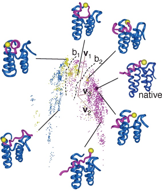
(a) The distribution is shown in an abstract 3D space, with coordinate axes (orange–tan coloured lines) labelled v₁, v₂ and v₃, which are calculated using principal component analysis: each coloured dot is a projection of a conformation of the NRSF fragment in the 3D space (see Higo et al. [27]). The closer the two dots, the more similar the two conformations. Some tertiary structures are also displayed, in which the magenta model is the NRSF fragment and the blue model mSin3. Yellow spheres indicate the N-terminus of the NRSF fragment. The black sphere represents the position of the NMR complex structure labelled ‘native’. There are three large domains spaced by broken lines labelled b₁ and b₂, along which dots distribute sparsely. Dots are coloured depending on mutual molecular orientations between the two molecules: the colour is magenta when the NRSF fragment is approximately parallel to the cleft of mSin3 and cyan when they are approximately anti-parallel. Otherwise, the colour is yellow. See Higo et al. [27] for strict colouring method.

Figure 8 represents the conformational distribution of Q(300K) for the single NRSF fragment. A variety of conformations, such as helix, hairpin or bent, are seen in the conformational space, which means that the conformation fluctuates among these structures in solution at 300K: no dominant structure exists. Therefore, the NRSF fragment is disordered in the unbound state. It is interesting that most of the conformations in Q(300K) of the single NRSF system are found in the NRSF–mSin3 system, whereas the probabilities assigned to the conformations are different between the two systems (Figure 10 in Higo et al. [27]). The main feature for the complex state was a helix, although the single NRSF fragment adopts both the helix and the hairpin (Figure 3 in Higo et al. [27]).

Figure 8. Conformational distribution of Q(300 K) for single NRSF fragment.

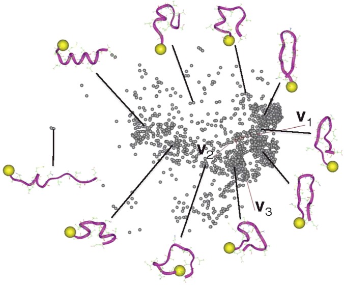
Axes v₁, v₂ and v₃ are calculated as for Figure 7. Some conformations are also displayed. Yellow spheres indicate the N-terminus of the NRSF fragment.

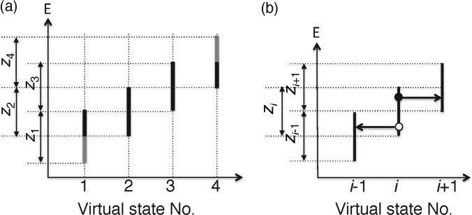
Figure 10. Space constructed by the energy axis and virtual-state axis, where four virtual states exist as an example.

(a) Although the widths of the zones are shown equally in this figure, they are not necessarily the same in the actual sampling. (b) Transitions among adjacent virtual states (see text).

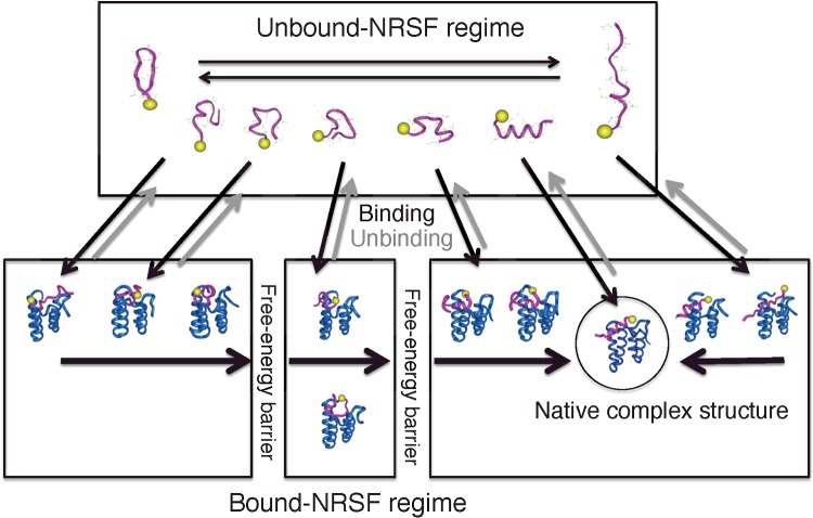
From these results, we proposed a mechanism for the coupled folding and binding of NRSF (Figure 9): in the unbound regimen, NRSF fluctuates among various conformations. NRSF binds with the cleft of mSin3 when using these conformations, and non-native complexes are formed. The NRSF conformation moves in the bound regime. Otherwise the complex dissociates. Depending on the first formed non-native complex, the complex may overcome one or two free-energy barriers, and finally the native complex is formed. The McMD simulation has shown that the complex formation with the all-atom model is considerably complicated where the complex experiences various intermediates overcoming free-energy barriers.

Figure 9. Simplified free-energy landscape integrated from the all-atom detailed free-energy landscapes for the NRSF–mSim3 complex and single-chain NRSF.

Arrows represent conformational changes. Yellow spheres in the molecular models indicate the N-terminus of the NRSF fragment.

VIRTUAL-SYSTEM COUPLING

Above we introduced various enhanced conformational sampling methods. Now we introduce a ‘virtual system’, which couples with the biomolecular system (a ‘real system’) [57]. The entire system is the sum of the real and the virtual systems, which are specified by the coordinates x for the real system (i.e. coordinates of the constituent atoms of the molecular system) and a state parameter for the virtual system. In a simulation, both the real and virtual systems move. Advantageously, one can set the virtual system arbitrarily. We trace the time development of the entire system rather than pursuing just the motions of the real system. Recently, the virtual system was integrated with McMD and AUS, abbreviated as ‘V-McMD’ [28] and ‘V-AUS’ [58], respectively. Although it may be difficult to understand the coupling between the real and virtual systems intuitively, the computational technique is simple as explained below (see Higo et al. [28] for details).

Imagine a virtual system, for which the state is specified by a discrete ordinal number i (‘virtual-state index’). We assume that when the virtual-state index is i, the energy of the real system E(x) is confined in an energy zone z_i as: z_i=[E^min_i] ⩽ E ⩽ E^max_i]. Figure 10a represents a space constructed by the energy axis and virtual-state axis. Zones z_i−1 and z_i (e.g. z₁ and z₂) overlap each other as well as z_i and z_i+1 (e.g. z₂ and z₃) do, but two zones, z_i−1 and z_i+1, do not overlap because they are set as: E^min_i+1 − E_{i − 1}^max > ε, where ε is a positive but infinitely small number. In time development of the entire system, the conformation of the real system varies according to the equations of motion, and the virtual-state index jumps i to i+1 or i−1, which causes the variable energy range for the real system to be reset. If inter-virtual state transitions are exhibited in the simulation, the real system fluctuates within z_i, which means that only a narrow region of the conformational space is sampled (i.e. sampling efficiency is low).

We define the inter-virtual state transitions as follows: suppose that E is at the filled-circle position in Figure 10b. Then, the virtual state i may jump to the virtual state i+1 without changing x of the real system. On the other hand, if E is at the open-circle position, the virtual state may move to i−1. At this point, we introduce a rule: during a time interval of [t, t+τ], the virtual state number is fixed to i, and x moves according to the ordinary equations of motion confining E in z_i. At time t+τ the transition to z_i−1 or z_i+1 is achieved with transition probability ρ_t (0≤ρ_t≤1), at which x does not move. Due to the arbitrary property of the virtual system, one can set the transition probability ρ_t and the interval τ, arbitrarily, which may increase the sampling efficiency [28,57]. Consequently, by travelling the virtual states, the real system fluctuates across the wide conformational space overcoming energy barriers. The detailed balance for this time development is theoretically well satisfied, as described in the Appendix. Introduction of the virtual system to AUS is explained in Higo et al. [58].

Recently, Moritsugu et al. [59,60] introduced ‘multiscale essential sampling’ (MSES), in which a protein system was expressed by an all-atom model, coupled with a coarse-grained model(s) to enhance conformational sampling. MSES was applied to protein–protein binding of a barnase–barstar system [61]. The free-energy landscape for association/dissociation demonstrated the existence of the non-native complex forms as well as the native complex. Although the methodological fashion of MSES is considerably different from the virtual-system coupling method, the two methods have a similarity in introducing non-realistic systems for coupling with the real system.

FREE-ENERGY LANDSCAPE FOR DIMER FORMATION BY V-McMD

In the present review, as an example of a generalized ensemble method applied to a biomolecular complex formation, we show the free-energy landscape of homo-dimer formation of an endothelin-1 (ET1) derivative computed by V-McMD simulations. ET1 is a biomolecule of 21 amino acids, known as a strong vasoconstrictor of a vessel's smooth muscles [62–64]. This molecule is a potent drug target because it is related to many human diseases [65–69]. The tertiary structure was solved by NMR spectroscopy [70–72] and X-ray crystallography [73]. In either study, the N-terminal region adopts a strand and the middle region forms an α-helix. As two disulfide bonds link the strand and the helix, the tertiary structure is compact and stable regardless of its short polypeptide length.

ET1 aggregates at a concentration of 1–4 mM. To increase the solubility, the N-terminus was then extended by two charged amino acid residues, lysine and arginine [74], which exist in its precursor protein. This extended ET1 is denoted as KR-ET1. Unexpectedly and of interest, KR-ET1 has less activity than ET1 in spite of an increase in solubility. Then, X-ray crystallography [75] showed that KR-ET1 forms a homo-dimer (PDBID; 1t7h) (Figure 11a), in which the orientations of the two molecules are anti-parallel to each other, although the molecular tertiary structure is similar to that of the single ET1 structure. In this study, five amino acid residues at the C-terminus of KR-ET1 were removed because those residues are presumably disordered and exposed in solution. This truncated peptide of 18 amino acids (sequence: KRCSCSSLMDKECVYFCH) is denoted as KR-CSH-ET1. Figure 11a indicates that this complex is stabilized by three factors: intermolecular β-sheet, intermolecular hydrophobic stacking of phenylalanine side-chain rings and two intermolecular salt bridges. Therefore, the experimental study of Hoh et al. [75] reported that this homo-dimer structure has considerable stability.

Figure 11. Homo-dimer complex of KR-CSH-ET1 determined by X-ray crystallography.

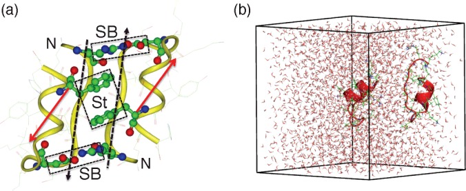
(a) Two ‘N’ characters indicate the N-termini of the molecules. An intermolecular β-sheet is formed between two strands indicated by black broken-line arrows. Intermolecular hydrophobic stacking between phenylalanine side-chain rings is shown by the rectangle labelled ‘St’. Two intermolecular salt bridges, formed between arginine and aspartic acid, are indicated by the rectangles labelled ‘SB’. Red arrows are used to identify the molecular orientations of the two molecules, which point from the Cα atom of lysine to the Cα atom of the last cysteine in the sequence KR-CSH-ET1. (b) Initial conformation of V-McMD simulation.

The dimer formation of KR-CSH-ET1 is an appropriate target for assessing V-McMD because the complex form is discriminated well by two quantities: the mutual molecular orientation, , and the intermolecular separation distance, r₁₂, the exact definition of which is given later. Previously we performed V-McMD simulations for KR-CSH-ET1 dimer formation [28], where the two molecules were confined in a spherical droplet of an explicit solvent, and the 2D free-energy landscape was computed. The free-energy landscape at room temperature was predominantly composed of the crystallographic native complex structure. In the present review, we performed V-McMD of the KR-CSH-ET1 dimer formation with a periodic boundary condition, and computed the free-energy landscape.

The simulation system was generated as follows: one KR-CSH-ET1 was immersed at the centre of a periodic box (box size: 45³ Å³; 1 Å=0.1 nm) filled by an explicit solvent; the other KR-CSH-ET1 was put at a position apart from the first molecule. The system consisted of 8706 atoms (580 atoms for the KR-CSH-ET1 molecules, 9 Na⁺, 11 Cl⁻ ions and 2702 water molecules). The number of ions was determined to set the solution at a physiological salt concentration. Then a constant-pressure MD simulation was performed at room temperature and pressure of 1.0 atm, by which the initial conformation for V-McMD was prepared (resultant box size: 44.003683 Å³) (Figure 11b). The V-McMD simulation procedure was similar to that for the previous study [28] as follows: first refinement of E_MC was done via iterative V-McMD simulations, and then a V-McMD simulation was performed to produce an entire conformational ensemble. The conformational ensemble Q(T_room) was constructed by reweighting the snapshots in the entire ensemble.

In V-McMD the energy moves in a wide range as mentioned previously. KR-CSH-ET1 may then unfold when the system is elevated to a high-energy region. The purpose of the present review is to show the free-energy landscape for the molecular binding, and refolding of KR-CSH-ET1 is outside its scope. Thus, we restrained the tertiary structure of each KR-CSH-ET1 weakly by intramolecular restraint functions (see Higo et al. [28] for technical details). Thus, the translational and rotational motions of the KR-CSH-ET1 molecules were free to maintain their tertiary structures.

In the present review, we set T_room as 310K and obtained a canonical ensemble Q(310K). Figure 12(a) demonstrates a free-energy landscape at 310K, presented in 2D by , and r₁₂, the exact definition of which is given in Figure 12(a). From Figure 12(a), the largest cluster (i.e. the lowest free-energy cluster) is native like, whereas the two KR-CSH-ET1 molecules are arranged anti-parallel and the three factors, mentioned above, stabilized the complex structure. We call this cluster the native-like cluster. The landscape provided two other clusters: in the second largest cluster (the second lowest free-energy cluster), the orientations of the two KR-CSH-ET1 molecules are approximately perpendicular to each other: ≈ 0 The third largest cluster (the third lowest free-energy cluster) was characterized by ≈ 1, which means that the relative orientations of the two molecules are parallel. In the solvent–droplet boundary condition [28], the free-energy landscape had only the native-like cluster. It is likely that the solvent–droplet boundary condition would result in a stronger pressure than 1 atm in the droplet centre due to the surface tension of the spherical droplet. This strong pressure could stabilize the well-packed conformation (i.e. native complex), and then probabilities assigned to the non-native complexes were diminished. The periodic boundary condition does not induce such an artificial excess pressure because there is no free surface in this treatment.

Figure 12. Free-energy landscapes.

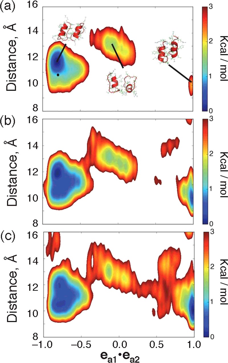
Free-energy landscapes at (a) 310 K, (b) 350 K, and (c) 370 K. x-axis is mutual molecular orientation, which is a scalar product of e_a1 and e_a2, where e_a1 and e_a2 are unit vectors parallel to the red-colored vectors defined in Figure 11a: . Orientations of two KR-CSH-ET1 molecules are approximately parallel, anti-parallel, and perpendicular to each other for , and respectively. y-axis is inter-molecular separation distance r₁₂=| r_G1−r_G2 | where r_G1 and r_G2 are positions of the geometrical centres of the two molecules, and the geometrical centre is computed from the Cα-atomic positions of each molecule. The free-energy value (PMF; Eq. 1), whose height is shown by the coloured scale bars, is set so that the lowest PMF is zero. Tertiary structures from three clusters at 300 K are shown in panel (a), where the small black filled circle indicates the position of the native complex experimentally determined.

Figures 12(b) and 12(c) demonstrate free-energy landscapes at 350K and 370K, respectively. The largest and second largest clusters are connected at 350K, although the third largest cluster is still isolated. At 370K, the third largest cluster is connected to the second largest cluster. We presume that, once a non-native complex is formed in the cluster of ≈ 0, this complex can transition to the native-like cluster relatively readily. On the other hand, once a non-native complex has been formed in the cluster of ≈ 1, this complex should overcome a high-energy barrier to reach the native-like cluster via the cluster of ≈ 0. Otherwise, this complex dissociates, and the free KR-CSH-ET1 molecules may reassociate after that. Another interesting result from Figure 12 is that the second largest cluster at 300K and 350K is the third largest cluster at 370K.

We exemplify, in this section, that the generalized ensemble method is a powerful tool to compute the free-energy landscape, through which we can discuss the thermodynamic stability of the clusters, the cluster networks and the temperature dependence of the networks.

CONCLUSION

In the present review, we have introduced various generalized ensemble methods, focusing in particular on methods applicable to biomolecular association/dissociation with an atomic resolution in explicit solvent to obtain the free-energy landscape. To make the methods useful for drug discovery, the methods should not only explain basic mechanisms for association/dissociation, but also predict the complex forms and their stabilities. From this point of view, the sampling methods are useful if they generate a free-energy landscape for complex formation in explicit solvent at atomic resolution. In the Introduction, we listed three approaches: fast computations, multiple simulation runs and generalized ensemble methods. Note that these approaches can be combined, e.g. trajectory parallelization has been used for multi-canonical sampling and AUS. The free-energy landscape obtained from the generalized ensemble method does not involve information on rate constants. However, from knowledge about the locations of many locally stable states, it is possible to look for the shortest path between a pair of conformational clusters, e.g. using the string method [76], and the activation energy overcoming the energy barrier can be computed. In addition, combination of the generalized ensemble methods with the rate-constant estimation method, using the Markov state model [7,8] among conformational clusters, may be useful.

In living matter, a number of biological molecules (proteins, metabolites and DNAs) crowd together in solution (water and ions). Recent studies reveal that crowding itself provides and/or enhances the biomolecules’ activities [77,78]. These large-scale studies, however, view the biomolecules, neglecting their atomic details. Therefore, detailed intermolecular information from the generalized ensemble methods is useful to complete the molecular picture for living matter.

Most MD simulations in current use are based on classical mechanics (newtonian dynamics). On the other hand, many important processes taking place in living matter, such as catalytic reactions, are quantum chemical. Thus, development of quantum-mechanical MD [79–83] is an important step for elucidating vividly biochemical reactions in living matter, although there is a way to go before being applied to large biomolecular systems. One of the goals of the generalized ensemble methods is to be coupled with the quantum-mechanical technique in the molecular crowding environment.

Abbreviations

ALSD

adaptive λ square dynamics

AUS

adaptive umbrella sampling

DDD

double density dynamics

ET1

endothelin-1

IDP

intrinsically disordered protein

McMD

MD-based multi-canonical method

MD

molecular dynamics

MSES

multiscale essential sampling

NRSF

N-terminal repressor domain of neural restrictive silencer factor

PAH

paired amphipathic helix

PMF

potential of mean force

APPENDIX

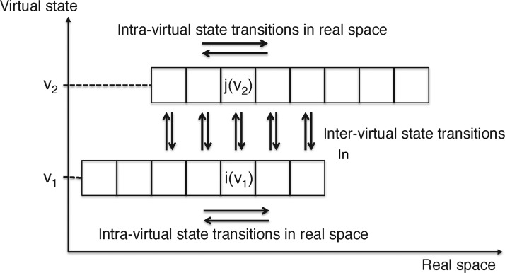
As explained in the main text, the virtual-system coupling method allows two types of variations for the entire system (molecular system plus virtual system): the biomolecular conformational variations in real space and the virtual-state index variations. In this appendix, we show that these variations satisfy the detailed balance. We simplify the system as illustrated in Figure 13, which does not negate the generality of the discussion. In Figure 13, there are only two virtual states (index v_m; m=1,2) and the real space is divided into small bins to specify the site positions. Each site is denoted by i(v_m), where i is the site ordinal number in a virtual state v_m. The biomolecular conformational variations are intra-virtual state transitions shown by horizontal arrows in Figure 13, and the virtual-state index variations are inter-virtual state transitions shown by the vertical arrows. The probability assigned at i(v_m) is denoted as ρ_i(vm)(t), where t is time.

Figure 13. Scheme for explaining detailed-balance satisfaction in the virtual-system coupling method.

Time development of ρ_i(vm)(t) by the intra-virtual state transi-tions is expressed formally as:

$${\rho }_{i\left(v_m\right)}(t+\Delta \tau )=\sum _k^{k\in v_m}{a}_{k\left(v_m\right)\to i\left(v_m\right)}{\rho }_{k\left(v_m\right)}\left(t\right),$$ 5

where a_{k(vm)→i(vm)} is the transition probability from k(v_m) to i(v_m) during Δτ. Then the term a_{k(vm) → i(vm)}ρ_k(vm)(t) is the probability flux from k(v_m) to i(v_m) during Δτ. Summation of the stay probability in i(v_m) and the outflux probabilities from i(v_m) is unity:

$$\sum _k^{k\in v_m}{a}_{i\left(v_m\right)\to k\left(v_m\right)}=1(\forall i)$$ 6

Then, eqn 5 is rewritten using eqn 6 as:

$${\rho }_{i\left(v_m\right)}(t+\Delta \tau )={\rho }_{i\left(v_m\right)}\left(t\right)+\Delta {\rho }_{i\left(v_m\right)},$$ 7

where:

$$\begin{array}{ccc}\hfill \Delta {\rho }_{i\left(v_m\right)}& =& \sum _{k(\ne i)}^{k\in v_m}\left[a_{k\left(v_m\right)\to i\left(v_m\right)}{\rho }_{k\left(v_m\right)}\left(t\right)-a_{i\left(v_m\right)\to k\left(v_m\right)}{\rho }_{i\left(v_m\right)}\left(t\right)\right]\hfill \\ & =& \sum _{k(\ne i)}^{k\in v_m}\Delta A_k.\hfill \end{array}$$ 8

Eqn 7 is applied to all the sites in each virtual state, and further time development is achieved by repeating this procedure M times: ρ_i(vm)(t)→ρ_i(vm)(t′), where t′=MΔτ.

Next, we consider the inter-virtual state transitions. Suppose that two sites, i(v₁) and j(v₂) belong to different virtual states and are connected by vertical arrows as in Figure 13. Then, variation of ρ_i(v1)(t′)ρ_j(v2)(t′) by the inter-virtual state transition is:

$$\left\{\begin{array}{c}\rho {}_{i\left(v_1\right)}^{*}\left(t^{\prime }\right)=b_{i\left(v_1\right)\to i\left(v_1\right)}{\rho }_{i\left(v_1\right)}\left(t^{\prime }\right)+b_{j\left(v_2\right)\to i\left(v_1\right)}{\rho }_{j\left(v_2\right)}\left(t^{\prime }\right)\hfill \\ \rho {}_{j\left(v_2\right)}^{*}\left(t^{\prime }\right)=b_{i\left(v_1\right)\to j\left(v_2\right)}{\rho }_{i\left(v_1\right)}\left(t^{\prime }\right)+b_{j\left(v_2\right)\to j\left(v_2\right)}{\rho }_{j\left(v_2\right)}\left(t^{\prime }\right),\hfill \end{array}\right.$$ 9

where b_{i(v1) → j(v2)} and b_{j(v2) → i(v1)} are the inter-virtual state transition probabilities from i(v₁) to j(v₂) and from j(v₂) to i(v₁) respectively. Two quantities, b_{i(v1) → i(v1)} and b_{j(v2) → j(v2)}, are the stay probabilities in i(v₁) to j(v₂), respectively. The probability invariants are given as:

$$\left\{\begin{array}{c}{b}_{i\left(v_1\right)\to i\left(v_1\right)}+b_{i\left(v_1\right)\to j\left(v_2\right)}=1\hfill \\ b_{j\left(v_2\right)\to i\left(v_1\right)}+b_{j\left(v_2\right)\to j\left(v_2\right)}=1\hfill \end{array}\right.$$ 10

Using the invariants, eqn 9 is rewritten as:

$$\left\{\begin{array}{c}\rho {}_{i\left(v_1\right)}^{*}\left(t^{\prime }\right)={\rho }_{i\left(v_1\right)}\left(t^{\prime }\right)+\Delta \rho {}_{i\left(v_1\right)}^{*}\hfill \\ \rho {}_{j\left(v_2\right)}^{*}\left(t^{\prime }\right)={\rho }_{j\left(v_2\right)}\left(t^{\prime }\right)+\Delta \rho {}_{j\left(v_2\right)}^{*}\hfill \end{array}\right.$$ 11

where

$$\left\{\begin{array}{c}\Delta \rho {}_{i\left(v_1\right)}^{*}=b_{j\left(v_2\right)\to i\left(v_1\right)}{\rho }_{j\left(v_2\right)}\left(t^{\prime }\right)-b_{i\left(v_1\right)\to j\left(v_2\right)}{\rho }_{i\left(v_1\right)}\left(t^{\prime }\right)\hfill \\ \Delta \rho {}_{j\left(v_2\right)}^{*}=b_{i\left(v_1\right)\to j\left(v_2\right)}{\rho }_{i\left(v_1\right)}\left(t^{\prime }\right)-b_{j\left(v_2\right)\to i\left(v_1\right)}{\rho }_{j\left(v_2\right)}\left(t^{\prime }\right)\hfill \end{array}\right.$$ 12

The asterisks in eqns 9, 11 and 12 are introduced to indicate clearly that time t′ does not evolve by the inter-virtual state transitions because the real system does not move with these transitions. Eqn 11 is applied to all sites that are connected by vertical arrows in Figure 13.

In the virtual-system coupling method, the variation ρ_i(vm)(t) → ρ*_i(vm)(t+MΔτ) is achieved by repeating eqn 7 M times followed by eqn 11. Repetition of this procedure yields a stationary state as:

$$\begin{array}{ccc}\hfill {\rho }_{i\left(v_m\right)}\left(t\right)& \to & \rho {}_{i\left(v_m\right)}^{*}\left(t+M\Delta \tau \right)\to \rho {}_{i\left(v_m\right)}^{*}\left(t+2M\Delta \tau \right)\hfill \\ & \to & ...\to {\rho }_{i\left(v_m\right)}\left(\infty \right).\hfill \end{array}$$

Below we determine the stationary state. First, remember that V-McMD or V-AUS is designed so that probabilities converge to a constant for each virtual state:

$${\rho }_{i\left(v_m\right)}\left(\infty \right)=c_m(m=1,2)$$ 13

where the two constants c₁ and c₂ are not necessarily the same because eqn 7 does not involve the inter-virtual state transitions. Eqn 13 is equivalent to the following equation:

$$a_{k\left(v_m\right)\to i\left(v_m\right)}^{}=a_{i\left(v_m\right)\to k\left(v_m\right)}^{}$$ 14

where (m=1, 2). Next, remember that the inter-virtual state transition probabilities in V-McMD or V-AUS are set as:

$$b_{j\left(v_{m^{\prime }}\right)\to i\left(v_m\right)}=b_{i\left(v_m\right)\to j\left(v_{m^{\prime }}\right)}=1$$ 15

where m=m′.

Then, we define the following probabilities:

$${\rho }_{i\left(v_1\right)}={\rho }_{j\left(v_2\right)}=\mathit{c}onst(\forall i\mathrm{and}\forall j)$$ 16

From eqns 14 and 15, the set of probabilities defined by eqn 16 satisfies the following equations:

$$\begin{array}{c}\left\{\begin{array}{c}\Delta A_k=0\hfill \\ \Delta \rho {}^{*}{}_{i\left(v_m\right)}=0\hfill \end{array}\right.\hfill \end{array}$$ 17

Therefore, eqn 16 defines the stationary state and eqn 17 shows that the detailed balance is satisfied (i.e. the stationary state is the equilibrium state).

In the above discussion, M was constant. However, M can vary arbitrarily in the sampling to reach the same equilibrium state (eqn 16). Besides, the discussion above does not alter for other systems with many more virtual states and an infinitely small bin size.

FUNDING

J. Higo was supported by a Grant-in-Aid for Scientific Research on Innovative Areas [21113006] received from the Ministry of Education, Culture, Sports, Science and Technology (MEXT), Japan and by the development of core technologies for innovative drug development based on IT from the Japan Agency for Medical Research and Development (AMED); S. Iida and H. Nakamura were supported by the Japan Society for the Promotion of Science KAKENHI, Grant-in-Aid for Scientific Research on Innovative Areas [grant number 24118001].

References

- 1.Li Y., Lipschultz C.A., Mohan S., Smith-Gill S.J. Mutations of an epitope hot-spot residue alter rate limiting steps of antigen–antibody protein–protein associations. Biochemistry. 2001;40:2011–2022. doi: 10.1021/bi0014148. [DOI] [PubMed] [Google Scholar]
- 2.Tompa P., Fuxreiter M. Fuzzy complexes: polymorphism and structural disorder in protein-protein interactions. Trends Biochem. Sci. 2008;33:2–8. doi: 10.1016/j.tibs.2007.10.003. [DOI] [PubMed] [Google Scholar]
- 3.Lindorff-Larsen K., Piana S., Dror R.O., Shaw D.E. How fast-folding proteins fold. Science. 2011;334:517–520. doi: 10.1126/science.1208351. [DOI] [PubMed] [Google Scholar]
- 4.Shan Y., Gnanasambandan K., Ungureanu D., Kim E.T., Hammarén H., Yamashita K., Silvennoinen O., Shaw D.E., Hubbard S.R. Molecular basis for pseudokinase-dependent autoinhibition of JAK2 tyrosine kinase. Nat. Struct. Mol. Biol. 2014;21:579–584. doi: 10.1038/nsmb.2849. [DOI] [PMC free article] [PubMed] [Google Scholar]
- 5.Kikugawa G., Apostolov R., Kamiya N., Taiji M., Himeno R., Nakamura H., Yonezawa Y. Application of MDGRAPE-3, a special purpose board for molecular dynamics simulations, to periodic biomolecular systems. J. Comput. Chem. 2009;30:110–118. doi: 10.1002/jcc.21035. [DOI] [PubMed] [Google Scholar]
- 6.Ikebe J., Umezawa K., Kamiya N., Sugihara T., Yonezawa Y., Takano Y., Nakamura H., Higo J. Theory for trivial trajectory parallelization of multicanonical molecular dynamics and application to a polypeptide in water. J. Comput. Chem. 2011;32:1286–1297. doi: 10.1002/jcc.21710. [DOI] [PubMed] [Google Scholar]
- 7.Lane T.J., Shukla D., Beauchamp K.A., Pande V. S. To milliseconds and beyond: challenges in the simulation of protein folding. Curr. Opin. Struct. Biol. 2013;23:58–65. doi: 10.1016/j.sbi.2012.11.002. [DOI] [PMC free article] [PubMed] [Google Scholar]
- 8.Chodera J.D., Noé F. Markov state models of biomolecular conformational dynamics. Curr. Opin. Struct. Biol. 2014;25:135–144. doi: 10.1016/j.sbi.2014.04.002. [DOI] [PMC free article] [PubMed] [Google Scholar]
- 9.Mitsutake A., Sugita Y., Okamoto Y. Generalized-ensemble algorithms for molecular simulations of biopolymers. Biopolymers. 2001;60:96–123. doi: 10.1002/1097-0282(2001)60:2<96::AID-BIP1007>3.0.CO;2-F. [DOI] [PubMed] [Google Scholar]
- 10.Higo J., Ikebe J., Kamiya N., Nakamura H. Enhanced and effective conformational sampling of protein molecular systems for their free energy landscapes. Biophys. Rev. 2012;4:27–44. doi: 10.1007/s12551-011-0063-6. [DOI] [PMC free article] [PubMed] [Google Scholar]
- 11.Torrie G.M., Valleau J.P. Nonphysical sampling distributions in Monte Carlo free-energy estimation: umbrella sampling. J. Comput. Phys. 1977;23:187–199. doi: 10.1016/0021-9991(77)90121-8. [DOI] [Google Scholar]
- 12.Deng Y., Roux B. Computations of standard binding free energies with molecular dynamics simulations. J. Phys. Chem. B. 2009;113:2234–2246. doi: 10.1021/jp807701h. [DOI] [PMC free article] [PubMed] [Google Scholar]
- 13.Kumar S., Rosenberg J.M., Bouzida D., Swendsen R.H., Kollman P.A. The weighted histogram analysis method for free-energy calculations on biomolecules. I. The method. J. Comput. Chem. 1992;13:1011–1021. doi: 10.1002/jcc.540130812. [DOI] [Google Scholar]
- 14.Paine G.H., Scheraga H.A. Prediction of the native conformation of a polypeptide by a statistical–mechanical procedure. I. Backbone structure of encephalin. Biopolymers. 1985;24:1391–1436. doi: 10.1002/bip.360240802. [DOI] [PubMed] [Google Scholar]
- 15.Mezei M. Adaptive umbrella sampling: Self-consistent determination of the non-Boltzmann bias. J. Comput. Phys. 1987;68:237–248. doi: 10.1016/0021-9991(87)90054-4. [DOI] [Google Scholar]
- 16.Laio A., Parrinello M. Escaping free-energy minima. Proc. Natl. Acad. Sci. U.S.A. 2002;99:12562–12566. doi: 10.1073/pnas.202427399. [DOI] [PMC free article] [PubMed] [Google Scholar]
- 17.Martoŭák R., Laio A., Parrinello M. Predicting crystal structures: the Parrinello–Rahman method revisited. Phys. Rev. Lett. 2003;90:75503. doi: 10.1103/PhysRevLett.90.075503. [DOI] [PubMed] [Google Scholar]
- 18.Wang F., Landau D.P. Determining the density of states for classical statistical models: A random walk algorithm to produce a flat histogram. Phys. Rev. E. 2001;64:056101. doi: 10.1103/PhysRevE.64.056101. [DOI] [PubMed] [Google Scholar]
- 19.Berg B.A., Neuhaus T. Multicanonical ensemble: A new approach to simulate first-order phase transitions. Phys. Rev. Lett. 1992;68:9–12. doi: 10.1103/PhysRevLett.68.9. [DOI] [PubMed] [Google Scholar]
- 20.Hansmann U.H.E., Okamoto Y. Prediction of peptide conformation by multicanonical algorithm: new approach to the multiple-minima problem. J. Comput. Chem. 1993;14:1333–1338. doi: 10.1002/jcc.540141110. [DOI] [Google Scholar]
- 21.Kidera A. Enhanced conformational sampling in Monte Carlo simulations of proteins: application to a constrained peptide. Proc. Natl. Acad. Sci. U.S.A. 1995;92:9886–9889. doi: 10.1073/pnas.92.21.9886. [DOI] [PMC free article] [PubMed] [Google Scholar]
- 22.Iba Y., Chikenji G., Kikuchi M. Simulation of lattice polymers with multi-self-overlap ensemble. J. Phys. Soc. Jpn. 1998;67:3327–3330. doi: 10.1143/JPSJ.67.3327. [DOI] [Google Scholar]
- 23.Hori N., Chikenji G., Berry R., Takada S. Folding energy landscape and network dynamics of small globular proteins. Proc. Natl. Acad. Sci. U.S.A. 2009;106:73–78. doi: 10.1073/pnas.0811560106. [DOI] [PMC free article] [PubMed] [Google Scholar]
- 24.Nakajima N., Nakamura H., Kidera A. Multicanonical ensemble generated by molecular dynamics simulation for enhanced conformational sampling of peptides. J. Phys. Chem. B. 1997;101:817–824. doi: 10.1021/jp962142e. [DOI] [Google Scholar]
- 25.Higo J., Galzitskaya O.V., Ono S., Nakamura H. Energy landscape of a β-hairpin peptide in explicit water studied by multicanonical molecular dynamics. Chem. Phys. Lett. 2001;337:169–175. doi: 10.1016/S0009-2614(01)00118-X. [DOI] [Google Scholar]
- 26.Higo J., Kamiya N., Sugihara T., Yonezawa Y., Nakamura H. Verifying trivial parallelization of multicanonical molecular dynamics for conformational sampling of a polypeptide in explicit water. Chem. Phys. Lett. 2009;473:326–329. doi: 10.1016/j.cplett.2009.03.077. [DOI] [Google Scholar]
- 27.Higo J., Nishimura Y., Nakamura H. A free-energy landscape for coupled folding and binding of an intrinsically disordered protein in explicit solvent from detailed all-atom computations. J. Am. Chem. Soc. 2011;133:10448–10458. doi: 10.1021/ja110338e. [DOI] [PubMed] [Google Scholar]
- 28.Higo J., Umezawa K., Nakamura H. A virtual-system coupled multicanonical molecular dynamics simulation: principle and its application to free-energy landscape of protein–protein interaction with an all-atom model in explicit solvent. J. Chem. Phys. 2013;138:184106. doi: 10.1063/1.4803468. [DOI] [PubMed] [Google Scholar]
- 29.Terakawa T., Junichi Higo J., Takada S. Multi-scale ensemble modeling of modular proteins with intrinsically disordered linker regions: Application to p53. Biophys. J. 2014;107:721–729. doi: 10.1016/j.bpj.2014.06.026. [DOI] [PMC free article] [PubMed] [Google Scholar]
- 30.Kim J.G., Fukunishi Y., Kidera A., Nakamura H. Multicanonical molecular dynamics algorithm employing an adaptive force-biased iteration scheme. Phys. Rev. E. 2004;70:057103. doi: 10.1103/PhysRevE.70.057103. [DOI] [PubMed] [Google Scholar]
- 31.Marinari E., Parisi G. Simulated tempering: a new Monte Carlo scheme. Europhys. Lett. 1992;19:451–458. doi: 10.1209/0295-5075/19/6/002. [DOI] [Google Scholar]
- 32.Geyer C.J., Thompson E.A. Annealing Markov chain Monte Carlo with applications to ancestral inference. J. Am. Statist. Assoc. 1995;90:909–920. doi: 10.1080/01621459.1995.10476590. [DOI] [Google Scholar]
- 33.Geyer C.J. Markov chain Monte Carlo maximum likelihood. In: Keramidas E.M., editor. Computing Science and Statistics: Proceedings of the 23rd Symposium on the Interface. Interface Foundation, Fairfax Station; 1991. pp. 156–163. [Google Scholar]
- 34.Orlandini E. Monte Carlo study of polymer systems by multiple Markov chain method. In: Whittington S.G., editor. Numerical Methods for Polymeric Systems, vol. 102. Mathematical Applications. New York: Springer; 1998. pp. 33–57. [DOI] [Google Scholar]
- 35.Neal R. Sampling from multimodal distributions using tempered transitions. Statist. Comput. 1996;6:353–366. doi: 10.1007/BF00143556. [DOI] [Google Scholar]
- 36.Hukushima K., Nemoto K. Exchange Monte Carlo method and application to spin glass simulations. J. Phys. Soc. Jpn. 1996;65:1604–1608. doi: 10.1143/JPSJ.65.1604. [DOI] [Google Scholar]
- 37.Sugita Y., Okamoto Y. Replica-exchange molecular dynamics method for protein folding. Chem. Phys. Lett. 1999;314:141–151. doi: 10.1016/S0009-2614(99)01123-9. [DOI] [Google Scholar]
- 38.Earl D.J., Deem M.W. Parallel tempering: Theory, applications, and new perspectives. Phys. Chem. Chem. Phys. 2005;7:3910–3916. doi: 10.1039/b509983h. [DOI] [PubMed] [Google Scholar]
- 39.Lyman E., Ytreberg F.M., Zuckerman D.M. Resolution exchange simulation. Phys. Rev. Lett. 2006;96:028105. doi: 10.1103/PhysRevLett.96.028105. [DOI] [PubMed] [Google Scholar]
- 40.Sugita Y., Kitao A., Okamoto Y. Multidimensional replica-exchange method for free-energy calculations. J. Chem. Phys. 2000;113:6042–6051. doi: 10.1063/1.1308516. [DOI] [Google Scholar]
- 41.Itoh S.G., Okumura H., Okamoto Y. Replica-exchange method in van der Waals radius space: Overcoming steric restrictions for biomolecules. J. Chem. Phys. 2010;132:134105. doi: 10.1063/1.3372767. [DOI] [PubMed] [Google Scholar]
- 42.Itoh S.G., Okumura H. Coulomb replica-exchange method: handling electrostatic attractive and repulsive forces for biomolecules. J. Comput. Chem. 2013;34:622–639. doi: 10.1002/jcc.23167. [DOI] [PubMed] [Google Scholar]
- 43.Fukunishi H., Watanabe O., Takada S. On the Hamiltonian replica exchange method for efficient sampling of biomolecular systems: application to protein structure prediction. J. Chem. Phys. 2002;116:9058–9067. doi: 10.1063/1.1472510. [DOI] [Google Scholar]
- 44.Kong X., Brooks C.L., III λ-Dynamics: new approach to free energy calculation. J. Chem. Phys. 1996;105:2414–2423. doi: 10.1063/1.472109. [DOI] [Google Scholar]
- 45.Knight J. L., Brooks III C. L. λ-Dynamics free energy simulation methods. J. Chem. Theory Comput. 2011;7:2728–2739. doi: 10.1021/ct200444f. [DOI] [PMC free article] [PubMed] [Google Scholar]
- 46.Ikebe J., Sakuraba S., Kono H. Adaptive lambda square dynamics simulation: an efficient conformational sampling method for biomolecules. J. Comput. Chem. 2014;35:39–50. doi: 10.1002/jcc.23462. [DOI] [PubMed] [Google Scholar]
- 47.Ikebe J, Sakuraba S, Kono H. Conformational sampling of unmodified and acetylated H3 histone tails on a nucleosome by all-atom model molecular dynamics simulations. Biophys. J. 2015;108:540–541a. doi: 10.1016/j.bpj.2014.11.2964. [DOI] [Google Scholar]
- 48.Suwa H., Todo S. Markov chain Monte Carlo method without detailed balance. Phys. Rev. Lett. 2010;105:120603. doi: 10.1103/PhysRevLett.105.120603. [DOI] [PubMed] [Google Scholar]
- 49.Itoh S.G., Okumura H. Replica-permutation method with the Suwa–Todo algorithm beyond the replica-exchange method. J. Chem. Theory Comput. 2013;9:570–581. doi: 10.1021/ct3007919. [DOI] [PubMed] [Google Scholar]
- 50.Kondo H.X., Taiji M. Enhanced exchange algorithm without detailed balance condition for replica exchange method. J. Chem. Phys. 2013;138:244113. doi: 10.1063/1.4811711. [DOI] [PubMed] [Google Scholar]
- 51.Fukuda I., Moritsugu K. Double density dynamics: realizing a joint distribution of a physical system and a parameter system. J. Phys. A Math. Theor. 2015;48:455001. doi: 10.1088/1751-8113/48/45/455001. [DOI] [Google Scholar]
- 52.Wright P.E., Dyson H.J. Intrinsically unstructured proteins: re-assessing the protein structure–function paradigm. J. Mol. Biol. 1999;293:321–331. doi: 10.1006/jmbi.1999.3110. [DOI] [PubMed] [Google Scholar]
- 53.Sugase K., Dyson H.J., Wright P.E. Mechanism of coupled folding and binding of an intrinsically disordered protein. Nature. 2007;447:1021–1025. doi: 10.1038/nature05858. [DOI] [PubMed] [Google Scholar]
- 54.Dyson H.J., Wright P.E. Intrinsically unstructured proteins and their functions. Nat. Rev. Mol. Cell Biol. 2005;6:197–208. doi: 10.1038/nrm1589. [DOI] [PubMed] [Google Scholar]
- 55.Umezawa K., Ikebe J., Takano M., Nakamura H., Higo J. Conformational ensembles of an intrinsically disordered protein pKID with and without a KIX domain in explicit solvent investigated by all-atom multicanonical molecular dynamics. Biomolecules. 2012;2:104–121. doi: 10.3390/biom2010104. [DOI] [PMC free article] [PubMed] [Google Scholar]
- 56.Nomura M., Uda-Tochio H., Murai K., Mori N., Nishimura Y. The neural repressor NRSF/REST binds the PAH1 domain of the Sin3 corepressor by using its distinct short hydrophobic helix. J. Mol. Biol. 2005;354:903–915. doi: 10.1016/j.jmb.2005.10.008. [DOI] [PubMed] [Google Scholar]
- 57.Higo J., Nakamura H. Virtual states introduced for overcoming entropic barriers in conformational space. Biophysics. 2012;8:139–144. doi: 10.2142/biophysics.8.139. [DOI] [PMC free article] [PubMed] [Google Scholar]
- 58.Higo J., Dasgupta B., Mashimo T., Kasahara K., Fukunishi Y., Nakamura H. Virtual-system coupled adaptive umbrella sampling to compute free-energy landscape for flexible molecular docking. J. Comput. Chem. 2015;36:1489–1501. doi: 10.1002/jcc.23948. [DOI] [PubMed] [Google Scholar]
- 59.Moritsugu K., Terada T., Kidera A. Scalable free energy calculation of proteins via multiscale essential sampling. J. Chem. Phys. 2010;133:224105. doi: 10.1063/1.3510519. [DOI] [PubMed] [Google Scholar]
- 60.Moritsugu K., Terada T., Kidera A. Multiscale enhanced sampling driven by multiple coarse-grained models. Chem. Phys. Lett. 2014:616–617. 20–24. [Google Scholar]
- 61.Moritsugu K., Terada T., Kidera A. Energy landscape of all-atom protein–protein interactions revealed by multiscale enhanced sampling. PLoS Comput. Biol. 2014;10:e1003901. doi: 10.1371/journal.pcbi.1003901. [DOI] [PMC free article] [PubMed] [Google Scholar]
- 62.Hickey K.A., Rubani G.B., Paul R.J., Highsmith R.F. Characterization of a coronary vasoconstrictor produced by cultured endothelial cells. Am. J. Physiol. 1985;248:C550–C556. doi: 10.1152/ajpcell.1985.248.5.C550. [DOI] [PubMed] [Google Scholar]
- 63.Gillespie M.N., Owasoyo J.O., McMurtry I.F., O'Brien R.F. Sustained coronary vasoconstriction provoked by a peptidergic substance released from endothelial cells in culture. J. Pharmacol. Exp. Ther. 1986;236:339–343. [PubMed] [Google Scholar]
- 64.Yanagisawa M., Kurihara H., Kimura S., Tomobe Y., Kobayashi M., Mitsui Y., Yazaki Y., Goto K., Masaki T. A novel potent vasoconstrictor peptide produced by vascular endothelial cells. Nature. 1988;332:411–415. doi: 10.1038/332411a0. [DOI] [PubMed] [Google Scholar]
- 65.Fagan K.A., McMurtry I.F., Rodman D.M. Role of endothelin-1 in lung disease. Respir. Res. 2001;2:90–101. doi: 10.1186/rr44. [DOI] [PMC free article] [PubMed] [Google Scholar]
- 66.Pernow J., Shemyakin A., Böhm F. New perspectives on endothelin-1 in atherosclerosis and diabetes mellitus. Life Sci. 2012;91:507–516. doi: 10.1016/j.lfs.2012.03.029. [DOI] [PubMed] [Google Scholar]
- 67.Sugiyama T., Moriya S., Oku H., Azuma I. Association of endothelin-1 with normal tension glaucoma: clinical and fundamental studies. Surv. Ophthalmol. 1995;39(Suppl. 1):S49–S56. doi: 10.1016/S0039-6257(05)80073-6. [DOI] [PubMed] [Google Scholar]
- 68.Cellini M., Possati G.L., Profazio V., Sbrocca M., Caramazza N., Caramazza R. Color Doppler imaging and plasma levels of endothelin-1 in low-tension glaucoma. Acta Ophthalmol. Scand. Suppl. 1997;224:11–13. doi: 10.1111/j.1600-0420.1997.tb00448.x. [DOI] [PubMed] [Google Scholar]
- 69.Yorio T., Krishnamoorthy R., Prasanna G. Endothelin: is it a contributor to glaucoma pathophysiology? J. Glaucoma. 2002;11:259–270. doi: 10.1097/00061198-200206000-00016. [DOI] [PubMed] [Google Scholar]
- 70.Andersen N.H., Chen C., Marschner T.M., Krystek S.R., Jr, Bassolinoil D.A. Conformational isomerism of endothelin in acidic aqueous media: a quantitative NOESY analysis. Biochemistry. 1992;31:1280–1295. doi: 10.1021/bi00120a003. [DOI] [PubMed] [Google Scholar]
- 71.Takashima H., Mimura N., Ohkubo T., Yoshida T., Tamaoki H., Kobayashi Y. Distributed computing and NMR constraint-based high-resolution structure determination: applied for bioactive peptide endothelin-1 to determine C-terminal folding. J. Am. Chem. Soc. 2004;126:4504–4505. doi: 10.1021/ja031637w. [DOI] [PubMed] [Google Scholar]
- 72.Endo S., Inooka H., Ishibashi Y., Kitada C., Mizuta E., Fujino M. Solution conformation of endothelin determined by nuclear magnetic resonance and distance geometry. FEBS Lett. 1989;257:149–154. doi: 10.1016/0014-5793(89)81808-3. [DOI] [PubMed] [Google Scholar]
- 73.Janes R.W., Peapus D.H., Wallace B.A. The crystal structure of human endothelin. Nat. Struct. Biol. 1994;1:311–319. doi: 10.1038/nsb0594-311. [DOI] [PubMed] [Google Scholar]
- 74.Aumelas A., Chiche L., Kubo S., Chino N., Tamaoki H., Kobayashi Y. [Lys(−2)–Arg(−1)]endothelin-1 solution structure by two-dimensional 1H-NMR: Possible involvement of electrostatic interactions in native disulfide bridge formation and in biological activity decrease. Biochemistry. 1995;34:4546–4561. doi: 10.1021/bi00014a007. [DOI] [PubMed] [Google Scholar]
- 75.Hoh F., Cerdan R., Kaas Q., Nishi Y., Chiche L., Kubo S., Chino N., Kobayashi Y., Dumas C., Aumelas A. High-resolution X-ray structure of the unexpectedly stable dimer of the [Lys(−2)–Arg(−1)-des(17–21)]endothelin-1 peptide. Biochemistry. 2004;43:15154–15168. doi: 10.1021/bi049098a. [DOI] [PubMed] [Google Scholar]
- 76.Peters B., Heyden A., Bell A. T., Chakraborty A. A growing string method for determining transition states: Comparison to the nudged elastic band and string methods. J. Chem. Phys. 2004;120:7877–7886. doi: 10.1063/1.1691018. [DOI] [PubMed] [Google Scholar]
- 77.Zimmerman S.B., Harrison B. Macromolecular crowding increases binding of DNA polymerase to DNA: an adaptive effect. Proc. Natl. Acad. Sci. U.S.A. 1987;84:1871–1875. doi: 10.1073/pnas.84.7.1871. [DOI] [PMC free article] [PubMed] [Google Scholar]
- 78.Ellis R.J. Macromolecular crowding: obvious but underappreciated. Trends Biochem. Sci. 2001;26:597–604. doi: 10.1016/S0968-0004(01)01938-7. [DOI] [PubMed] [Google Scholar]
- 79.Car R., Parrinello M. Unified approach for molecular dynamics and density-functional theory. Phys. Rev. Lett. 1985;55:2471–2474. doi: 10.1103/PhysRevLett.55.2471. [DOI] [PubMed] [Google Scholar]
- 80.Hartke B., Carter E.A. Spin eigenstate-dependent Hartree–Fock molecular dynamics. Chem. Phys. Lett. 1992;189:358–362. doi: 10.1016/0009-2614(92)85215-V. [DOI] [Google Scholar]
- 81.Tuckerman M. Ab initio molecular dynamics: Basic concepts, current trends and novel applications. J. Phys. B Condens. Matter. 2002;50:R1297–R1355. doi: 10.1088/0953-8984/14/50/202. [DOI] [Google Scholar]
- 82.Alonso J.L., Andrade X., Echenique P., Falceto F., Prada-Garcia D., Rubio A. Efficient formalism for large-scale ab initio molecular dynamics based on time-dependent density functional theory. Phys. Rev. Lett. 2008;101:096403. doi: 10.1103/PhysRevLett.101.096403. [DOI] [PubMed] [Google Scholar]
- 83.Jakowski J., Morokuma K. Liouville–von Neumann molecular dynamics. J. Chem. Phys. 2009;130:224106. doi: 10.1063/1.3152120. [DOI] [PubMed] [Google Scholar]