

Abstract
Objective To develop an accurate logistic regression (LR) algorithm to support federated data analysis of vertically partitioned distributed data sets.
Material and Methods We propose a novel technique that solves the binary LR problem by dual optimization to obtain a global solution for vertically partitioned data. We evaluated this new method, VERTIcal Grid lOgistic regression (VERTIGO), in artificial and real-world medical classification problems in terms of the area under the receiver operating characteristic curve, calibration, and computational complexity. We assumed that the institutions could “align” patient records (through patient identifiers or hashed “privacy-protecting” identifiers), and also that they both had access to the values for the dependent variable in the LR model (eg, that if the model predicts death, both institutions would have the same information about death).
Results The solution derived by VERTIGO has the same estimated parameters as the solution derived by applying classical LR. The same is true for discrimination and calibration over both simulated and real data sets. In addition, the computational cost of VERTIGO is not prohibitive in practice.
Discussion There is a technical challenge in scaling up federated LR for vertically partitioned data. When the number of patients m is large, our algorithm has to invert a large Hessian matrix. This is an expensive operation of time complexity O(m3) that may require large amounts of memory for storage and exchange of information. The algorithm may also not work well when the number of observations in each class is highly imbalanced.
Conclusion The proposed VERTIGO algorithm can generate accurate global models to support federated data analysis of vertically partitioned data.
Keywords: federated data analysis, logistic regression, dual optimization, vertically partitioned data
BACKGROUND AND SIGNIFICANCE
Numerous organizations such as governmental agencies, hospitals, research institutions, and insurance companies collect various person-specific data for research and business purposes. Health care data from different sources can be integrated to gain better insights and deliver highly customizable care to patients. For example, the pSCANNER (patient-centered Scalable National Network for Effectiveness Resesarch) clinical data research network connects data from over 21 million patients in geographically distant institutions to faciliate clinical and comparative effectiveness research.1 Despite potential benefits, a major hurdle lies in transmitting patient data outside each institution due to institutional policies or concerns about privacy. Typically, data analyses are straightforward if the data are collected and deposited in a centralized location, but this is not always practical. For example, claims data are important to help ensure “completeness” of data for tracking longitudinal outcomes in the United States (eg, a patient who has bypass surgery in institution A and is seen at the emergency department in institution Z might only have these records linked through claims data from institution B). Institution A may want to build predictive models for particular outcomes and for this reason may need data from B. However, health insurance company B may want to keep their data on their servers and therefore may not share them with health care institution A. But insurance company B would benefit from computing with electronic health records (EHRs) data from A for the purpose of providing better services to its customers. EHR data such as laboratory test results (which an insurance company does not collect, since it only has a record that the test has been done) could be helpful in determining the efficacy of a particular therapy option. The same goal of comparing the effectiveness of treatments is of interest to institutions A and B so that they can provide better care for their patients. However, A does not want to send data to B and B does not want to send data to A. In this case, institutions can use a federated data analysis framework to obtain information on demand. That is, A and B keep their data locally but agree to share results from analyses that they perform locally on their data. A and B are vertically partitioned data (ie, B could therefore has data on A patients, which A does not have, and vice versa). We propose a solution to the logistic regression (LR) model that computes a multivariate LR model with vertically partitioned data from A and B. Our solution goes beyond meta-analysis (ie, producing a final model by building separate models at each institution and combining the estimated parameters). We show in this article that our solution can decompose calculations in a way that can be done at each site and then globally combined, producing the same end result as though they were all performed centrally (ie, we submit computation requests to A and B at each step of iterative parameter estimation to each institution and integrate their results).
Federated data analysis methods try to learn a global statistical model without disclosing patient-level data from local parties. Generally, there are 2 directions for research in terms of how the data are partitioned, as illustrated in figure 1. Some authors2–9 focus on analyses of horizontally distributed data (eg, different hospitals want to study the effectiveness of a new procedure and have their patient data on the same features). Meanwhile, others focus on vertically partitioned data6,10–15 (eg, different hospitals might own different pieces of patient data; for example, one has mobile health data, the other has EHR data, a third has genome data, etc). We have assumed that there is a unique identifier for the patient at each institution. In this setting, data are vertically distributed. Vertically partitioned cases are very useful because data from different entities provide significantly different and often complementary information about the same patient and can retain their data locally. Linear regression,10,11 naïve Bayes,12 binary LR,6,14 and support vector machine models using vertical cases have been published.
Figure 1:

Horizontally and vertically partitioned data. Horizontal partitions have different observations, each with values for the same set of features. Vertical partitions have the same observations but different features (except for a unique identifier to link or “align” the 2 partitions of data).
OBJECTIVE
The goal of this article is to describe a practical and scalable solution to handle real-world challenges in federated data analysis of vertically partitioned data, specifically how to build and evaluate a LR model using data from different institutions without transmitting patient-level data.
Building an accurate and practical LR model for vertically distributed data is difficult. The model cannot be easily decomposed into minimal sufficient statistics, that can be exchanged in an anonymous manner. Slavkovic et al6 published an algorithm to aggregate information (eg, off-diagonal sub-block matrices of the Hessian) among parties through secure multiparty computation protocols (ie, secure summation and secure matrix product), which introduce very high computational overhead and do not scale well to scenarios in which the number of parties is large. Nardi et al14 described a general model that subsumes the case of a vertically partitioned data. However, the method approximates the LR model and involves very high computational complexity and communication rounds, making it unrealistic for real- world applications. Inspired by the work by Yu et al15 and Minka,16 we formulated a strategy to train a LR model using vertical partitions efficiently by solving a dual optimization problem. This proposed method follows a “hub-and-spoke” architecture, with each party sending the kernel matrix of its local statistics to the server (ie, aggregator) to jointly solve the dual problem through iterative optimization. Our proposed method is both novel and efficient when compared to existing algorithms.
MATERIALS AND METHODS
The standard binary LR model is
| (1) |
which can be used for modeling binary responses. Note that . The coefficient (parameter) vector β is of interest, which measures the relationship between y and the variables (features or attributes) of x. In reality, people use the penalized version of LR to avoid overfitting (eg, glmnet in R17). Given a data set , the penalized LR solution β is formulated into the primal problem with a parameter to balance bias and variance:
| (2) |
We can solve this primal problem to estimate coefficients (parameter β) using the Newton-Raphson method. This is achieved by calculating the first and second derivatives of the log-likelihood function followed by an iterative maximization procedure. We previously showed8 that the first and second derivatives could be linearly decomposed and calculated by individual databases (eg, ) when they are horizontally partitioned, where and i is a site.
where and . However, this is not the case if the data are vertically partitioned. There is no easy way to use local statistics to obtain first and second derivatives, which are not decomposable in this case. Luckily, there is an alternative way to optimize the LR model by forming a dual problem,16,18 which ensures the same optimum for its log-likelihood function (eg, the maximum value of the log-likelihood function of the primal problem is guaranteed to be the same of the minimum value of the log-likelihood function of the dual problem).
VERTIcal Grid lOgistic regression (VERTIGO)
For vertically partitioned databases , each party i holds its data . Note that m denotes the number of data points (eg, patients), ni denotes the number of features (attributes or variables) in party i, . It is assumed that all parties have access to the binary vector of responses , and the data sets are aligned (ie, Patient 1 is in row 1 of all partitions and so on). This can be done through actual patient identifiers or hash functions and is not the focus of this article. The last column, Xk, is an added column of 1s to serve as a constant term in the computation of the residual coefficient. In this section, we propose a novel method that generates the global LR model by solving the dual problem for vertically partitioned databases without transmitting patient data to participating parties.
In order to avoid disclosure of local data while obtaining an accurate global solution, we apply the kernel trick to obtain the global gram matrix that can be used to solve the dual problem for LR. The gram matrix is the linear kernel matrix computed using dot products of local observations in our context. Figure 2 shows the equivalent primal and dual forms of the log-likelihood function for the LR model.
Figure 2:

Primal-dual log-likelihood functions of the logistic regression model.
The global gram matrix (ie, dot-product kernel matrix) can be obtained by merging local gram matrices and is guaranteed by the following Lemma 1.
Lemma 1.15 Given the m × n vertically partitioned data matrix , let be the m × m gram matrices of matrices , respectively. That is, and . K, the gram matrix of X, can be computed as follows:
| (3) |
Each party simply computes its local gram matrix Ki and sends it to the server. There is no need to exchange patient-level data in this procedure.
Instead of computing equation 2, we solve the dual optimization problem by the corresponding minimization problem, which is represented by dual parameter as:
| (4) |
| (5) |
Detailed proof is given in appendix A. Note that the dual problem only involves inner products between data points. The information being exchanged in the dual problem corresponds to the dot product between pairs of patient records. Because the dot product is a single value but a patient record has many covariates, it is not possible to reverse engineer the product to obtain the values as long as there are enough covariates from individual databases. Thus, the Server can obtain the global gram matrix (ie, the linear kernel matrix) from each party and avoid the disclosure of patient data based on Lemma 1. The global optimal solution α can be calculated iteratively using Newton’s method until the estimate converges:
| (6) |
where α(s + 1) is the new estimate of α(s), is the m × m Hessian matrix,
| (7) |
and the derivative of is
| (8) |
The detailed procedure (Algorithm 1) is shown in figure 3.
Figure 3:

The standard VERTIGO algorithm.
Finally, we can obtain the global primal solution in the server after receiving the computed in each local party i according to equation 5. Therefore, each party can obtain the global model without disclosing their patient data to others. The finally derived solution β* is guaranteed to be the same as if a primal model were constructed on combined data.
VERTIGO with the Fixed-Hessian Newton method
The time complexity of Algorithm 1 is . At each iteration, the server has to inverse the m × m Hessian matrix. For a large-scale database (eg, m = 20 000), this will be extremely time-consuming, which makes our method unrealistic in real-world applications. To accelerate our method, we applied the Fixed-Hessian Newton method16 to solve the dual problem:
| (9) |
| (10) |
where is a positive definite matrix and c is a parameter to make the Hessian non-singular. Note that I is an identity matrix. One should notice that, in the dual problem, we set as the upper bound of H. However, the upper bound of does not exist. Therefore, we set parameter c as the maximum of the elements in the original H to make diagonally dominant. We were able to derive the global solution of the dual problem (Algorithm 2) according to figure 4.
Figure 4:

The VERTIGO algorithm with the Fixed-Hessian Newton method.
Therefore, we simply computed once in the server, which made Algorithm 2 much faster in obtaining the global solution, although it required more iterations. Algorithm 2 would be suitable in the case where the bandwidth between the server and each party is large. The updated solution must be transmitted many times due to the extra iterations.
Finally, we can use the learnt α* to make a prediction on a new sample Z, which are split among local parties . Like in the training step, we ask local parties to calculate using equation 5, and to send Fi to the server. The server aggregates and outputs as the prediction.
RESULTS
We conducted some experiments to validate our proposed method VERTIGO in terms of the following evaluation measurements: discrimination using the area under the receiver operating characteristic curve (AUC),19 calibration using the reliability curve,20 computing time, and a 2-sample Z test of the estimated coefficients β*and β. The latter verifies whether the solution β* derived by VERTIGO is the same as the β obtained by primal optimization of the centralized data. We utilized 10-fold cross-validation21 to evaluate these 3 measurements, using 9 folds for training and the remaining fold for testing after splitting patients randomly into 10 equal-sized folds. We repeated this cross-validation procedure 50 times and obtained 50 vectors of prediction scores. These scores measure the probability of response (eg, patients dead or alive). The overall AUC was calculated according to these 50 vectors of prediction scores. To assess calibration, we used the Hosmer-Lemeshow (H-L) test to check the model’s goodness of fit. Because the computation of inversing the Hessian matrix occupied the most time, we accelerated our model with the Lapack package,22 which implemented the matrix inverse using the Cholesky decomposition (VERTIGO-Lapack). We also conducted parallel computing on graphics processing units (GPUs) to expedite our model (VERTIGO-GPU). VERTIGO-Standard is the basic version of VERTIGO, which uses the ordinary matrix inverse without any optimization. The corresponding Fixed-Hessian versions of our method are named VERTIGO–Fixed-Lapack, VERTIGO–Fixed-GPU, and VERTIGO–Fixed-Standard. Primal optimization is the “baseline” model, ie, the one obtained by centralizing all data and solving the primal optimization problem. We ran 50 trials on each model and calculated the average error between the coefficients of VERTIGO (different versions of VERTIGO converged to the same values for estimated coefficients) and those obtained by primal optimization of centralized data, which are shown in table 1 in appendix B (the description of coefficients are included in table 2 in appendix B). Experiments were conducted on an Ubuntu 14.04 server equipped with Intel Xeon (Intel Corporation, Dupont, Washington) CPU E5-2687w @ 3.1 GHz, 256 GB memory and NVIDIA Tesla (Nvidia Corporation, Santa Clara, California) C2070 GPU with 6 GB GPU RAM. The program was written and run in MATLAB 2014a (The MathWorks, Inc, Natick, Massachusetts).
Table 1:
Average computing time and mean squared errora
| LR | GLORE | VERTIGO | SMO | ||
|---|---|---|---|---|---|
| Time, s | X1 | 0.0079 | 0.0041 | 0.1893 | 0.1626 (C = 100) |
| X2 | 0.0152 | 0.0163 | 1.9755 | 0.8326 (C = 30) | |
| X3 | 0.0172 | 0.0178 | 2.3187 | 0.7823 (C = 10) | |
| Ground Truth vs LR | GLORE vs LR | VERTIGO vs LR | SMO vs LR | ||
| MSE | X1 | 0.0334 | (C = 100) | ||
| X2 | 0.0669 | (C = 30) | |||
| X3 | 0.0329 | (C = 10) | |||
Abbreviations: LR, logistic regression; GLORE, grid binary logistic regression; VERTIGO, vertical grid logistic regression; SMO, sequential minimal optimization; MSE, mean squared error.
aBolded numbers are the best performers in each row.
Table 2:
Average computing time in seconds for training logistic regression models (k = 2)a
| m | VERTIGO | Primal Optimization | |||||
|---|---|---|---|---|---|---|---|
| Standard | Fixed Standard | Lapack | Fixed Lapack | GPU | Fixed GPU | ||
| 2000 | 2.84 | 7.03 (211) | 1.87 | 6.67 (210) | 1.69 | 7.01 (208) | 0.72 |
| 4000 | 12.51 | 8.68 (109) | 7.93 | 8.10 (108) | 6.55 | 8.22 (107) | 1.71 |
| 6000 | 32.83 | 11.75 (71) | 19.65 | 10.10 (71) | 14.97 | 9.32 (72) | 2.96 |
| 8000 | 66.38 | 15.30 (50) | 38.97 | 12.26 (49) | 28.57 | 11.05 (51) | 4.10 |
| 10 000 | 115.3 | 19.36 (37) | 74.52 | 15.28 (37) | 47.83 | 13.03 (37) | 5.97 |
| 20 000 | 815.6 | 101.7 (23) | 422.27 | 64.34 (23) | NA | NA | 13.8 |
| 40 000 | 5835.4 | 677.7 (23) | 3296.4 | 417.7 (24) | NA | NA | 50.2 |
Abbreviations: VERTIGO, vertical grid logistic regression; GPU, graphics processing unit; NA, not available.
aBolded numbers are the best performers in each row.
Synthetic data
VERTIGO vs other models
We first compared VERTIGO (VERTIGO-Standard implementation) against the classic LR (short for the MATLAB built-in LR function), the Grid Binary LOgistic REgression (GLORE)8 for horizontally partitioned data, and the fast dual algorithm for kernel LR (short for sequential minimal optimization [SMO] algorithm).23 The implementation of the SMO algorithm was obtained from the following site: http://www-ai.cs.uni-dortmund.de/SOFTWARE/MYKLR/index.html.
We first generated 2 design matrices—, —using a binomial distribution so that . We generated a third design matrix——using a normal distribution so that each column of X3 had mean 0 and variance 1. We added one column of 1s to for the constant so that the matrix sizes became , , and . Given , or and , we generated the response where . For the experiments below, we randomly generated ground-truth parameters for X1 and for X2 and X3 to generate data with roughly balanced samples for each class (Y = 1 and Y =0−1). The parameter C in SMO corresponds to the inversion of λ in our algorithm, which controls the strength of regularization (ie, big C or small λ indicates weak regularization). Because the classic LR and GLORE do not have a regularization term, we set λ in VERTIGO to be very small (eg, λ = 1e − 4) to avoid the impact of regularization. Theoretically, we should have done the same for the SMO algorithm by setting a very big C (eg, C = 10 000), but this would not have guaranteed convergence. Figure 5a shows the mean squared error (MSE) of SMO estimated parameters vs those of LR with a different C. The MSE does not decrease monotonically with the increase of C, and figure 5b indicates that a larger C will take longer time.
Figure 5:

MSE and time cost of SMO given regularization parameter C. (a) MSE of SMO vs LR on different C (b) Average Computing Time of SMO on different C.
For comparison, we have chosen the best parameter C from {0.001, 0.01, 0.1, 0.5, 1, 5, 10, 30, 50, 100, 500, 1000} on different data sets X1, X2, X3. Table 1 shows that SMO has a worse MSE against LR when compared to VERTIGO or GLORE, and their difference is significant (P < .001 using a t test). In addition, SMO needs a different C for each data set in order to obtain a small MSE. A different C might not lead to a big classification performance change, but it can change the β significantly, which is problematic for the analyses of variable impact (in which we are interested) of the impact of different variables. The time cost of SMO is smaller than that of VERTIGO in general, but SMO can be also very slow with a large C. Appendix C includes additional experiments to evaluate the estimation performance (at an attribute level) of VERTIGO, GLORE, LR, and SMO against the ground truth.
Comparing different versions of VERTIGO, we generated a random data set X with size , containing values drawn from the standard normal distribution and a response vector . We divided X into 2 parties whose local data were and , respectively. We tested different m from {2000, 4000, 6000, 8000, 10 000, 20 000, 40 000} in terms of time (without 10-fold cross-validation). The results are shown in table 2. We can see that it takes about 2 minutes for VERTIGO-standard or about 1 minute for VERTIGO–Fixed-Standard to estimate parameters on 10 000 records. VERTIGO–Fixed-Lapack takes just over 1 minute on 20 000 records, and it takes less than 10 minutes on 40 000 records. We also compare the time cost of VERTIGO-Standard with VERTIGO–Fixed-Standard in figure 6, which shows that VERTIGO–Fixed-Standard is more efficient than VERTIGO-Standard on large numbers of samples.
Figure 6:
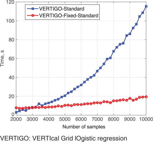
Time comparison of VERTIGO–Fixed-Standard and VERTIGO-Standard.
We tested the performance of our model with different number of parties k with a fixed sample size and changing the covariate size. We generated a random data set with each party data of size 10 000 × 200. The average computing time for training a LR model is given in table 3. The computational burden of our model is mainly related to the number of samples m, while the primal optimization computational burden is due to n. When k = 50, m = 10 000, n = 10 000, the computing time for primal optimization is more than 6 minutes, which is much higher than the time required for our method. Therefore, our model is faster than the classical method if data dimensionality n is high.
Table 3:
Average computing time in seconds for training LR models (m = 10 000)a
| k | VERTIGO | Primal optimization | |||||
|---|---|---|---|---|---|---|---|
| Standard | Fixed Standard | Lapack | Fixed Lapack | GPU | Fixed GPU | ||
| 2 | 108.3 | 26.4 (130) | 64.8 | 21.2 (130) | 47.9 | 18.5 (130) | 5.77 |
| 4 | 109.7 | 33.1 (241) | 64.9 | 32.2 (241) | 48.3 | 28.9 (241) | 9.47 |
| 6 | 118.4 | 41.3 (340) | 70.6 | 37.2 (340) | 52.8 | 37.1 (340) | 20.6 |
| 8 | 129.9 | 48.3 (430) | 78.7 | 45.0 (430) | 57.8 | 44.3 (430) | 26.5 |
| 10 | 134.1 | 55.5 (524) | 79.0 | 52.9 (524) | 57.8 | 52.7 (524) | 31.0 |
| 50 | 218.7 | NA | 129.3 | NA | 97.8 | NA | 416.8 |
Abbreviations: VERTIGO, vertical grid logistic regression; GPU, graphics processing unit; NA, not available.
aThe bold values correspond to the best performance models in terms of average computing time.
Real data
Genome data
To simulate a 3-site scenario, we used the breast cancer data set GSE3494.24 A total of 251 patient profiles were retrieved. There were 10 phenotype features and 1 outcome variable indicating that a patient died or survived. We removed 15 patients who had an unknown survival status. For the remaining 236 patients, each had 22 283 gene expression features on platform GPL96 and 22 654 gene expression features on platform GPL97, from which the top 15 features were selected based on the ranking of their P values (t test), as suggested by Osl.25 From Party 1, the top 15 genotype features on GPL96 served as data . From Party 2, the top 15 genotype features on GPL97 served as data . From Party 3, the 10-dimensional phenotype features served as data . As mentioned before, the binary responses were accessible to all parties. Figure 7 shows the results of this 3-node experiment on both discrimination and calibration, which are the same as those obtained with the model that used centralized primal optimization. There is also no difference (precision ∼ ) in terms of estimated parameters after 12 iterations. For this experiment, we set λ = 2 for VERTIGO (including standard, Lapack, and GPU). The parameter λ affects the number of iterations and convergence for Fixed-Hessian methods (including fixed-standard, fixed-Lapack, and fixed-GPU); we set λ = 1000 for them. As shown in figure 7, the global AUC value for VERTIGO is 0.940 ± 0.013, which is no different from the results of ordinary LR models using all data. Additionally, the H-L C test P value for VERTIGO is .709. The time cost for VERTIGO is roughly 2 times higher than for primal optimization, as shown in table 4. The speed degradation is not very obvious because the sample size was small. However, this can become a major concern when we are dealing with a cohort of thousands of patients.
Figure 7:

Performance of VERTIGO on the genome data set. The error bar in the calibration plot corresponds to a 95% confidence interval for predictions in each decile.
Table 4:
Average computing time in seconds for training logistic regression models (k = 3)
| VERTIGO | Primal optimization | ||||||
|---|---|---|---|---|---|---|---|
| Standard | Fixed Standard | Lapack | Fixed Lapack | GPU | Fixed GPU | ||
| Time, s | 0.11 | 0.10 (31) | 0.09 | 0.10 (31) | 0.12 | 0.10 (31) | 0.06 |
Abbreviations: VERTIGO, vertical grid logistic regression; GPU, graphics processing unit.
The bold value corresponds to the best performance model in terms of average computing time.
Myocardial infarction data
We also tested our method on the myocardial infarction data26 that contained 1253 records with 1 binary outcome and 35 features. We split the data set into to simulate a 3-part scenario. The binary responses were accessible to all parties. For this experiment, we set λ = 2 for the Newton implementation (including standard, Lapack, and GPU). We set λ = 80 for Fixed-Hessian methods (including fixed-standard, fixed-Lapack, and fixed-GPU). The results are given in figure 8 and table 5. The global AUC value for VERTIGO was 0.856 ± 0.009 and the H-L C test P value was .067. Although the average computing time of VERTIGO-Standard is about 1.16 seconds, which is 3 times higher than for primal optimization, it is acceptable for practical use.
Figure 8:

Performance of VERTIGO on the myocardial infarction data set. The error bar in the calibration plot corresponds to a 95% confidence interval for predictions in each decile.
Table 5:
Average computing time for training LR models (k = 3)
| VERTIGO | Primal optimization | ||||||
|---|---|---|---|---|---|---|---|
| Standard | Fixed Standard | Lapack | Fixed Lapack | GPU | Fixed GPU | ||
| Time, s | 1.16 | 10.40 (1553) | 0.80 | 9.88 (1553) | 0.79 | 9.98 (1553) | 0.36 |
Abbreviations: VERTIGO, vertical grid logistic regression; GPU, graphics processing unit.
The bold value corresponds to the best performance model in terms of average computing time.
MIMIC II data
We also tested our method over Multiparameter Intelligent Monitoring in Intensive Care (MIMIC II) Databases,27 which contain comprehensive data on 32 535 patients and over 40 000 intensive care unit (ICU) stays. The MIMIC II data set was collected between 2001 and 2008 from a variety of ICUs (medical, surgical, coronary care, and neonatal) in a single tertiary teaching hospital. We selected 41 features from the MIMIC II clinical database that contains clinical data from bedside workstations as well as from hospital archives. Selected features were gender, age, CO2, arterial blood pressure, SpO2, SaO2, arterial pH, total respiratory rate, white blood cell count, heart rate, as well as some comorbidity scores such as scores for congestive heart failure, cardiac arrhythmias, valvular disease, AIDS, lymphoma, etc. There were 4855 patients with these 41 common features. We used deceased or alive in the hospital as the response Y. For this experiment, we set λ = 2 for the Newton implementation (including standard, Lapack, and GPU). We set λ = 1300 for Fixed-Hessian methods (including fixed-standard, fixed-Lapack, and fixed-GPU). The results are shown in figure 9 and table 6. We can see that the AUC of our model is 0.761 ± 0.007 and the H-L C test P value is .232. The computing time was acceptable.
Figure 9:

Performance of VERTIGO on the MIMIC II data set. The error bar in the calibration plot corresponds to a 95% confidence interval for predictions in each decile.
Table 6:
Average computing time for training a logistic regression model (k = 2)
| VERTIGO | Primal optimization | ||||||
|---|---|---|---|---|---|---|---|
| Standard | Fixed Standard | Lapack | Fixed Lapack | GPU | Fixed GPU | ||
| Time, s | 19.27 | 15.91 (443) | 12.09 | 14.81 (443) | 9.98 | 15.08 (443) | 1.16 |
Abbreviations: VERTIGO, vertical grid logistic regression; GPU, graphics processing unit.
The bold value corresponds to the best performance model in terms of average computing time.
DISCUSSION
Limitations
We presented a proof of concept that building multivariate LR models using VERTIGO is practical and results in the same parameters (ie, coefficients and the intercept) that would be obtained if the data were centralized. We demonstrated 2 alternative algorithms based on fixed and varying Hessian matrices. The Fixed-Hessian approach shows efficiency advantage when dealing with large data but requires more communications to converge. The varying Hessian approach involves heavier computation and is slower for large data sets but needs less communication during optimization. Like other LR implementations (GLORE or SMO), VERTIGO may fail to estimate parameters when the class distribution is highly imbalanced (eg, 98% positive vs 2% negative cases). We can protect the intermediary statistics using secure communication protocols like Secure Sockets Layer (SSL) with 256-bit encryption, but a rigorous security model (eg, without a trusted hub or in the presence of malicious parties) still remains to be worked out.
We used vertically distributed synthetic and real biomedical data sets for our experiments, but we have not yet implemented this algorithm in pSCANNER. Our experience has been that health systems leaders and claims data owners are extremely excited about the possibility of collaborating in effectiveness research if they do not have to transmit their patient-level data to another institution. The proposed model does not rely on centralized solutions and is good for handling vertically partitioned data with high dimensionality and a small sample size. However, there is a technical challenge in scaling up federated LR when the sample size is large. Because a parameter is needed for each record (dual optimization) instead of for each covariate or feature (primal optimization), our algorithm has to invert a large Hessian matrix (m × m) when the number of patients m is large. This is an expensive operation of time complexity O(m3) and requires a lot of memory. We are planning different approaches to speed up the computation, eg, using parallelization (map-reduce) or GPU units. There are tradeoffs in these options, eg, computation on GPUs is very fast, but it has a memory bottleneck of 6 GB. If the data sets are large, this might require a divide-and-conquer strategy, which can be slowed down by bulk loading from the main memory.
CONCLUSION
The vertical LR algorithm demonstrated its accuracy and usability through our derivation and experiments. This technique allows researchers to estimate parameters for a multivariate model using a vertically partitioned database without sharing patient-level information.
CONTRIBUTORS
YL and XJ share first authorship and contributed the majority of the writing and conducted major parts of the experiments. SW conducted some experiments and contributed to the methodology. HX provided helpful comments on both methods and presentation. LO-M provided the motivation for this work, detailed edits, and critical suggestions.
COMPETING INTERESTS
None.
FUNDING
This work was supported by National Human Genome Research Institute grants K99HG008175 and R01HG007078, National Library of Medicine grants R00LM011392 and R21LM012060, and National Heart, Lung, and Blood Institute grant U54HL108460.
SUPPLEMENTARY MATERIAL
Supplementary material is available online at http://jamia.oxfordjournals.org/.
REFERENCES
- 1.Ohno-Machado L, Agha Z, Bell DS, et al. pSCANNER: patient-centered Scalable National Network for Effectiveness Research. J Am Med Inform Assoc 2014;21(4):621–626. doi:10.1136/amiajnl-2014-002751. [DOI] [PMC free article] [PubMed] [Google Scholar]
- 2.Karr AF, Lin X, Sanil AP, et al. Secure regression on distributed databases. J Comput Graph Stat 2005;14:263–79. doi:10.1198/106186005X47714. [Google Scholar]
- 3.Fienberg S, Fulp W, Slavkovic A, et al. Secure log-linear and logistic regression analysis of distributed databases. In: PSD ‘06 Proceedings of the 2006 CENEX-SDC Project International Conference on Privacy in Statistical Databases. Berlin: Springer-Verlag; 2006:277–290. [Google Scholar]
- 4.Yu H, Jiang X, Vaidya J. Privacy-preserving SVM using nonlinear kernels on horizontally partitioned data. Adv Knowl Discov Data 2006;3918:647–56. [Google Scholar]
- 5.Ghosh J, Reiter JP, Karr AF. Secure computation with horizontally partitioned data using adaptive regression splines. Comput Stat Data Anal 2007;51(12):5813–5820. [Google Scholar]
- 6.Slavkovic AB, Nardi Y, Tibbits MM. “Secure” logistic regression of horizontally and vertically partitioned distributed databases. In: ICDMW ’07 Proceedings of the Seventh IEEE International Conference on Data Mining Workshops. Washington, DC: IEEE Computer Society; 2007:723–728. [Google Scholar]
- 7.Kantarcioglu M. A survey of privacy-preserving methods across horizontally partitioned data. In: Aggarwal CC, Yu PS, eds. Privacy-Preserving Data Mining. Vol 34 New York, NY: Springer US; 2008:313–335. [Google Scholar]
- 8.Wu Y, Jiang X, Kim J, et al. Grid Binary LOgistic REgression (GLORE): building shared models without sharing data. J Am Med Inform Assoc 2012;19(5):758–764. [DOI] [PMC free article] [PubMed] [Google Scholar]
- 9.Yi X, Zhang Y. Privacy-preserving naive Bayes classification on distributed data via semi-trusted mixers. Inf Syst 2009;34(3):371–380. [Google Scholar]
- 10.Sanil AP, Karr AF, Lin X, et al. Privacy preserving regression modelling via distributed computation. In: KDD ’04 Proceedings of the tenth ACM ACM SIGKDD International Conference on Knowledge Discovery and Data Mining. New York, NY: ACM; 2004:677 doi:10.1145/1014052.1014139. [Google Scholar]
- 11.Karr AF, Lin X, Sanil AP, et al. Privacy-preserving analysis of vertically partitioned data using secure matrix products. J Off Stat 2009;25(1):125–138. [Google Scholar]
- 12.Vaidya J, Kantarcioglu M, Clifton C. Privacy-preserving Naïve Bayes classification. VLDB J 2008;17(4):879–898. [Google Scholar]
- 13.Vaidya J. A survey of privacy-preserving methods across. Privacy-Preserving Data Min 2008;34:337–358. [Google Scholar]
- 14.Nardi Y, Fienberg SE, Hall RJ. Achieving both valid and secure logistic regression analysis on aggregated data from different private sources. J Priv Confidentiality 2012;4(1):9. [Google Scholar]
- 15.Yu H, Vaidya J, Jiang X. Privacy-preserving SVM classification on vertically partitioned data. In: PAKDD ‘06 Proceedings of the 10th Pacific-Asia conference on Advances in Knowledge Discovery and Data Mining. Berlin: Springer-Verlag; 2006:47–56. doi:10.1007/11731139_74. [Google Scholar]
- 16.Minka TP. A comparison of numerical optimizers for logistic regression [technical report]. http://research.microsoft.com/en-us/um/people/minka/papers/logreg/minka-logreg.pdf. Published 22 Oct 2003. Revised 26 Mar 2007. Accessed April 7, 2015. [Google Scholar]
- 17.CRAN - Package glmnet Website. http://cran.r-project.org/web/packages/glmnet/index.html. Accessed April 7, 2015. [Google Scholar]
- 18.Jaakkola TS, Haussler D. Probabilistic Kernel Regression Models. In: The Seventh International Workshop on Artificial Intelligence and Statistics. San Francisco, CA: Morgan Kaufmann Publishers, Inc; 1999. [Google Scholar]
- 19.Hanley A, Mcneil J. The meaning and use of the area under a receiver operating characteristic (ROC) curve. Radiol 1982;143:29–36. [DOI] [PubMed] [Google Scholar]
- 20.Hosmer DW, Hosmer T, Le Cessie S, et al. A comparison of goodness-of-fit tests for the Logistic Regression model. Stat Med 1997;16(9):965–980. [DOI] [PubMed] [Google Scholar]
- 21.Duda RO, Hart PE, Stork DG. Pattern Classification. New York: John Wiley & Sons, Inc; 2012. [Google Scholar]
- 22.LAPACK — Linear Algebra PACKage Website. http://www.netlib.org/lapack/#_software. Accessed January 30, 2015.
- 23.Keerthi SS, Duan KB, Shevade SK, et al. A fast dual algorithm for kernel logistic regression. Mach Learn. 2005;61(1–3):151–65. doi:10.1007/s10994-005-0768-5. [Google Scholar]
- 24.GEO Accession viewer. National Center for Biotechnology Information Website. http://www.ncbi.nlm.nih.gov/geo/query/acc.cgi?acc=GSE3494. Accessed January 30, 2015. [Google Scholar]
- 25.Osl M, Dreiseitl S, Kim J, et al. Effect of data combination on predictive modeling: a study using gene expression data. AMIA Annu Symp Proc 2010:567–571. [PMC free article] [PubMed] [Google Scholar]
- 26.Kennedy RL, Burton AM, Fraser HS, et al. Early diagnosis of acute myocardial infarction using clinical and electrocardiographic data at presentation: derivation and evaluation of logistic regression models. Eur Heart J 1996;17(8):1181–1191. [DOI] [PubMed] [Google Scholar]
- 27.Saeed M, Villarroel M, Reisner AT, et al. Multiparameter intelligent monitoring in intensive care II: a public-access intensive care unit database. Crit Care Med 2011;39(5):952–60. doi:10.1097/CCM.0b013e31820a92c6. [DOI] [PMC free article] [PubMed] [Google Scholar]
- 28.Rockafellar RT. Convex Analysis. Princeton, NJ: Princeton University Press; 1970. [Google Scholar]