Abstract
Data from diffusion magnetic resonance imaging (dMRI) can be used to reconstruct fiber tracts, for example, in muscle and white matter. Estimation of fiber orientations (FOs) is a crucial step in the reconstruction process and these estimates can be corrupted by noise. In this paper, a new method called Fiber Orientation Reconstruction using Neighborhood Information (FORNI) is described and shown to reduce the effects of noise and improve FO estimation performance by incorporating spatial consistency. FORNI uses a fixed tensor basis to model the diffusion weighted signals, which has the advantage of providing an explicit relationship between the basis vectors and the FOs. FO spatial coherence is encouraged using weighted ℓ1-norm regularization terms, which contain the interaction of directional information between neighbor voxels. Data fidelity is encouraged using a squared error between the observed and reconstructed diffusion weighted signals. After appropriate weighting of these competing objectives, the resulting objective function is minimized using a block coordinate descent algorithm, and a straightforward parallelization strategy is used to speed up processing. Experiments were performed on a digital crossing phantom, ex vivo tongue dMRI data, and in vivo brain dMRI data for both qualitative and quantitative evaluation. The results demonstrate that FORNI improves the quality of FO estimation over other state of the art algorithms.
Keywords: Diffusion MRI, fiber orientation estimation, neighborhood information
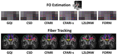
Graphical Abstract
1. Introduction
By capturing both the magnitude and the anisotropy of water diffusion, diffusion magnetic resonance imaging (dMRI) provides a noninvasive means to reconstruct fiber tracts, for example, in white matter and muscle (Johansen-Berg and Behrens, 2013). Diffusion tensor imaging (DTI), which is a basic dMRI strategy, models the water diffusion using a symmetric positive definite tensor (Basser et al., 1994). Since DTI is known to be insufficient to represent crossing fiber tracts, more advanced dMRI techniques, such as high angular resolution diffusion imaging (HARDI) (Tuch et al., 2002) and diffusion spectrum imaging (DSI) (Wedeen et al., 2005), have been developed.
In order to carry out tractography (Mori et al., 1999; Basser et al., 2000; Qazi et al., 2009; Reisert et al., 2011) and volumetric fiber tract segmentation (Bazin et al., 2011; Nazem-Zadeh et al., 2011; Yendiki et al., 2011; Ye et al., 2015b), fiber orientations (FOs) are computed from the dMRI data. In tractography, fiber streamlines are propagated according to the computed FOs or the distribution of FOs, and in volumetric tract segmentation the FO is a key feature upon which the voxels are labeled. Since accurate estimation of FOs is critical in these algorithms, it has been a major topic of research. For example, spherical deconvolution (Tournier et al., 2004, 2007; Cheng et al., 2014; Jeurissen et al., 2014), q-ball reconstruction (Tuch, 2004; Hess et al., 2006; Descoteaux et al., 2007), multi-tensor models (Landman et al., 2012; Peled et al., 2006; Behrens et al., 2007; Ramirez-Manzanares et al., 2007; Zhou et al., 2014; Liu et al., 2015; Ye et al., 2014), and ensemble average propagator methods (Michailovich et al., 2011; Rathi et al., 2014; Wedeen et al., 2008; Pickalov and Basser, 2006; Özarslan et al., 2006; Merlet and Deriche, 2013) have been developed so that multiple FOs can be estimated in each voxel.
A large number of diffusion gradient directions may be required to accurately estimate FOs when fiber tracts cross, which takes a long acquisition time and limits the use of dMRI in clinical practice (Bilgic et al., 2012). Therefore, methods have been developed to reduce the required number of gradient directions so that the dMRI acquisition is clinically achievable. Because the number of crossing FOs in a voxel is small, modeling the diffusion data as having arisen from a sparse subset of basis sources and solving the resulting optimization problem using sparsity regularization is particularly effective (Ramirez-Manzanares et al., 2007; Landman et al., 2012; Daducci et al., 2014; Merlet et al., 2012; Zhou et al., 2014; Michailovich et al., 2011; Rathi et al., 2014). The basis has been selected to be prolate diffusion tensors (Ramirez-Manzanares et al., 2007; Landman et al., 2012; Daducci et al., 2014; Zhou et al., 2014), spherical ridgelets (Michailovich et al., 2011; Rathi et al., 2014), and spherical polar Fourier basis (Merlet et al., 2012).
Noise can have a deleterious effect on FO estimation, especially in areas where fibers cross (Cheng et al., 2006; Aranda et al., 2014). A 3D toy example of two crossing tracts is shown in the axial view (the x–y plane) in Figure 1(a), where noise is added to the simulated dMRI data. Here, the CFARI algorithm (Landman et al., 2012) estimates FOs at each voxel independently; it yields noisy estimates and occasionally fails to yield a second direction at all (Figure 1(a)).
Figure 1.
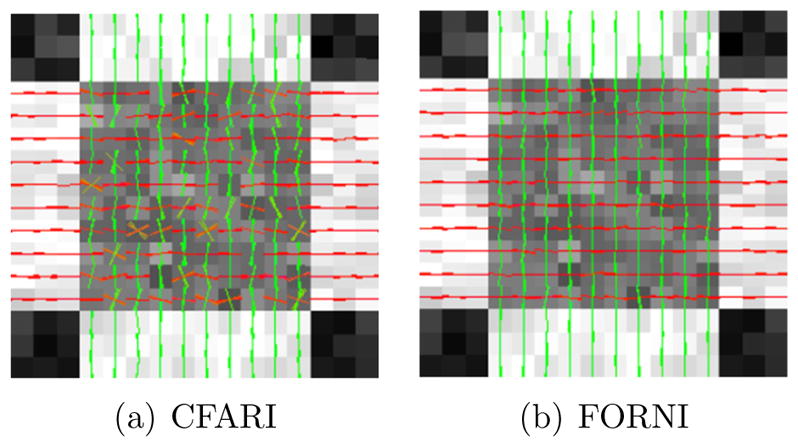
A 3D toy example of FO estimation on two simulated crossing tracts in the axial view (the x–y plane): (a) voxelwise FO estimation using the CFARI algorithm (Landman et al., 2012) and (b) FOs estimated by the proposed method (FORNI) incorporating spatial coherence of FOs.
To reduce the effect of noise, spatial coherence (or smoothness) has been used to improve FO estimation. In Becker et al. (2014) diffusion weighted images are smoothed before FO estimation. In Sigurdsson and Prince (2014), FOs are smoothed after voxelwise estimation using the CFARI method. In Duits and Franken (2011), FOs are smoothed using left-invariant diffusions on the space of positions and orientations. Tournier et al. (2013) and Reisert and Kiselev (2011) incorporate the continuity of FOs as regularization terms in the estimation to enforce FO smoothness, but sparsity regularization is not used. There are also methods that seek to simultaneously estimate and smooth FOs by combining spatial continuity with sparsity. In Michailovich et al. (2011) and Rathi et al. (2014), the TV-norm of diffusion weighted images is incorporated as a smoothness regularization term in the objective function. In Ramirez-Manzanares et al. (2007) and Zhou et al. (2014), spatial consistency of FOs is encouraged by adding regularization terms that smooth the mixture fractions of each basis tensor. However, spatial coherence is preserved in an indirect way in Michailovich et al. (2011), Rathi et al. (2014), Ramirez-Manzanares et al. (2007), and Zhou et al. (2014) because the objective functions do not explicitly model and smooth the directional information in the FOs. Recently, Auría et al. (2015a) define a spatially structured sparsity regularization term to incorporate directional information in the sparse reconstruction of FOs.
In this paper, we present the method Fiber Orientation Reconstruction using Neighborhood Information (FORNI), which is an FO estimation algorithm that incorporates spatial coherence. Preliminary results of this work were presented in a conference paper (Ye et al., 2016). An example of the FORNI FO estimation on the toy example in Figure 1(a) is shown in Figure 1(b). In contrast to most previous works, we form an objective function that directly encodes the directional information in the neighborhood to encourage spatial coherence of FOs. Specifically, a fixed tensor basis is used to represent diffusion weighted signals, which has the advantage of providing an explicit relationship between the basis and FOs. Spatial coherence is encouraged using weighted ℓ1-norm regularization, where the interaction of directional information in neighboring voxels is modeled. In the weighted ℓ1-norm regularization terms, basis directions that are more consistent with the FOs in the neighborhood are encouraged. Data fidelity is encouraged using a term that measures agreement between the observed and reconstructed diffusion signals. The resulting objective function is minimized using a block coordinate descent algorithm, and a straightforward parallelization strategy is used to speed up processing.
The remainder of the paper is organized as follows. Section 2 describes the FORNI algorithm and Section 3 presents the experiments on a digital crossing phantom, ex vivo tongue dMRI data, and in vivo brain dMRI data for qualitative and quantitative evaluation. Section 4 discusses the results and future works. Finally, Section 5 concludes the paper.
2. Methods
In this section, we first provide a background on diffusion signal modeling using a fixed tensor basis. Then, we describe our approach to the incorporation of directional information from neighboring voxels to improve FO estimation. Finally, the resulting objective function and the optimization strategy are presented.
2.1. A Multi-tensor Model with a Fixed Tensor Basis
Using the unified framework presented in Jian and Vemuri (2007), the diffusion weighted signal at each voxel can be modeled as
| (1) |
where x is a point on a smooth manifold ℳ, S(q) is the diffusion weighted signal with the diffusion gradient q, S0 is the baseline signal without diffusion weighting, f(x) is a probability density function, and R(q, x) is a kernel function.
The diffusion signals can be represented by a basis, and one commonly used basis is a set of fixed prolate tensors (Landman et al., 2012; Zhou et al., 2014; Ramirez-Manzanares et al., 2007; Daducci et al., 2014). The primary eigenvector (PEV) of each basis tensor represents a possible FO and is referred to as a basis direction. In this work, we use the tensor basis comprising N = 289 prolate tensors Di whose PEVs vi are approximately evenly oriented over the unit sphere. These basis directions were determined by tessellating an octahedron, and the number of basis directions (N = 289) lies in the range of previously used numbers (Ramirez-Manzanares et al., 2007; Landman et al., 2012; Auría et al., 2015a). The shape of the basis tensor is determined by its eigenvalues (λ1 ≥ λ2 ≥ λ3 > 0). The second and third eigenvalues are set equal, and each eigenvalue is determined by examining the diffusion tensors of a noncrossing fiber tract (Landman et al., 2012).
With this tensor basis, we have ℳ = 𝒮2 (a unit sphere), x = v (a unit vector), f(v) = fiδ(v; vi), and R(q, vi) = e−qTDiq (based on the Stejskal-Tanner tensor formulation (Stejskal and Tanner, 1965)). By normalizing the diffusion gradient as q̃ = q/|q|, the gradient direction q̃ is associated with a constant b determined by the imaging sequence. Taking image noise into account, Eq. (1) then becomes (Landman et al., 2012)
| (2) |
where fi is the (unknown) nonnegative mixture fraction for Di, , and n(q) is noise.
After defining y(q) = S(q)/S0 and η(q) = n(q)/S0 and letting K be the number of diffusion gradient measurements, Eq. (2) can be written as
| (3) |
where y = (y(q1), y(q2), …, y(qK))T, G is a K×N matrix comprising the attenuation terms , f = (f1, f2, …, fN)T, and η = (η(q1), η(q2), …, η(qK))T. Because the number of FOs at each voxel is usually small with respect to the number of diffusion gradients, the mixture fractions can be estimated using the following sparse reconstruction formulation
| (4) |
To solve Eq. (4), the constraint of is relaxed (Landman et al., 2012; Ramirez-Manzanares et al., 2007) and then the ℓ0-norm is replaced by the ℓ1-norm, yielding the following simpler problem,
| (5) |
After solving this, the estimated vector f̂ is normalized so that its elements add to one. Note that in this paper we interpret small mixture fractions as components of isotropic diffusion; therefore, FOs are given by those basis directions whose mixture fractions are greater than a threshold fth. Accordingly, by focusing on the estimation of mixture fractions, we are also estimating the FOs.
2.2. FO Estimation Using Neighborhood Information
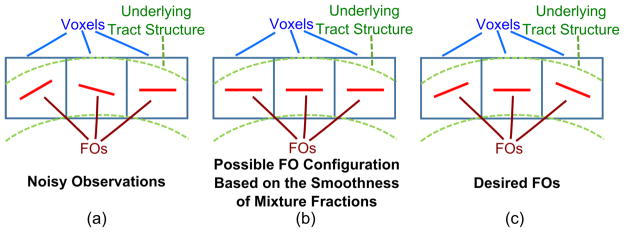
Incorporation of spatial coherence in the estimation of FOs can reduce the effects of noise (Michailovich et al., 2011). Some researchers have incorporated neighborhood information in order to maintain smoothness of mixture fractions (Ramirez-Manzanares et al., 2007; Zhou et al., 2014). But having smooth mixture fractions does not equate to having smooth FO angles. For example, suppose we have three side-by-side voxels a, b, and c, whose mixture fractions are fa = (1, 0, …, 0)T, fb = (0, 1, 0, …, 0)T, and fc = (0, 0, 1, 0, …, 0)T, respectively. The magnitude of the difference ||fa − fb|| between the mixture fractions of a and b is the same as the magnitude of the difference ||fa − fc|| between a and c, while the desired measure of difference should be related to the angles between the basis directions with nonzero mixture fraction entries. Figure 2 gives a graphical example of a curved tract, where simply using the smoothness of mixture fractions could lead to identical FOs along the tract instead of a desired gradually-changing FO structure. This limitation exists in the case of crossing fibers as well. In this work, we encourage spatial coherence of FOs by explicitly incorporating the directional information in neighboring voxels into the FO estimation. The symbols used in FORNI are listed in Table 1.
Figure 2.
A graphical example showing the potential difficulties when the smoothness of mixture fractions is used to represent spatial coherence of FOs.
Table 1.
Symbols used in FORNI
| Symbol | Definition |
|---|---|
| vi | Basis direction |
| i, q | Index for basis directions |
| N | Number of basis directions |
| G | Dictionary matrix containing attenuation terms |
| m, n, m0, m1 | Index for voxels |
| M | Number of voxels |
| wm,n | Voxel similarity between m and n |
| 𝒩m | Neighborhood of m |
| Dm | Diffusion tensor at m |
| ym | Diffusion signal at m |
| fm | Mixture fraction at m |
| f̂m | Estimated mixture fraction at m |
| f̃m | Normalized mixture fraction estimate at m |
| fm,i | Entry of fm |
| fth | Mixture fraction threshold |
| wm,j | FO at m |
| j | Index for FOs |
| 𝒲m | The set of all FOs at m |
| um,p | Likely FO at m |
| p | Index for likely FOs |
| 𝒰m | The set of all likely FOs at m |
| Cm | Weighting matrix at m |
| Cm,i | Diagonal entry of Cm |
| α, β, μ | Parameters in FORNI |
| rm,n(i) | Basis-neighbor similarity |
| Rm(i) | Aggregate basis-neighbor similarity |
| θR | An angle threshold |
| t | Index for iterations |
| Np | Number of voxels processed in parallel |
2.2.1. FO Estimation with Known Neighborhood Information
First, we consider a simplified case where the mixture fractions fm are to be estimated in the voxel m and the mixture fractions are known at all voxels in a neighborhood 𝒩m of voxel m. Let n be a voxel in 𝒩m and let voxel n have mixture fractions fn; then the FOs at voxel n are given by the set
| (6) |
where fn,i is the i-th element of fn, and fth is the threshold for mixture fractions. We further let , where wn,j is the j-th FO in voxel n and Wn is the cardinality of 𝒲n. For concreteness, we assume at this stage and for the remainder of the paper that the neighborhood consists of the nearest 26 neighbors (Auría et al., 2015a) and fth = 0.1 (Landman et al., 2012). We want to estimate the mixture fractions fm (and therefore the associated FOs using Eq. (6)) at voxel m given the neighborhood information.
Our main goal is to use the patterns of FOs in the neighboring voxels to encourage a similar pattern of FOs in voxel m—this is the idea of FO smoothness or coherence. A set 𝒰m of likely FOs for the voxel m can be computed given knowledge of the mixture fractions and FOs in its neighbors (the details will be described later). The likely FO information is then used to influence the mixture fraction estimation in voxel m using the sparse estimation framework previously described (for the incorporation of prior knowledge in FO estimation) in the FIEBR algorithm (Ye et al., 2015a). In particular, we solve the following weighted ℓ1-norm regularized least squares problem
| (7) |
where Cm is a diagonal matrix that weights the basis directions according to their distance to the likely FOs in 𝒰m. For example, the basis directions vi that are closer to the likely FOs in 𝒰m have smaller weights in the weighted ℓ1-norm; therefore, they have smaller penalty in the objective function and are more likely to be selected as FOs in m.
Ye et al. (2015a) specified the diagonal entries of Cm as
| (8) |
where um,p ∈ 𝒰m, Um is the cardinality of 𝒰m, and α ∈ [0, 1) is a constant. Since vi and um,p are unit vectors, |vi · um,p| ∈ [0, 1] and Cm,i is positive for all i. In this work, we find it useful to normalize these diagonal entries so that the weights on the most likely FOs are nearly the same as when there is no neighboring FO information used at all. Accordingly, here we specify the diagonal weights in Cm as
| (9) |
We see that the weights in Eq. (9) are just the weights in Eq. (8) normalized by the smallest diagonal entry. Note that we require α ∈ [0, 1) in order to ensure that Cm,i > 0, ∀i.
Ye et al. (2015a) developed the above framework to incorporate fixed prior directions at each voxel in the estimation of FOs. These prior directions were either hand-drawn or determined by atlas registration. To apply this framework to spatial smoothness, we replace the concept of prior directions with that of likely FOs. Note that our application of FO estimation with spatial coherence is fundamentally different than Ye et al. (2015a) in two respects: 1) likely FOs are computed based on neighbors and no manual intervention or anatomical atlas registration is needed; 2) because computations of FOs depend on neighbors, the FOs for all voxels need to be simultaneously estimated and the independent FO computation at each voxel in Eq. (7) is inappropriate. The proposed approach to the computation of likely FOs and simultaneous FO estimation is presented next in Sections 2.2.2 and 2.2.3, respectively.
2.2.2. Computation of Likely FOs from Neighbors
A flow chart of the likely FO computation at each voxel is shown in Figure 3. We first consider a single neighbor voxel; in particular, let voxel n be the neighbor of voxel m. Let Dm and Dn be the diffusion tensors fit from diffusion weighted signals at voxels m and n, respectively. Based on the tensors, we define the voxel similarity wm,n between voxels m and n as
Figure 3.
A flow chart of the likely FO computation at a voxel.
| (10) |
where μ is a constant and d(·, ·) is the measure of distance between tensors given by Arsigny et al. (2006)
| (11) |
Given the definition of voxel similarity, we now want a measure of the similarity of each basis direction vi to the FOs in voxel n. Accordingly, we define the basis-neighbor similarity rm,n(i) as
| (12) |
In order for a given basis vector to be similar to a neighbor’s computed FO, the voxels must be similar and the directions must be well-aligned.
Now consider all voxels that are neighbors of voxel m. We define an aggregate basis-neighbor similarity Rm(i) at voxel m for each basis vector vi as
| (13) |
Basis directions with larger aggregate basis-neighbor similarity correspond to directions that are close to FOs in many neighboring voxels or in a few neighbors that have strong voxel similarity. These are directions that are more likely to be FOs in voxel m by virtue of the current FOs in neighboring voxels.
Given Rm we can extract a set of likely FOs for voxel m. We could simply choose the directions with the largest Rm values or those with Rm values greater than a threshold. However, a special circumstance should be noted. In a crossing region, such as that depicted in Figure 4(a), some of the neighboring voxels could fail to estimate a crossing FO due to noise. In particular, suppose there are two crossing FOs ṽ1 and ṽ2 in this region, and ṽ1 fails to be reconstructed in more than one neighboring voxel while the other neighbors have both FOs reconstructed. In this case, as is shown in Figure 4(b), the basis vector vi corresponding to ṽ1 could have a smaller Rm(i) value than a basis direction ṽ3, for example, which is distant from both ṽ1 and ṽ2. In this case, the desired ṽ1 is not included in the top two likely FOs and thus ṽ1 may not be properly encouraged, while an undesired ṽ3 may be encouraged and create false FOs.
Figure 4.
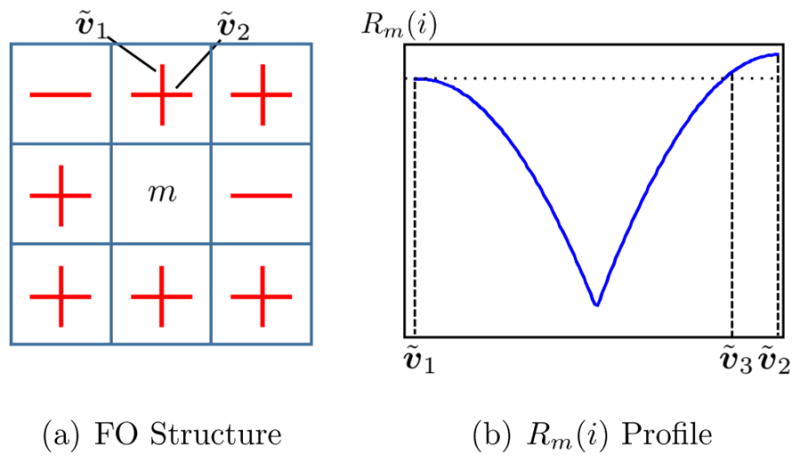
An illustration of the Rm(i) profile in the case where one of the crossing FOs fails to be reconstructed in some neighboring voxels.
A more robust definition of the likely FOs is as those directions which comprise the local maxima of Rm. In particular, consider the direction vi and compare its value Rm(i) to all values of Rm(i′) corresponding to directions vi′ within θR = 20°. If Rm(i) is maximum, then vi is included in the likely FOs. Following this reasoning, the likely FOs at voxel m are given by
| (14) |
Note that θR is converted to have a unit of radians so that it can be compared with arccos(|vi · vi′ |).
An example of the Rm values of a voxel in the crossing region in Figure 1 is shown in Figure 5, where the Rm values are plotted on the unit sphere according to their associated basis directions. The Rm values of the likely FOs are indicated by the larger dots and black arrows. The two likely FOs are the horizontal (x) and vertical (y) directions in Figure 1 that correspond to the desired FOs.
Figure 5.
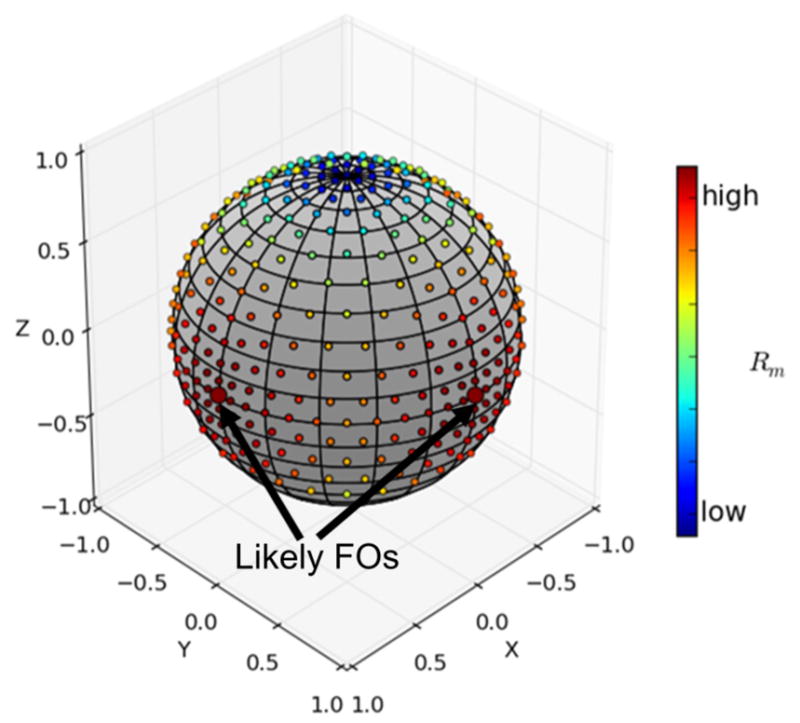
An example of the Rm values of a voxel in the crossing region in Figure 1. Each Rm(i) is plotted on the unit sphere according to its associated basis direction vi. The Rm values of the likely FOs are indicated by the larger dots and black arrows.
2.2.3. FO Estimation for All Voxels
After the likely FOs for voxel m are determined, the weighting matrix Cm can be obtained. Note that in Eq. (7), we have assumed known neighbor information. However, the FOs in the neighboring voxels are also unknown and must be estimated, which means that FOs cannot be estimated independently—it is a joint FO estimation problem.
Suppose the total number of voxels of interest is M. The estimation of all unknown mixture fractions (through which the FOs are also estimated) can be written as
| (15) |
Here Cm encodes the interaction between neighbors. Since Cm depends on the parameter α (see Eq. (9)), α and β are the two parameters that must be specified by the user. When α is larger there is more influence from neighboring voxels, and when β is larger the mixture fractions tend to be more sparse and therefore there are fewer estimated FOs.
2.3. Minimization of the Objective Function and Parallelization
In Eq. (15), the FOs in each voxel are coupled with neighbor voxels in the weighting matrix Cm. We use an iterative block coordinate descent (BCD) method (Bertsekas, 1999) to decouple the interaction and optimize the objective function. At iteration t, each fm is estimated by solving
| (16) |
| (17) |
where is the diagonal weighting matrix at iteration t and it is determined by the likely FOs computed from the neighbor FOs at iteration t or t − 1 according to Eq. (9). The detailed update of at each iteration and the optimization of Eq. (17) are given in Appendix A. Finally, is normalized so that entries sum to unity and the FOs at voxel m at time t are determined using Eq. (6).
Because the ℓ1-norm regularized least squares problem in Eq. (17) must be solved for every voxel in each iteration, the algorithm requires heavy computation and can be time-consuming. Therefore, we modified the BCD optimization in Eq. (17) so that multiple voxels can be simultaneously solved to speed up processing. We process Np ≥ 2 voxels together (in this work Np = 8). Each voxel m can be represented as m = aNp + b, where a and b are integers ( and 1 ≤ b ≤ Np). For each group aNp + 1 ≤ m ≤ (a + 1)Np with fixed a, we have
| (18) |
and these fm’s can be solved in parallel.
The above iterative algorithm is initialized using CFARI (Landman et al., 2012), which provides the mixture fractions at each voxel independently. The algorithm terminates when the FO difference between two successive iterations is small or when the maximum number of iterations is reached. The complete algorithm is summarized in Algorithm 1.
Algorithm 1.
FORNI
| Input: Diffusion weighted signals ; baseline signals without diffusion weighting; diffusion gradients {q1, …, qK}; size of parallel processing: Np; the tensor basis and their PEVs ; maximum number of iterations tmax; the initialization of FOs computed from Landman et al. (2012); the iteration number starts from t = 1; | |
| Output: Mixture fractions and FOs | |
| 1: | Compute the attenuation matrix G: |
| 2: | Compute : ym = (Sm(q1)/S0m, …, Sm(qK)/S0m)T |
| 3: | Initialize FOs: |
| 4: | while t ≤ tmax do |
| 5: | for do |
| 6: | parfor b = 1 : min(Np, M − aNp) do |
| 7: | m := aNp + b |
| 8: | for all basis directions vi do |
| 9: | |
| 10: | end for |
| 11: | |
| 12: | for i = 1 : N do |
| 13: | |
| 14: | end for |
| 15: | Solve Eq. (17) to obtain |
| 16: | |
| 17: | end parfor |
| 18: | for b = 1 : min(Np, M − aNp) do |
| 19: | m := aNp + b |
| 20: | 𝒲m := {vi|fm,i > fth, i = 1, …, N} |
| 21: | end for |
| 22: | end for |
| 23: | t := t + 1 until convergence |
| 24: | end while |
| 25: | return nd |
3. Experiments
FORNI was evaluated first on a digital crossing phantom, then on ex vivo tongue dMRI data from one subject, and finally on an in vivo brain dMRI dataset comprising six subjects. FORNI was compared to the SHORE algorithm (Merlet and Deriche, 2013) which estimates the ensemble average propagator and orientation distribution function using the SHORE basis (Cheng et al., 2011), the constrained spherical deconvolution (CSD) algorithm (Tournier et al., 2007) which introduces a nonnegative constraint on the spherical harmonics framework, the CFARI algorithm that estimates the FOs using a voxelwise sparse reconstruction (Landman et al., 2012), an FO smoothing algorithm (CFARI-s) (Sigurdsson and Prince, 2014) that smooths the CFARI results, and an FO estimation algorithm (L2L0NW) (Auría et al., 2015a) that uses structured sparsity to enforce smooth FO estimation. In the experiments on the tongue dMRI data, we have also compared our method with the FIEBR algorithm (Ye et al., 2015a) that is designed for the tongue to improve FO estimation by using atlas information. In the experiments on brain dMRI, because multiple b-values were used to acquire the brain dMRI data, the CSD algorithm was replaced by generalized q-sampling imaging (GQI) (Yeh et al., 2010) which can reconstruct FOs using multishell dMRI. SHORE and CSD are implemented using the Dipy software (Garyfallidis et al., 2014) (http://nipy.org/dipy/documentation.html); CFARI and CFARI-s are implemented in the JIST software framework (Lucas et al., 2010); GQI is implemented in the DSI Studio software (http://dsistudio.labsolver.org/Manual/Reconstruction); and L2L0NW was performed using the code provided by its authors at https://github.com/basp-group/co-dmri.
3.1. 3D Digital Crossing Phantom
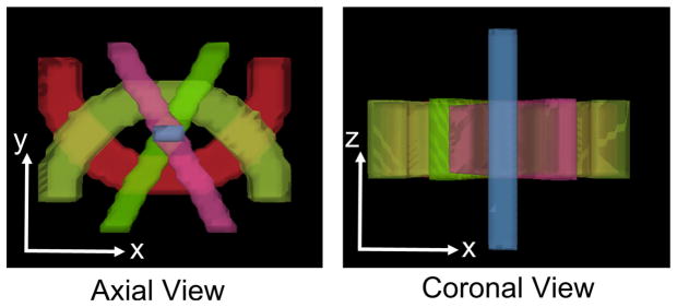
A 3D digital crossing phantom (available at https://www.iacl.ece.jhu.edu/Chuyang) was generated to simulate five fiber tracts (see Figure 6), where one b0 image and 60 gradient directions (b = 1000 s/mm2) were used. A two-tensor/three-tensor model was used to create the simulated diffusion signals for regions with two/three crossing tracts. The eigenvalues of each individual tensor are λ1 = 2.0 × 10⁻³ mm2/s and λ2 = λ3 = 0.5 × 10⁻³ mm2/s. Thus, for each individual tensor the fractional anisotropy (FA) is 0.71 and the mean diffusivity (MD) is 1.0×10⁻³ mm2/s. Rician noise with different signal-to-noise ratio (SNR) (SNR = 10, 20, and 30) on the b0 image was added to the diffusion weighted images (DWIs).
Figure 6.
A 3D rendering of the simulated tracts.
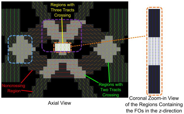
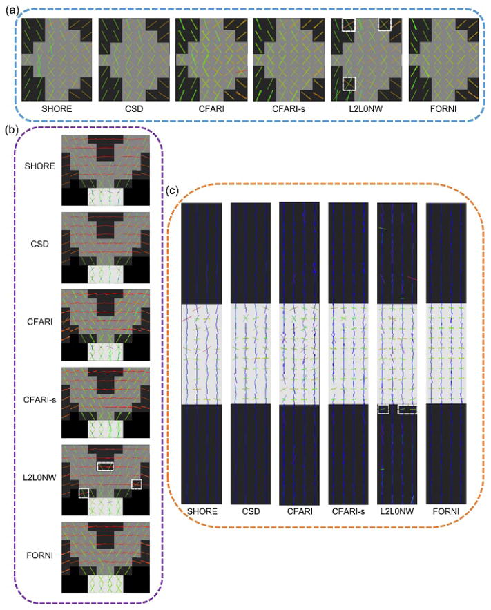
FORNI (with α = 0.8, β = 0.5, and μ = 3.0) was applied and compared with SHORE (Merlet and Deriche, 2013), CSD (Tournier et al., 2007), CFARI (Landman et al., 2012), CFARI-s (Sigurdsson and Prince, 2014), L2L0NW (Auría et al., 2015a), and the ground truth. The ground truth FOs are shown in Figure 7. Because the FOs in the z-direction are not visible in the axial view, the regions containing these FOs are also shown in the coronal view. A qualitative evaluation of FO estimation is shown in Figure 8 using the results at SNR = 20 in the highlighted regions in Figure 7. The FOs are color-coded by the standard DTI color scheme (red: left–right; green: front–back; and blue: up–down) (Pajevic and Pierpaoli, 1999) and overlaid on the map indicating the number of ground truth FOs at each voxel. We can see that FORNI produces smooth FOs compared with SHORE, CSD, and CFARI which perform voxelwise FO estimation. In the regions (highlighted by the orange box in Figures 7 and 8) containing three crossing tracts, both L2L0NW and FORNI are able to better recover the crossing patterns than SHORE, CSD, CFARI, and CFARI-s. In addition, FORNI does not produce false positive FOs (see the white boxes in Figure 8) as in the results of L2L0NW when neighbor information is used.
Figure 7.
Ground truth FOs overlaid on the map indicating the number of FOs at each voxel. The FOs in the z-direction are shown in a coronal view. The regions highlighted by the dashed boxes are later zoomed in for qualitative evaluation in Figure 8. The visualization of FOs was created in FSLView (Jenkinson et al., 2012).
Figure 8.
FO estimation results overlaid on the map indicating the number of ground truth FOs at each voxel at SNR = 20 in the regions highlighted in Figure 7. Note the white boxes where L2L0NW produces false positive FOs. The visualization of FOs was created in FSLView (Jenkinson et al., 2012).
To quantitatively evaluate the results, we define a voxelwise error measure of FOs in degrees:
| (19) |
Here, wi and uj are the estimated and ground truth FOs, respectively, and N1 and N2 are the numbers of wi and uj, respectively. Note that arccos(·) is in radians and it is converted to degrees by multiplying . In the max function of Eq. (19), the first term measures how far away the estimated FOs are from the true FOs, and the second term measures how accurate the true FOs are estimated. Since both terms are expected to be small when the FO estimation is accurate, the worst of the two errors is reported.
We compared the FO errors of FORNI over the entire phantom with those of SHORE, CSD, CFARI, CFARI-s, and L2L0NW using all three noise levels. The results are shown in Figure 9, where means and standard deviations of the FO errors are plotted. It can be seen for all methods the FO errors increase as SNR decreases. FORNI produces more accurate FOs than the competing methods in all three cases.
Figure 9.
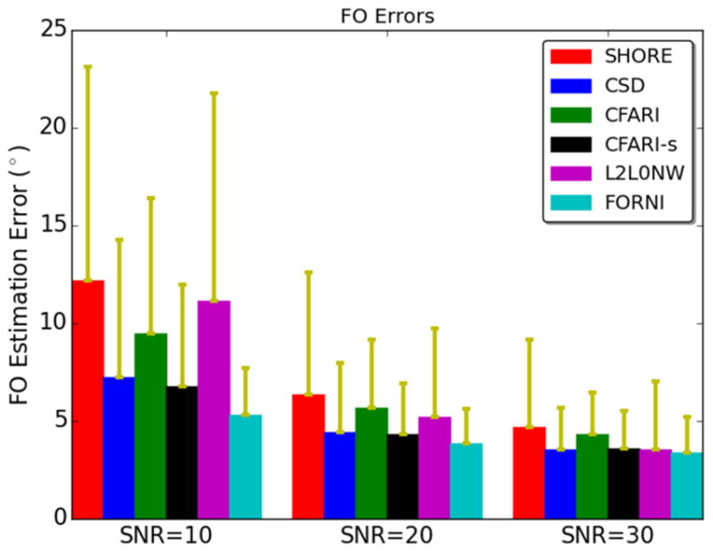
Means and standard deviations of FO errors over the entire phantom at SNR = 10, 20, and 30.
Next, we studied the effect of the parameters, mixture fraction thresholds, and initialization in FORNI. Because in the tongue and brain dMRI data used in this work, the SNR is close to 20 on the b0 images, we used the phantom at SNR = 20 for the evaluation below.
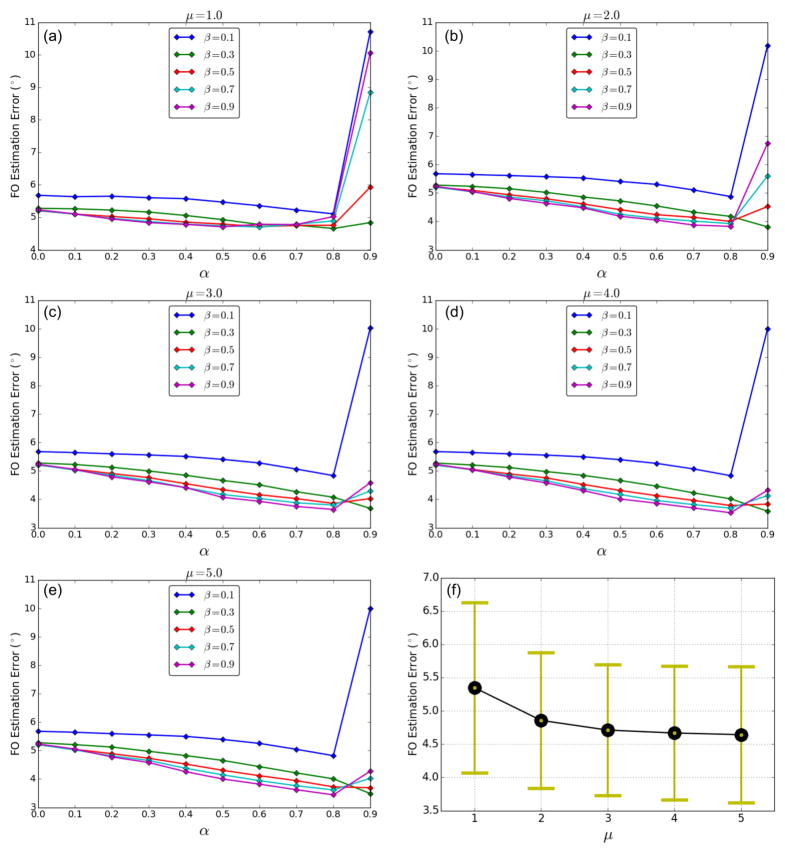
To evaluate the impact of parameters, we experimented with different α, β, and μ settings: α ∈ {0.0, 0.1, …, 0.9}, β ∈ {0.1, 0.3, …, 0.9}, and μ ∈ {1.0, 2.0, …, 5.0}. The average FO errors for each α, β, and μ combination over the entire phantom are plotted in Figures 10(a)–(e). Note that when α = 0.0, the basis directions are uniformly weighted and no neighbor information is used, which is equivalent to the CFARI algorithm. At each μ for most β, increasing α reduces FO errors until α is too large, and in most cases incorporation of neighborhood information (α > 0) improves the estimation accuracy. Figure 10(f) gives the means and standard deviations of these average FO errors using all α and β combinations at each μ. It can be seen that the error starts to become stable when μ reaches 3.0. In addition, the variance is smallest at μ = 3.0, indicating the performance is less affected by changing α and β values than at other μ. Therefore, for our real data application, we use μ = 3.0. Then, at μ = 3.0 we select α and β for the real data experiments with the following rationale. First, because in many cases α = 0.9 causes errors even larger than those without neighbor information, we only consider the choices with α < 0.9. Second, we have found from experience that choosing β too large can lead to instabilities in the ℓ1 solver. Therefore, we have picked α = 0.8 and β = 0.5 for the remaining experiments. From Figure 10(c), we see that at μ = 3.0 this selection yields a performance that is comparable to the other four top performing operating points.
Figure 10.
Average FORNI FO errors over the entire phantom at SNR = 20 with different α, β, and μ: (a)–(e) μ = 1.0, 2.0, …, 5.0; (f) means and standard deviations of the data points in (a)–(e) at different μ.
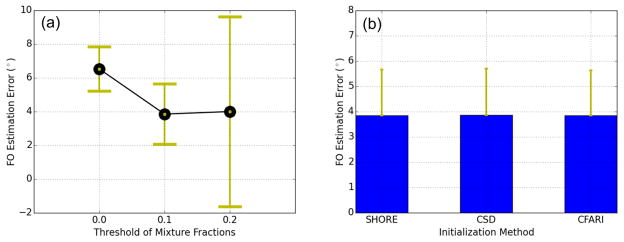
Using the selected (α, β, μ) = (0.8, 0.5, 3.0), we computed the FO errors with different mixture fraction thresholds (fth ∈ {0.0, 0.1, 0.2}) and different initialization methods including SHORE, CSD, and CFARI, which are the voxelwise FO estimation algorithms evaluated in this work. The results are shown in Figure 11. In Figure 11(a), we can see that fth = 0.1 (as selected in Section 2.2.1) achieves the smallest error. In Figure 11(b), different initialization methods achieve very close FO errors in FORNI, which indicates the robustness of FORNI to initialization.
Figure 11.
Means and standard deviations of FORNI FO errors at SNR = 20 with different (a) mixture fraction thresholds and (b) initialization methods.
3.2. Ex Vivo Tongue dMRI
Next, FORNI (with α = 0.8, β = 0.5 and β = 3.0) was applied to the ex vivo tongue dMRI data. Nine b0 images and 64 DWIs (b = 2000 s/mm2) were acquired on a 3T MRI scanner (Magnetom Trio, Siemens, Erlangen, Germany). The resolution is 2 mm isotropic (matrix size: 100 × 100) and the number of slices is 30. The SNR on the b0 image is approximately 20.31, which was estimated by placing bounding boxes in the background and tract regions (Ye et al., 2015a). Eddy current correction and diffusion tensor estimation were performed by CATNAP (Landman et al., 2007) implemented in the JIST software (Lucas et al., 2010). According to the tensors in noncrossing regions, the eigenvalues of the basis tensors used in FORNI were λ1 = 7.0×10⁻⁴ mm2/s and λ2 = λ3 = 3.0×10⁻⁴ mm2/s. The FORNI processing took around seven minutes for the data. SHORE (Merlet and Deriche, 2013), CSD (Tournier et al., 2007), CFARI (Landman et al., 2012), CFARI-s (Sigurdsson and Prince, 2014), L2L0NW (Auría et al., 2015a), and FIEBR (Ye et al., 2015a) were also applied on the data.
Figure 12 shows results in the coronal view with the focus on the crossing region of the genioglossus (GG) and the transverse (T) muscle in the tongue. A high resolution structural image with a schematic of the anatomy of GG and T is shown in Figure 12(a) for location reference. It can be seen that FORNI not only produces smoother FOs but also better reconstructs the crossing FOs of GG and T.
Figure 12.
FO estimation on the ex vivo tongue in the coronal view, which is focused on the crossing (highlighted by the white dashed box in (a)) of the GG and T muscle. A high resolution structural image (left) with a schematic of the anatomy of GG and T is shown for location reference.
3.3. In Vivo Brain dMRI
FORNI was applied to the six subjects in an in vivo brain dMRI dataset. The images were acquired on a 3T MRI scanner (Magnetom Trio, Siemens, Erlangen, Germany). Two b-values were used (b = 1000 s/mm2 and 2000 s/mm2). Each b-value is associated with 30 gradient directions and each DWI has two repeated scans. Twelve b0 images were also acquired. The resolution is 2.7 mm isotropic (matrix size: 84×84) and the number of slices is 48. The SNR on the b0 image is close to 20 in the dMRI dataset. Motion correction and diffusion tensor estimation were performed by CATNAP (Landman et al., 2007).
FORNI (with α = 0.8, β = 0.5, and μ = 3.0) was compared with GQI (Yeh et al., 2010), SHORE (Merlet and Deriche, 2013), CFARI (Landman et al., 2012), CFARI-s (Sigurdsson and Prince, 2014), and L2L0NW (Auría et al., 2015a). The eigenvalues of the basis tensors were λ1 = 2.0 × 10⁻³ mm2/s and λ2 = λ3 = 5.0 × 10⁻⁴ mm2/s as suggested by Landman et al. (2012). The FORNI processing took around one hour for each dMRI data.
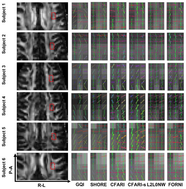
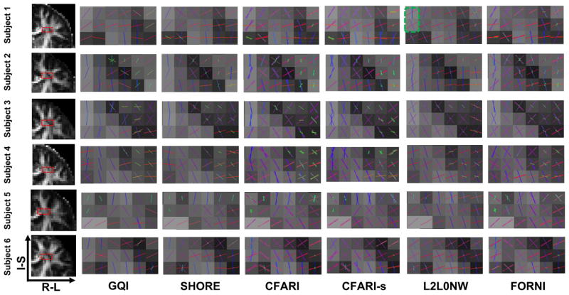
We highlight two regions for evaluation of the results on the six subjects: the crossing region of the superior longitudinal fasciculus (SLF) and the lateral corpus callosum (CC) in the axial view (Figure 13) and the crossing region of the lateral CC and the corticospinal tract (CST) in the coronal view (Figure 14). The results are shown with FA images in the left column. Compared to GQI, SHORE, CFARI, and CFARI-s, both L2L0NW and FORNI produces smooth FO estimation results and better identifies the crossing patterns in all cases. However, we note that in the region containing highly curved parts of the superior CC, for example, the one highlighted by the green box on Subject 1 in Figure 14, L2L0NW does not generate the FOs that correspond to the pathway of the superior CC. The effects of these kinds of errors will be better illustrated below in the fiber tracking results of Figures 15 and 16.
Figure 13.
FO estimation on brain dMRI (overlaid on the FA map) for all six subjects, which is focused on the crossing of SLF and the lateral CC (axial view). The FA image and the focused region are shown in the left column.
Figure 14.
FO estimation on brain dMRI (overlaid on the FA map) for all six subjects, which is focused on the crossing of the lateral CC and CST (coronal view). The FA image and the focused region are shown in the left column. Note the region highlighted by the green box where L2L0NW does not produces FOs that correspond to the geometry of the superior CC.
Figure 15.
A representative result (Subject 1) of fiber tracking using the INFACT tracking (Landman et al., 2012) overlaid on the FA map in the coronal view. The seeding region is represented as the yellow volume. Note the highlighted region where more lateral CC fiber streamlines were tracked using FOs computed by FORNI than GQI, SHORE, CFARI, and CFARI-s. The visualization was created in TrackVis (Wang et al., 2007).
Figure 16.
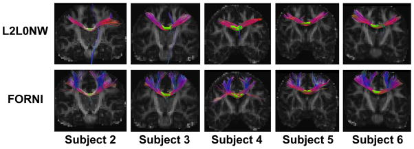
Fiber tracking results seeded in CC on Subjects 2–6 using L2L0NW and FORNI FOs. The seeding ROIs are indicated by the yellow volumes. The visualization was created in Track-Vis (Wang et al., 2007).
To further validate FORNI and compare it with the competing methods we used the INFACT algorithm (Landman et al., 2012) to carry out fiber tracking on the results of each algorithm. INFACT is a deterministic streamlining algorithm which extends the FACT algorithm (Mori et al., 1999) to our case where there are multiple FOs per voxel. We used an FA threshold of 0.15 and a turning angle threshold of 40°, which are common settings for tractography (Wahl et al., 2007; Glasser and Rilling, 2008; Kaplan et al., 2010). The seeds were placed in the noncrossing region of CC. A representative case (Subject 1) is shown in Figure 15, where the FORNI result can be compared to the results of GQI, SHORE, CFARI, CFARI-s, and L2L0NW. Here each segment of the fiber streamlines is color-coded by the standard DTI color scheme (red: left–right; green: front–back; and blue: up–down) (Pajevic and Pierpaoli, 1999). It can be seen that the lateral CC fiber streamlines are tracked better using FOs estimated by FORNI than GQI, SHORE, CFARI, and CFARI-s. In L2L0NW results, although the lateral CC is also well tracked, the superior CC is mostly missing, which is consistent with the FO estimation highlighted by the green box in Figure 14. This missing of the superior CC also exists in the other subjects, which is shown in Figure 16. Here, we applied fiber tracking using FORNI and L2L0NW FOs on the other five subjects with seeds placed in CC. We can see that FORNI is able to produce both superior and lateral CC but L2L0NW misses the superior CC.
4. Discussion
FORNI uses weighted ℓ1-norm regularization as in the FIEBR algorithm (Ye et al., 2015a), but the key ideas are very different between the two algorithms. First, the prior directions/likely FOs at each voxel are determined very differently. In Ye et al. (2015a), the prior directions are calculated based on the anatomical information of known tracts and it is aimed at resolving crossing fibers with a very limited number of gradient directions (around 12). Its performance could be affected by prior direction inaccuracies, for example, caused by inaccurate localization of tracts using registration. In the results in Figure 12 we can see that FIEBR can miss the crossing patterns due to the inaccurate specification of anatomical priors. In the proposed method no anatomical information is required, and the purpose is to improve FO estimation by incorporating spatial coherence of FOs. Second, the FOs are estimated at each voxel independently in Ye et al. (2015a) and no interaction between voxels is encoded while the proposed method jointly estimates the FOs in all voxels due to the interaction.
The L2L0NW algorithm (Auría et al., 2015a) also uses weighted ℓ1-norm to model the interaction between neighbors to enforce spatial regularization in its objective function. However, the motivation and the actual determination of the weighting are quite different between L2L0NW and FORNI. First, our method was motivated by the framework developed in Ye et al. (2015a), where the weighted ℓ1-norm is derived in a maximum a posteriori framework and is a consequence of modeling the prior density with a Laplace distribution and a term that encourages basis directions close to certain prior directions. The L2L0NW algorithm is motivated by the iterative reweighting scheme that seeks to better solve the ℓ0-norm minimization problem. Second, the weighting is determined differently. L2L0NW directly uses all the neighbor information in the weighting, and a neighbor FO has no influence on directions farther than 15° and uniform influence on directions within 15°. For a region with a highly curved tract, for example, the turning of the superior CC in Figure 14, it is possible that the desired FO is more than 15° away from its neighbor FOs and is not sufficiently encouraged. In FORNI, we process the information in the neighbors and extract likely FOs, and the weight decreases as the directions are closer to likely FOs. This strategy avoids the cutoff effect when a threshold of 15° is used in Auría et al. (2015a). In addition, we have used a voxel similarity term to avoid leakage of FOs, where the existence of undesired FOs at a voxel is a result of the impact of the FOs similar to the undesired ones in its neighbors. The voxel similarity puts higher weights on more similar neighbors and ensures anisotropic FO spatial consistency. This is especially important at tract boundaries and highly curved regions of tracts to suppress the influence of undesired FOs. As seen in the phantom experiment (Figure 8) and the brain dMRI results (Figure 14), L2L0NW can have leaking FOs at tract boundaries and miss the FOs of the curved superior CC, respectively, but this is avoided in FORNI.
A possible limitation of using the tensor distance in the voxel similarity is that at the boundary of the noncrossing part of a tract and its crossing part, the information in the noncrossing neighbors does not influence the current voxel as much as the crossing neighbors. It may be interesting to allow greater influence of noncrossing voxels on the crossing voxels that belong to the same tract while maintaining the avoidance of leaking of the FOs belonging to a different tract from the crossing voxels to noncrossing voxels.
In FORNI, the interaction between neighbors are decoupled using a BCD strategy. If a different update order of the voxels were used, the results of each iteration could be different. However, because multiple iterations are applied, the final results are expected to be very similar even if the update order is changed. But it would be interesting to explore adaptive sweeping patterns, such as Li and Osher (2009), so that the optimization is less dependent on the voxel order.
Instead of enforcing pairwise similarity between neighbor voxels, FORNI explicitly models neighbor FO information in the FO estimation by placing different penalties on the basis. Yet it is possible to combine the pairwise similarity with FORNI. For example, a straightforward improvement could be adding post-smoothing of FOs, such as Sigurdsson and Prince (2014), to the FORNI results. Indeed, the FORNI processing and the post-smoothing could be performed alternately with many iterations. These alternating iterative steps could actually correspond to the optimization of some unknown form of objective functions, which can be explored by future work to develop more powerful FO estimation algorithms.
Besides the directional information of FOs, the microstructural property has also been a quantity of interest computed from dMRI (Zhang et al., 2012; Daducci et al., 2015; Alexander et al., 2010; Auría et al., 2015b), which quantifies the tissue structure at mesoscale (Reisert et al., 2014), and recent work has further explored joint estimation of the microstructural characteristics and FOs (Girard et al., 2015). Among these works, Daducci et al. (2015) and Auría et al. (2015b) reformulate the estimation of microstructural properties by using a dictionary. Using this reformulation, it is possible to extend our framework to incorporate the estimation of the tissue organization, which could be improved by the incorporation of spatial smoothness.
At higher b-values, the diffusion is not Gaussian due to the restriction effects (Cohen and Assaf, 2002). Thus, there can be model inaccuracies caused by using the tensor basis. The sparsity and spatial regularization enforced by weighted ℓ1-norm terms could alleviate the issue. And it is possible to use the extension where microstructural properties are jointly estimated with FOs to account for the slow diffusing components.
5. Summary and Conclusion
In this work, we have proposed FORNI, an FO estimation algorithm that uses neighborhood information. A fixed tensor basis is used to represent the diffusion signals. To ensure spatial coherence, the directional information in the neighbors is explicitly modeled in weighted ℓ1-norm regularization terms. The resulting objective function is optimized using a BCD strategy and a parallelization approach to speeding up processing is presented. The proposed method was applied to a digital crossing phantom, ex vivo tongue dMRI data, and in vivo brain dMRI data. The results demonstrate that the proposed method is able to use neighborhood information to improve FO estimation.
Highlights.
We estimate fiber orientations (FOs) with the enforcement of spatial coherence.
Interaction between neighboring FOs is encoded in weighted l1 norm regularization.
Qualitative and quantitative validation was performed on simulated and real data.
The method reduces the effect of noise and improves the estimation of crossing FOs.
Acknowledgments
This work is supported by NIH/NINDS 5R01NS056307 and NIH/NINDS 1R21NS082891.
Appendix A. Optimization of the Weighted ℓ1-norm Regularized Least Squares Problem
In Eq. (17) the diagonal entries of (diagonal matrix) are given by (see Eq. (9))
| (A.1) |
Here, represents the p-th likely FO for voxel m at iteration t and is to be specified, and is the number of likely FOs for voxel m at iteration t. Eq. (17) explicitly acknowledges the fact that at time t, the estimate of fm uses information from voxels that have already been updated at time t as well as information from voxels that were updated at the previous time t − 1. (This is a Gauss-Seidel rather than a Jacobi update strategy.) Using this fact, the computed aggregate basis-neighbor similarity function for voxel m at time t is
| (A.2) |
where 𝟙 is an indicator function providing a shorthand notation to specify whether FOs at time t or t−1 are being used. The likely FOs at time t are then computed according to Eq. (14). With these definitions, Eq. (17) is fully specified.
Eq. (17) is a weighted ℓ1-norm regularized least squares problem which can be converted to an ℓ1-norm regularized least squares problem. First, we define a new variable . Since is a diagonal matrix and is invertible and . Then, by defining , we have
| (A.3) |
which we solve using the efficient optimization method for compressed sensing reported in Kim et al. (2007). The mixture fractions can be estimated as
| (A.4) |
Footnotes
Publisher's Disclaimer: This is a PDF file of an unedited manuscript that has been accepted for publication. As a service to our customers we are providing this early version of the manuscript. The manuscript will undergo copyediting, typesetting, and review of the resulting proof before it is published in its final citable form. Please note that during the production process errors may be discovered which could affect the content, and all legal disclaimers that apply to the journal pertain.
References
- Alexander DC, Hubbard PL, Hall MG, Moore EA, Ptito M, Parker GJ, Dyrby TB. Orientationally invariant indices of axon diameter and density from diffusion MRI. Neuro Image. 2010;52:1374–1389. doi: 10.1016/j.neuroimage.2010.05.043. [DOI] [PubMed] [Google Scholar]
- Aranda R, Rivera M, Ramirez-Manzanares A. A flocking based method for brain tractography. Medical Image Analysis. 2014;18:515–530. doi: 10.1016/j.media.2014.01.009. [DOI] [PubMed] [Google Scholar]
- Arsigny V, Fillard P, Pennec X, Ayache N. Log-Euclidean metrics for fast and simple calculus on diffusion tensors. Magnetic Resonance in Medicine. 2006;56:411–421. doi: 10.1002/mrm.20965. [DOI] [PubMed] [Google Scholar]
- Auría A, Daducci A, Thiran JP, Wiaux Y. Structured sparsity for spatially coherent fibre orientation estimation in diffusion MRI. Neuro Image. 2015a;115:245–255. doi: 10.1016/j.neuroimage.2015.04.049. [DOI] [PubMed] [Google Scholar]
- Auría A, Romascano DPR, Canales-Rodriguez E, Wiaux Y, Dirby TB, Alexander D, Thiran JP, Daducci A. Accelerated microstructure imaging via convex optimisation for regions with multiple fibres (AMICOx). IEEE International Conference on Image Processing; 2015; IEEE; 2015b. pp. 1673–1676. [Google Scholar]
- Basser PJ, Mattiello J, LeBihan D. MR diffusion tensor spectroscopy and imaging. Biophysical Journal. 1994;66:259–267. doi: 10.1016/S0006-3495(94)80775-1. [DOI] [PMC free article] [PubMed] [Google Scholar]
- Basser PJ, Pajevic S, Pierpaoli C, Duda J, Aldroubi A. In vivo fiber tractography using DT-MRI data. Magnetic Resonance in Medicine. 2000;44:625–632. doi: 10.1002/1522-2594(200010)44:4<625::AID-MRM17>3.0.CO;2-O. http://dx.doi.org/10.1002/1522-2594(200010)44:4<625::AID-MRM17>3.0.CO;2-O. [DOI] [PubMed] [Google Scholar]
- Bazin PL, Ye C, Bogovic JA, Shiee N, Reich DS, Prince JL, Pham DL. Direct segmentation of the major white matter tracts in diffusion tensor images. Neuro Image. 2011;58:458–468. doi: 10.1016/j.neuroimage.2011.06.020. [DOI] [PMC free article] [PubMed] [Google Scholar]
- Becker S, Tabelow K, Mohammadi S, Weiskopf N, Polzehl J. Adaptive smoothing of multi-shell diffusion weighted magnetic resonance data by msPOAS. Neuro Image. 2014;95:90–105. doi: 10.1016/j.neuroimage.2014.03.053. [DOI] [PMC free article] [PubMed] [Google Scholar]
- Behrens TEJ, Berg HJ, Jbabdi S, Rushworth MFS, Woolrich MW. Probabilistic diffusion tractography with multiple fibre orientations: What can we gain? Neuro Image. 2007;34:144–155. doi: 10.1016/j.neuroimage.2006.09.018. [DOI] [PMC free article] [PubMed] [Google Scholar]
- Bertsekas DP. Nonlinear Programming. 2. Athena Scientific; 1999. [Google Scholar]
- Bilgic B, Setsompop K, Cohen-Adad J, Yendiki A, Wald LL, Adalsteinsson E. Accelerated diffusion spectrum imaging with compressed sensing using adaptive dictionaries. Magnetic Resonance in Medicine. 2012;68:1747–1754. doi: 10.1002/mrm.24505. [DOI] [PMC free article] [PubMed] [Google Scholar]
- Cheng J, Deriche R, Jiang T, Shen D, Yap PT. Non-Negative Spherical Deconvolution (NNSD) for estimation of fiber Orientation Distribution Function in single-/multi-shell diffusion MRI. Neuro Image. 2014;101:750–764. doi: 10.1016/j.neuroimage.2014.07.062. [DOI] [PMC free article] [PubMed] [Google Scholar]
- Cheng J, Jiang T, Deriche R. Theoretical analysis and practical insights on EAP estimation via a unified HARDI framework. MICCAI Workshop on Computational Diffusion MRI (CDMRI).2011. [Google Scholar]
- Cheng P, Magnotta VA, Wu D, Nopoulos P, Moser DJ, Paulsen J, Jorge R, Andreasen NC. Evaluation of the GTRACT diffusion tensor tractography algorithm: a validation and reliability study. Neuro Image. 2006;31:1075–1085. doi: 10.1016/j.neuroimage.2006.01.028. [DOI] [PubMed] [Google Scholar]
- Cohen Y, Assaf Y. High b-value q-space analyzed diffusion-weighted MRS and MRI in neuronal tissues–a technical review. NMR in Biomedicine. 2002;15:516–542. doi: 10.1002/nbm.778. [DOI] [PubMed] [Google Scholar]
- Daducci A, Canales-Rodríguez EJ, Zhang H, Dyrby TB, Alexander DC, Thiran JP. Accelerated Microstructure Imaging via Convex Optimization (AMICO) from diffusion MRI data. Neuro Image. 2015;105:32–44. doi: 10.1016/j.neuroimage.2014.10.026. [DOI] [PubMed] [Google Scholar]
- Daducci A, Van De Ville D, Thiran JP, Wiaux Y. Sparse regularization for fiber ODF reconstruction: From the suboptimality of ℓ2 and ℓ1 priors to ℓ0. Medical Image Analysis. 2014;18:820–833. doi: 10.1016/j.media.2014.01.011. [DOI] [PubMed] [Google Scholar]
- Descoteaux M, Angelino E, Fitzgibbons S, Deriche R. Regularized, fast, and robust analytical q-ball imaging. Magnetic Resonance in Medicine. 2007;58:497–510. doi: 10.1002/mrm.21277. [DOI] [PubMed] [Google Scholar]
- Duits R, Franken E. Left-invariant diffusions on the space of positions and orientations and their application to crossing-preserving smoothing of HARDI images. International Journal of Computer Vision. 2011;92:231–264. [Google Scholar]
- Garyfallidis E, Brett M, Amirbekian B, Rokem A, Van Der Walt S, Descoteaux M, Nimmo-Smith I, Contributors D. Dipy, a library for the analysis of diffusion MRI data. Frontiers in Neuroinformatics. 2014;8:1–17. doi: 10.3389/fninf.2014.00008. [DOI] [PMC free article] [PubMed] [Google Scholar]
- Girard G, Fick R, Descoteaux M, Deriche R, Wassermann D. Information Processing in Medical Imaging. Springer; 2015. Axtract: microstructure-driven tractography based on the ensemble average propagator; pp. 675–686. [DOI] [PubMed] [Google Scholar]
- Glasser MF, Rilling JK. DTI tractography of the human brain’s language pathways. Cerebral Cortex. 2008;18:2471–2482. doi: 10.1093/cercor/bhn011. [DOI] [PubMed] [Google Scholar]
- Hess CP, Mukherjee P, Han ET, Xu D, Vigneron DB. Q-ball reconstruction of multimodal fiber orientations using the spherical harmonic basis. Magnetic Resonance in Medicine. 2006;56:104–117. doi: 10.1002/mrm.20931. http://dx.doi.org/10.1002/mrm.20931. [DOI] [PubMed] [Google Scholar]
- Jenkinson M, Beckmann CF, Behrens TEJ, Woolrich MW, Smith SM. FSL. Neuro Image. 2012;62:782–790. doi: 10.1016/j.neuroimage.2011.09.015. [DOI] [PubMed] [Google Scholar]
- Jeurissen B, Tournier JD, Dhollander T, Connelly A, Sijbers J. Multi-tissue constrained spherical deconvolution for improved analysis of multi-shell diffusion MRI data. Neuro Image. 2014;103:411–426. doi: 10.1016/j.neuroimage.2014.07.061. [DOI] [PubMed] [Google Scholar]
- Jian B, Vemuri BC. A unified computational framework for deconvolution to reconstruct multiple fibers from diffusion weighted MRI. IEEE Transactions on Medical Imaging. 2007;26:1464–1471. doi: 10.1109/TMI.2007.907552. [DOI] [PMC free article] [PubMed] [Google Scholar]
- Johansen-Berg H, Behrens TEJ. Diffusion MRI: from quantitative measurement to in vivo neuroanatomy. Academic Press; 2013. [Google Scholar]
- Kaplan E, Naeser MA, Martin PI, Ho M, Wang Y, Baker E, Pascual-Leone A. Horizontal portion of arcuate fasciculus fibers track to pars opercularis, not pars triangularis, in right and left hemispheres: a DTI study. Neuro Image. 2010;52:436–444. doi: 10.1016/j.neuroimage.2010.04.247. [DOI] [PMC free article] [PubMed] [Google Scholar]
- Kim SJ, Koh K, Lustig M, Boyd S. An efficient method for compressed sensing. IEEE International Conference on Image Processing; 2007. pp. 117–120. [Google Scholar]
- Landman BA, Bogovic JA, Wan H, ElShahaby FEZ, Bazin PL, Prince JL. Resolution of crossing fibers with constrained compressed sensing using diffusion tensor MRI. Neuro Image. 2012;59:2175–2186. doi: 10.1016/j.neuroimage.2011.10.011. [DOI] [PMC free article] [PubMed] [Google Scholar]
- Landman BA, Farrell JAD, Patel NL, Mori S, Prince JL. DTI fiber tracking: the importance of adjusting DTI gradient tables for motion correction. CATNAP - a tool to simplify and accelerate DTI analysis. Proc. Org Human Brain Mapping 13th Annual Meeting.2007. [Google Scholar]
- Li Y, Osher S. Coordinate descent optimization for ℓ1 minimization with application to compressed sensing; a greedy algorithm. Inverse Problems and Imaging. 2009;3:487–503. [Google Scholar]
- Liu X, Yuan Z, Guo Z, Xu D. A localized Richardson–Lucy algorithm for fiber orientation estimation in high angular resolution diffusion imaging. Medical Physics. 2015;42:2524–2539. doi: 10.1118/1.4917082. [DOI] [PubMed] [Google Scholar]
- Lucas BC, Bogovic JA, Carass A, Bazin PL, Prince JL, Pham DL, Landman BA. The Java image science toolkit (JIST) for rapid prototyping and publishing of neuroimaging software. Neuroinformatics. 2010;8:5–17. doi: 10.1007/s12021-009-9061-2. [DOI] [PMC free article] [PubMed] [Google Scholar]
- Merlet S, Caruyer E, Deriche R. Medical Image Computing and Computer- Assisted Intervention–MICCAI 2012. Springer; 2012. Parametric dictionary learning for modeling eap and odf in diffusion MRI; pp. 10–17. [DOI] [PubMed] [Google Scholar]
- Merlet SL, Deriche R. Continuous diffusion signal, EAP and ODF estimation via Compressive Sensing in diffusion MRI. Medical Image Analysis. 2013;17:556–572. doi: 10.1016/j.media.2013.02.010. [DOI] [PubMed] [Google Scholar]
- Michailovich O, Rathi Y, Dolui S. Spatially regularized compressed sensing for high angular resolution diffusion imaging. IEEE Transactions on Medical Imaging. 2011;30:1100–1115. doi: 10.1109/TMI.2011.2142189. [DOI] [PMC free article] [PubMed] [Google Scholar]
- Mori S, Crain BJ, Chacko VP, Van Zijl P. Three-dimensional tracking of axonal projections in the brain by magnetic resonance imaging. Annals of Neurology. 1999;45:265–269. doi: 10.1002/1531-8249(199902)45:2<265::aid-ana21>3.0.co;2-3. [DOI] [PubMed] [Google Scholar]
- Nazem-Zadeh MR, Davoodi-Bojd E, Soltanian-Zadeh H. Atlas-based fiber bundle segmentation using principal diffusion directions and spherical harmonic coefficients. Neuro Image. 2011;54:S146–S164. doi: 10.1016/j.neuroimage.2010.09.035. [DOI] [PubMed] [Google Scholar]
- Özarslan E, Shepherd TM, Vemuri BC, Blackband SJ, Mareci TH. Resolution of complex tissue microarchitecture using the diffusion orientation transform (DOT) Neuro Image. 2006;31:1086–1103. doi: 10.1016/j.neuroimage.2006.01.024. [DOI] [PubMed] [Google Scholar]
- Pajevic S, Pierpaoli C. Color schemes to represent the orientation of anisotropic tissues from diffusion tensor data: application to white matter fiber tract mapping in the human brain. Magnetic Resonance in Medicine. 1999;42:526–540. [PubMed] [Google Scholar]
- Peled S, Friman O, Jolesz F, Westin CF. Geometrically constrained two-tensor model for crossing tracts in DWI. Magnetic Resonance Imaging. 2006;24:1263–1270. doi: 10.1016/j.mri.2006.07.009. [DOI] [PMC free article] [PubMed] [Google Scholar]
- Pickalov V, Basser PJ. 3-D tomographic reconstruction of the average propagator from MRI data. 3rd IEEE International Symposium on Biomedical Imaging: Nano to Macro; IEEE; 2006. pp. 710–713. [Google Scholar]
- Qazi AA, Radmanesh A, O’Donnell L, Kindlmann G, Peled S, Whalen S, Westin CF, Golby AJ. Resolving crossings in the corticospinal tract by two-tensor streamline tractography: Method and clinical assessment using fMRI. Neuro Image. 2009;47:98–106. doi: 10.1016/j.neuroimage.2008.06.034. [DOI] [PMC free article] [PubMed] [Google Scholar]
- Ramirez-Manzanares A, Rivera M, Vemuri BC, Carney P, Mareci T. Diffusion basis functions decomposition for estimating white matter intravoxel fiber geometry. IEEE Transactions on Medical Imaging. 2007;26:1091–1102. doi: 10.1109/TMI.2007.900461. [DOI] [PubMed] [Google Scholar]
- Rathi Y, Michailovich O, Laun F, Setsompop K, Grant PE, Westin CF. Multi-shell diffusion signal recovery from sparse measurements. Medical Image Analysis. 2014;18:1143–1156. doi: 10.1016/j.media.2014.06.003. [DOI] [PMC free article] [PubMed] [Google Scholar]
- Reisert M, Kiselev V, Dihtal B, Kellner E, Novikov D. Medical Image Computing and Computer-Assisted Intervention–MICCAI 2014. Springer; 2014. MesoFT: Unifying diffusion modelling and fiber tracking; pp. 201–208. [DOI] [PMC free article] [PubMed] [Google Scholar]
- Reisert M, Kiselev VG. Fiber continuity: An anisotropic prior for ODF estimation. IEEE Transactions on Medical Imaging. 2011;30:1274–1283. doi: 10.1109/TMI.2011.2112769. [DOI] [PubMed] [Google Scholar]
- Reisert M, Mader I, Anastasopoulos C, Weigel M, Schnell S, Kiselev V. Global fiber reconstruction becomes practical. Neuro Image. 2011;54:955–962. doi: 10.1016/j.neuroimage.2010.09.016. [DOI] [PubMed] [Google Scholar]
- Sigurdsson GA, Prince JL. Smoothing fields of weighted collections with applications to diffusion MRI processing. SPIE Medical Imaging. 2014:90342D–90342D. doi: 10.1117/12.2043959. [DOI] [PMC free article] [PubMed] [Google Scholar]
- Stejskal EO, Tanner JE. Spin diffusion measurements: spin echoes in the presence of a time-dependent field gradient. The Journal of Chemical Physics. 1965;42:288. [Google Scholar]
- Tournier J, Calamante F, Connelly A. A robust spherical deconvolution method for the analysis of low SNR or low angular resolution diffusion data. International Society for Magnetic Resonance in Medicine. 2013:0772. [Google Scholar]
- Tournier JD, Calamante F, Connelly A. Robust determination of the fibre orientation distribution in diffusion MRI: Non-negativity constrained super-resolved spherical deconvolution. Neuro Image. 2007;35:1459–1472. doi: 10.1016/j.neuroimage.2007.02.016. [DOI] [PubMed] [Google Scholar]
- Tournier JD, Calamante F, Gadian DG, Connelly A. Direct estimation of the fiber orientation density function from diffusion-weighted MRI data using spherical deconvolution. Neuro Image. 2004;23:1176–1185. doi: 10.1016/j.neuroimage.2004.07.037. [DOI] [PubMed] [Google Scholar]
- Tuch DS. Q-ball imaging. Magnetic Resonance in Medicine. 2004;52:1358–1372. doi: 10.1002/mrm.20279. http://dx.doi.org/10.1002/mrm.20279. [DOI] [PubMed] [Google Scholar]
- Tuch DS, Reese TG, Wiegell MR, Makris N, Belliveau JW, Wedeen VJ. High angular resolution diffusion imaging reveals intravoxel white matter fiber heterogeneity. Magnetic Resonance in Medicine. 2002;48:577–582. doi: 10.1002/mrm.10268. http://dx.doi.org/10.1002/mrm.10268. [DOI] [PubMed] [Google Scholar]
- Wahl M, Lauterbach-Soon B, Hattingen E, Jung P, Singer O, Volz S, Klein JC, Steinmetz H, Ziemann U. Human motor corpus callosum: topography, somatotopy, and link between microstructure and function. The Journal of Neuroscience. 2007;27:12132–12138. doi: 10.1523/JNEUROSCI.2320-07.2007. [DOI] [PMC free article] [PubMed] [Google Scholar]
- Wang R, Benner T, Sorensen AG, Wedeen VJ. Diffusion toolkit: a software package for diffusion imaging data processing and tractography. Proc Intl Soc Mag Reson Med. 2007:3720. [Google Scholar]
- Wedeen VJ, Hagmann P, Tseng WYI, Reese TG, Weisskoff RM. Mapping complex tissue architecture with diffusion spectrum magnetic resonance imaging. Magnetic Resonance in Medicine. 2005;54:1377–1386. doi: 10.1002/mrm.20642. http://dx.doi.org/10.1002/mrm.20642. [DOI] [PubMed] [Google Scholar]
- Wedeen VJ, Wang R, Schmahmann JD, Benner T, Tseng W, Dai G, Pandya D, Hagmann P, D’Arceuil H, de Crespigny AJ. Diffusion spectrum magnetic resonance imaging (DSI) tractography of crossing fibers. Neuro Image. 2008;41:1267–1277. doi: 10.1016/j.neuroimage.2008.03.036. [DOI] [PubMed] [Google Scholar]
- Ye C, Carass A, Murano E, Stone M, Prince JL. A Bayesian approach to distinguishing interdigitated muscles in the tongue from limited diffusion weighted imaging, in: Bayesian and grAphical Models for Biomedical Imaging. Springer. volume 8677 of. Lecture Notes in Computer Science. 2014:13–24. doi: 10.1007/978-3-319-12289-2_2. [DOI] [PMC free article] [PubMed] [Google Scholar]
- Ye C, Murano E, Stone M, Prince JL. A Bayesian approach to distinguishing interdigitated tongue muscles from limited diffusion magnetic resonance imaging. Computerized Medical Imaging and Graphics. 2015a;45:63–74. doi: 10.1016/j.compmedimag.2015.07.005. http://www.sciencedirect.com/science/article/pii/S0895611115001032 http://dx.doi.org/10.1016/j.compmedimag.2015.07.005. [DOI] [PMC free article] [PubMed] [Google Scholar]
- Ye C, Yang Z, Ying SH, Prince JL. Segmentation of the cerebellar peduncles using a random forest classifier and a multi-object geometric deformable model: Application to spinocerebellar ataxia type 6. Neuroinformatics. 2015b;13:367–381. doi: 10.1007/s12021-015-9264-7. http://dx.doi.org/10.1007/s12021-015-9264-7. [DOI] [PMC free article] [PubMed] [Google Scholar]
- Ye C, Zhuo J, Gullapalli RP, Prince JL. Estimation of fiber orientations using neighborhood information. Computational Diffusion MRI: MICCAI Workshop; Munich, Germany. October 9th, 2015; Springer; 2016. pp. 87–96. [DOI] [PMC free article] [PubMed] [Google Scholar]
- Yeh FC, Wedeen V, Tseng WY. Generalized q-sampling imaging. IEEE Transactions on Medical Imaging. 2010;29:1626–1635. doi: 10.1109/TMI.2010.2045126. [DOI] [PubMed] [Google Scholar]
- Yendiki A, Panneck P, Srinivasan P, Stevens A, Zöllei L, Augustinack J, Wang R, Salat D, Ehrlich S, Behrens T, Jbabdi S, Gollub R, Fischl B. Automated probabilistic reconstruction of white-matter pathways in health and disease using an atlas of the underlying anatomy. Frontiers in Neuroinformatics. 2011;5:12–23. doi: 10.3389/fninf.2011.00023. [DOI] [PMC free article] [PubMed] [Google Scholar]
- Zhang H, Schneider T, Wheeler-Kingshott CA, Alexander DC. NODDI: practical in vivo neurite orientation dispersion and density imaging of the human brain. Neuro Image. 2012;61:1000–1016. doi: 10.1016/j.neuroimage.2012.03.072. [DOI] [PubMed] [Google Scholar]
- Zhou Q, Michailovich O, Rathi Y. Resolving complex fibre architecture by means of sparse spherical deconvolution in the presence of isotropic diffusion. SPIE Medical Imaging. 2014:903425–903425. [Google Scholar]


