Caffe con Troll: Shallow Ideas to Speed Up Deep Learning

Abstract

We present Caffe con Troll (CcT), a fully compatible end-to-end version of the popular framework Caffe with rebuilt internals. We built CcT to examine the performance characteristics of training and deploying general-purpose convolutional neural networks across different hardware architectures. We find that, by employing standard batching optimizations for CPU training, we achieve a 4.5× throughput improvement over Caffe on popular networks like CaffeNet. Moreover, with these improvements, the end-to-end training time for CNNs is directly proportional to the FLOPS delivered by the CPU, which enables us to efficiently train hybrid CPU-GPU systems for CNNs.

1. INTRODUCTION

Deep Learning using convolution neural networks (CNNs) is a hot topic in machine learning research and is the basis for a staggering number of consumer-facing data-driven applications, including those based on object recognition, voice recognition, and search [5,6,9,16]. Deep Learning is likely to be a major workload for future data analytics applications. Given the recent resurgence of CNNs, there have been few studies of CNNs from a data-systems perspective.

Database systems have a role here, as efficiency in runtime and cost are chief concerns for owners of these systems. In contrast to many analytics that are memory-bound [15], CNN calculations are often compute-bound. Thus, processor technology plays a key role in these systems. GPUs are a popular choice to support CNNs, as modern GPUs offer between 1.3 TFLOPS (NVIDIA GRID K520) and 4.29 TFLOPS (NVIDIA K40). However, GPUs are connected to host memory by a slow PCI-e interconnect. On the other hand, Microsoft's Project Adam argues that CPUs can deliver more cost-effective performance [4].¹ This debate is only going to get more interesting: the next generation of GPUs promise high-speed interconnection with host memory,² while Intel's current Haswell CPU can achieve 1.3T FLOPS on a single chip. Moreover, SIMD parallelism has doubled in each of the last four Intel CPU generations and is likely to continue.³ For users who cannot control the footprint of the data center, another issue is that Amazon's EC2 provides GPUs, but neither Azure nor Google Compute do. This motivates our study of CNN-based systems across different architectures.

To conduct our study, we forked Caffe, the most popular open-source CNN system, and rebuilt its internals to produce a system we call Caffe con Troll (CcT)⁴. CcT is a fully compatible end-to-end version of Caffe that matches Caffe's output on each layer, which is the unit of computation. As reported in the literature and confirmed by our experiments, the bottleneck layers are the so-called convolutional layers, which consume between 70-90% of execution time. Although we optimize all layers in CcT using essentially the same techniques, we focus on the tradeoff space for the convolutional layer on CPUs and GPUs.

The convolutional layer operates on batches of tensors. Currently, CcT studies one method of performing the convolution called lowering, which remaps the high-dimensional input tensors into a series of standard matrix multiplications. In turn, these matrix multiplications are executed using a BLAS-compatible library, such as OpenBLAS or Intel's MKL. Lowering is used in many state-of-the-art systems, including Caffe and CuDNN. Previous approaches picked a single lowering, but we find that there are at least three different ways to lay out (or block) the matrices in the lowering operation. Our study reveals that the optimal strategy depends on the ratio of input to output channels of the convolution, and that while this means that one lowering usually dominates the others, we offer experimental evidence of this fact and propose a simple automatic optimizer to pick the best lowering in the tradeoff space automatically. On popular networks, we find that the optimal lowering contributes around 20% of the execution time for a single layer, and 5% performance improvement for end-to-end execution.

More significantly, with some standard batching optimizations that are not employed in other systems, our study reveals that CPU systems are much faster than is often reported in the literature. Using a simple batching strategy, we achieve a 4.5× end-to-end speed improvement over Caffe on popular networks like CaffeNet, and up to an order of magnitude speedup for convolutional layers. Moreover, the end-to-end time is proportional to the FLOPS delivered by the CPU.

We build on this proportionality of the devices to create a hybrid CPU-GPU system. Typically, CNN systems are either GPU-based or CPU-based–but not both. And the debate has reached almost religious levels. Using CcT, we argue that one should use both CPUs and GPUs, simultaneously. CcT is the first hybrid system that uses both CPUs and GPUs on a single layer. We show that on the EC2 GPU instance, even with an underpowered, older 4-core CPU, we can achieve 20% higher throughput on a single convolutional layer. Thus these hybrid solutions may become more effective than homogeneous systems and open new questions in provisioning such CNN systems. Finally, on the newly announced Amazon EC2 instance with 4 GPUs we also show end-to-end speedups for 1 GPU + CPU of > 15% and speedups of > 3× using 4 GPUs.

2. CCT'S TRADEOFFS

We first describe the definition of a convolution operation and a technique called lowering, which is a popular way to implement the convolution operation. We describe three different lowering techniques.

A convolutional layer consumes a pair of order 3 tensors–the data $D\in {\mathbb{R}}^{n\times n\times d}$ and the kernel $K\in {\mathbb{R}}^{k\times k\times d}$. In AlexNet [9], n ∈ [13, 227], k ∈ [3, 11], and d ∈ [3, 384], The output is a 2D matrix $R\in {\mathbb{R}}^{m\times m}$ where m = n – k + 1 and each element R_r,c is defined as:

$$R_{r,c}=\sum _{i=1}^d\sum _{c^{\prime }=0}^{k-1}\sum _{r^{\prime }=0}^{k-1}{D}_{r+r^{\prime },c+c^{\prime },i}{K}_{r^{\prime },c^{\prime },i}$$ (1)

This is the standard image 2d-convolution with many kernels indexed by the third index of K. Like most other HPC kernels, a straightforward implementation of this operation is suboptimal. We transform the tensor problem into highly-optimized matrix multiplication kernels. The convolution layer takes as input a set of data tensors {D_i} and {K_j}, where we call b = |D_i| the batch size and o = |K_j| the number of output channels. We consider how to batch this computation below.

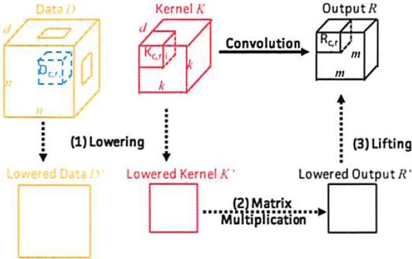
2.1 Lowering-based Convolution

As in Figure 1, there are three logical steps in the lowering process: (1) lowering, in which we transform 3D tensors D and K into 2D matrices D̂ and K̂; (2) multiply, in which we multiply D̂K̂ to get the the result R̂; and (3) lifting, in which we transform R̂ in back to a tensor representation of R.

Figure 1.

An illustration of the convolution operation and the commutative diagram of calculating convolution operations with lowering-based method.

Lowering Phase in which we construct the matrix D̂ and K̂. A value of K and D may appear more than once in the lowered matrices.

Multiply Phase in which we multiply D̂ and K̂ to create R̂ = D̂K̂.

Lifting Phase in which we map R̂ back to R.

Lowering Strategies

Different lowering strategies correspond to different ways to group the sum in Equation 1. Let $X\in {\mathbb{R}}^{5\times 7}$. First, we use zero-based indexing and array slice notation to describe these operations, i.e., Y = X[0 : 5, 3 : 5] indicates that $Y\in {\mathbb{R}}^{5\times 2}$ is a submatrix of X such that Y[i, j] = X[i, 3 + j] for i = 0, ..., 4 and j = 0, 1. We also use wildcards, i.e., Y = X[:, 3 : 5] = X[0 : 5, 3 : 5] since the first dimension of X is of size 5. We define Z = vec(Y) for $Z\in {\mathbb{R}}^{10}$ to be Z_5i+j = Y_i,j. We explore three choices: lowering more expensive than lifting, lifting more expensive than lowering, or a balance.

Type 1: Expensive Lowering

We create $\widehat{D}\in {\mathbb{R}}^{m^2\times k^{2}d}$ and $\widehat{K}\in {\mathbb{R}}^{k^{2}d}$ as follows for r, c ∈ 0, ..., m – 1:

$$\begin{array}{cc}\hfill \widehat{D}[cm+r,:]& =\mathrm{vec}\left(D[r:r+k,c:c+k,:]\right)\hfill \\ \hfill \widehat{K}& =\mathrm{vec}\left(K\right)\hfill \end{array}$$

We have $\widehat{R}=\widehat{D}\widehat{K}\in {\mathbb{R}}^{m^2\times 1}$ matrix, which is trivial to reshape to R. The lowering makes k² copies of K and D, but after the matrix multiply requires only trivial lifting.

Type 3: Expensive Lifting

We could trade lowering cost for lifting cost by simply starting with the sum over index i in Equation 1. That is, $\widehat{D}\in {\mathbb{R}}^{n^2\times d}$ and K̂ ∈ R^d×k2.

$$\begin{array}{cc}\hfill \widehat{D}[cn+r,:]=& \mathrm{vec}\left(D[r,c,:]\right)\hfill \\ \hfill \widehat{K}[:,ik+j]=& \mathrm{vec}\left(K[i,j,:]\right)\hfill \end{array}$$

for r, c ∈ 0, ..., n – 1 and i, j ∈ 0, ..., k – 1. Let $\widehat{R}=\widehat{D}\widehat{K}\in {\mathbb{R}}^{n^2\times k^2}$ then the lifting phase is:

$$R[r,c]=\sum _{i=0}^{k-1}\sum _{j=0}^{k-1}\widehat{R}[(c+j)n+r+i,ik+j]$$

In Type 3, the matrix multiply is on a smaller matrix, the lifting takes time Θ(m²k²), which is more expensive than the Θ(m²) time for Expensive Lowering.

Type 2: Balanced

Lowerings of type 1 and 3 represent two extremes of the spectrum, in which the k² blowup is either in the lowering phase or the lifting phase. A natural middle point in this spectrum balances the expense on both lowering and lifting, which we call balanced. Here $\widehat{D}\in {\mathbb{R}}^{n^2\times k+d}$ and $\widehat{K}\in {\mathbb{R}}^{k+d\times k}$.

$$\begin{array}{cc}\hfill \widehat{D}[cn+r,:]& =\mathrm{vec}\left(D[r,c:c+k,:]\right)\hfill \\ \hfill \widehat{K}[:,i]& =\mathrm{vec}\left(K[i,:,:]\right)\hfill \end{array}$$

Let $\widehat{R}=\widehat{D}\widehat{K}\in {\mathbb{R}}^{n^2\times k}$, then the lifting phase is:

$$R[r,c]=\sum _{j=0}^{k-1}\widehat{R}[cn+r+j,j]$$

Lowering and lifting take Θ(m²k) time and space which sits squarely between the other two approaches. As expected, the matrix multiplication is of an intermediate cost. We study the tradeoffs empirically in Appendix A.

Fusion

Conceptually, it is straightforward to fuse all three steps to avoid the materialization cost of lowering; this requires rewriting BLAS kernels. We developed such a kernel for CcT, and our preliminary experiments indicate that it can improve performance by up to 60%. In this paper, we only report numbers without fusion, so we do not discuss this optimization further.

2.2 Batching Analysis

This section discusses how partitioning the batch into partitions and processing these batch partitions in parallel leads to significant speedups on the CPU. To accomplish this for convolution, the matrix we create in the lowering phase is b times larger than when images are processed one at a time.

First we study the memory footprint and performance related to how large a batch we execute in the CPU matrix multiplication (GEMM). Caffe uses a batch size of 1 for convolutions. This means that for each image, lowering and GEMM are done sequentially. This has the smallest possible memory footprint, as it only needs to maintain the lowered matrix of a single D_i in memory; on the other hand, a batch of size b takes b times more memory. As shown in Figure 2(c), for convolutional layers on a CPU, the difference in memory footprint between b = 1 and b = 256 is directly proportional to b. For devices with limited memory, such as GPUs, one might favor b = 1 over large batch sizes.

Figure 2.

The impact of batch size and number of threads (8 physical cores in total) on the GEMM kernel.

Computationally however, we find that b = 1 suffers from lower hardware efficiency. Figure 2(a,b) shows the speedup w.r.t. number of cores for different batch sizes. When the batch size is large (256) as shown in Figure 2(a), on a machine with 8 physical cores, we observe almost linear speedup up to 4 cores. We then vary the batch size in Figure 2(b) and plot the speedup (using 8 physical cores). We see that the smaller the batch size, the lower the speedup. When the batch size is 1, using 8 cores actually causes a 4× slowdown compared to using 1 core. The underlying reason is that the lowered data matrix, D̂, is ‘thinner’ when b = 1 than for higher batch sizes. Thinner matrices mean that possible partition sizes of the underlying algorithm are smaller, and the kernel is unable to optimize, for example the L2 and L3 caches cannot be filled during blocking optimizations. As a result, b = 1 is more likely memory-bandwidth-bound than higher batch sizes. This phenomenon is likely to be more severe when the GEMM kernel is executed with multiple threads. Hence, we advocate the simple strategy to batch as much as possible (as device memory permits). Note that this could mean processing an entire batch (of size b) at once with n threads used in GEMM, or partitioning the batch into p partitions of size b/p with n/p threads used in each GEMM. These are equivalent as this is exactly how BLAS parallelizes GEMM: by partitioning partition columns of B in A × B and allocating 1 thread per partition.

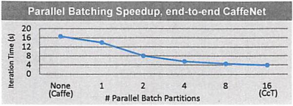
While such a batch partitioning strategy is equivalent in terms of GEMM, it is a coarse-grained way to perform lowering in parallel, and similar batch partitioning can be employed to parallelize all layers. Figure 3 shows the impact of batch partitioning on a full end-to-end CaffeNet on the EC2 c4.4xlarge instance with 16 physical cores. The batch size used is 256 images and the horizontal axis represents into how many parallel partitions CcT partitioned these 256 images. “None” indicates the default Caffe implementation, which for convolutions is that each image is processed serially (one at a time) and for other layers as a full batch (256 images). “1” indicates that all 256 images were processed together (for convolution layers, this means that lowering was performed on the entire batch of size 256 and then a single GEMM with 16 parallel threads was used to perform the entire convolution). For all other number of parallel partitions p, the 256 images were equally split into p partitions (for example if p = 2, two partitions of size 128). Layers were processed for each partition in parallel (one thread per partition), and then (so that for each data point shown all 16 threads are used during convolution), the GEMM is performed in parallel on each partition with 16/p threads per GEMM. For example the point “4” indicates 4 partitions of size 64, and during convolutions, lowering and GEMM (with 4 threads) was done in parallel for each of the 4 partitions.

Figure 3.

The impact of batching on the end-to-end execution time of CaffeNet, run with 256 images per mini-batch on an Amazon EC2 c4.4xlarge instance.

2.3 Scheduling Analysis

We currently only consider data parallelism within a layer (the model is shared). The key decision is what fraction of the input to send to each device. We use a simple heuristic: each device takes a fraction p of input in which p is the fraction of total FLOPS that this device contributes. So if a CPU has 1 TFLOPS and a GPU has 2 TFLOPS, we send 1/3 of the input to the CPU. In Appendix B, we find this simple heuristic is within 5% of the optimal performance.

3. EXPERIMENTS

We conduct an experimental evaluation of CcT.

3.1 Experiment Setup

To evaluate CcT, we compare it with Caffe, one of the most popular libraries for CNNs. We run both systems on the neural network architectures from CaffeNet (AlexNet), the default architecture for benchmarking. We compile both CcT and Caffe with GCC-4.8.2 and NVCC-6.5.12, and use OpenBLAS for CPU versions and the cuBLAS shipped with CUDA 6.5 for GPU versions.

3.2 End-to-end Performance

We run CcT and Caffe on ImageNet datasets with CaffeNet on a diverse set of EC2 machines as illustrated in Figure 4. Both systems take as input the same network configuration file that Caffe provides.⁵ Given the same random seed, CcT and Caffe generate the same output per layer (including the result of convolution, and the learned model) within a small tolerance. Thus, we concentrate on throughput. We run CcT and Caffe for 10 iterations and compare the output and model of each layer. We find that both systems produce the same output within 0.1% relative error. Thus, we focus our remaining experiments only on runtime performance.

Figure 4.

End-to-end performance comparison across different machines on CaffeNet. All numbers are normalized as the speedup over running Caffe's GPU version on g2.2xlarge instance ($0.47/hour).

Performance

To compare the performance between CcT and Caffe, we run all systems on different EC2 instances for 10 iterations, take the average, and report the time that each system spends for one iteration (256 images).⁶

We see from Figure 4(b) that on EC2's CPU instance (c4.4xlarge), which has a single-socket Haswell CPU with 8 physical cores. CcT outperforms Caffe by 4.5×. The speedup is mostly due to Caffe lowering single images at a time while CcT lowers with batching. Similar results were obtained on a two-socket CPU instance (c4.8xlarge). Both CcT and Caffe use only Lowering Type 1. We observed that Type 3 becomes faster than Type 1 as the ratio #input/#output channels increases, but this is only true of conv5 and the difference is small (see Appendix A).

Probably the most interesting comparison is CcT on a CPU instance to Caffe on a GPU instance. On the GPU instance, we find that Caffe is 1.86× faster than CcT running on 8 CPU cores, and slightly slower than CcT running on 16 CPU cores. We find that the GPU instance provides a peak ability of 1.3 TFLOPS, while the single-socket CPU instance provides 0.7 TFLOPS. The difference between the peak floating point operations corresponds to the performance difference between Caffe and CcT.

Price Analysis

We compare the price of running Caffe on a GPU instance and CcT on a CPU instance (c4.4xlarge) for the same number of iterations. We see that running on a CPU instance is 2.6× more expensive than a GPU instance given the difference in performance and the fact that the GPU instance is slightly cheaper than a CPU instance.⁷ However, this number is far smaller than one order of magnitude, which is typically associated to CPU-based Deep Learning. This suggests to us that, on other cloud services without GPU instances, e.g., Microsoft Azure and Google Compute, one can train a Deep Learning workload with a pure CPU version using CcT.

3.3 CPU/GPU Hybrid and Multi-GPU

We validate that using the CPUs on a GPU instance can accelerate purely CPU or GPU training. We first focus on the speed of running the convolution operation. We implement a GPU version of CcT and a hybrid version that, for each batch of images, runs a subset over GPU and others over CPU. We run both systems on the EC2 GPU instance, which has 4 Ivy Bridge CPU cores, and report the number in Figure 4(a). We run both system on the first convolutional layer in CaffeNet, both with grouping 1 (depth=48) and 2 (depth=96).

We see that CcT (GPU) achieves the same speed as Caffe, and that running CcT with both CPU and GPU provides significant benefit–CcT (CPU+GPU) with 85% batch run on GPU and 15% batch run on CPU is 20% faster than Caffe. The small CPU batch proportion is because the CPU cores on the GPU instance g2.2xlarge only provide 4× fewer peak FLOPS than the standalone CPU instance (c4.4xlarge), due to fewer cores and an older available instruction set (in fact, this CPU is even slower than a 2014 MacBook Pro with 4 Haswell cores). Therefore, we expect an even larger hybrid improvement on a GPU instance with a better CPU.

Finally, Figure 5 presents end-to-end AlexNet execution time on the EC2 g2.8xlarge instance, for 1 GPU, 1 GPU + CPU, and 4 GPUs. For 1 GPU, Caffe and CcT have the same execution time per iteration. Adding the CPU gives > 15% speedup, although we expect this number to increase with further optimizations. 4 GPUs currently give a speedup > 3×, although this too should approach 4× once CcT supports model parallelism for fully-connected layers.

Figure 5.

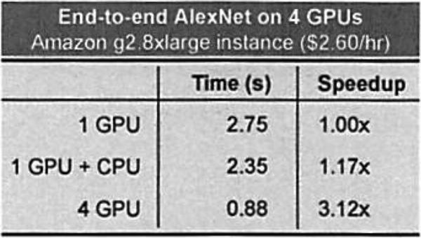
Speedup obtained in CcT with multiple GPUs.

4. RELATED WORK

We briefly describe previous studies which also focus on improving the efficiency of Deep Learning primitives. Although our contributions in this paper leverage decades of work in high-performance computing (specifically, the advancements in optimizing matrix multiplications [7, 14]), we omit discussion of this due to space constraints.

CNNs are computationally expensive, and optimizing CNN performance has become a well-studied problem in recent years. Popular libraries include Caffe [8], Theano [1], cuda-convnet2,⁸ and cuDNN [3]. To compute convolutions, many of these frameworks use lowering, an idea proposed by Chellapilla et al. [2] that takes advantage of highly-optimized BLAS libraries. Our work follows from this line of research, but we instead explore the tradeoffs between different types of lowerings, which has not been previously studied. Another approach for computing convolutions that has recently gained attention is to use the Fast Fourier Transform [12]. This work has also demonstrated a set of interesting performance tradeoffs based on the size of the input, and we hope to incorporate these additional optimizations in future work.

Automatic Optimization

A performance tradeoff arises when computing convolutions across a series of inputs. For example, Chetlur et al. [3] demonstrate that the performance of the convolution operation is parameterized by 11 dimensions; thus, optimizing the computation further is a “difficult task.” In this paper, we analyze this sophisticated tradeoff space in more detail; we find that a single ratio can be used to characterize all three lowering techniques. Recently, the Theano [1] library embraced the idea of building a so-called “meta-optimizer” in their Nov 2014 code release. This meta-optimizer would treat the various approaches to computing convolutions as black-box solvers, and would select the optimal approach for a given input. This idea is similar to our notion of an automatic optimizer; however, our intention is to understand the tradeoff space within a particular strategy, rather than relying on existing approaches.

Distributed Deep Learning

Distributed systems for Deep Learning is a popular topic including SINGA [13], Google's DistBelief [5], and Microsoft's Project Adam [4]. These efforts concentrate on two core challenges – scheduling across different nodes, and distributing model parameters across different nodes. A technique used in the above approaches is Hogwild! [10], which was designed for a single node and has since been extended to a distributed setting [11]. In the same spirit, our work focuses on improving CNN performance in the context of a single node. In future work, we also plan to study CNN training in the distributed setting, and we believe our efforts for the single-node case may lead to performance gains in these distributed settings.

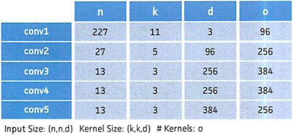
Figure 7.

The size of each convolution layer in AlexNet.

APPENDIX

A. STUDY OF LOWERING TRADEOFF

A.1 Empirical and Analytical Analysis

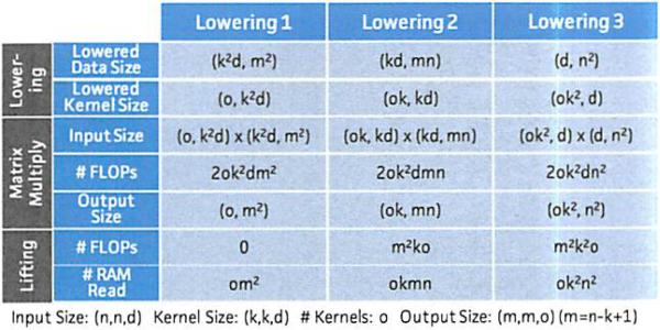
We summarize the tradeoff space analytically in Figure 6 and empirically in Figures 8 and 2. For matrix multiplication, we report the cost of OpenBLAS that is cubic to the input dimension. For simplicity of notation, we focus on analyzing the case that n is large enough such that the difference between m = n – k + 1 and n are secondary.

Figure 6.

Cost model of lowering strategies.

Figure 8.

Empirical tradeoffs of different lowering strategies.

(Analytical Analysis)

One key observation from Figure 6 is that lowering type 1 (resp. type 3) has the largest (resp. smallest) input size of lowered data and the smallest (resp. largest) output size after matrix multiplication. Lowering type 2 is in between. If we let m and n be constant, we can see that lowering type 1 involves a k² blowup on the data of size O(d), the number of input channels, and lowering type 2 involves a k² blowup on the data of size O(o), the number of output channels. The relative performance of the two strategies depends on the ratio of d and o.

(Empirical Analysis)

We validate our analytical cost model. In Figure 8(a,b), we vary d and o respectively with all other dimensions fixed. We see that each strategy performs differently as we vary d and o, and neither of them dominates the other. As one would expect, when the number of output channels (o) decreases, lowering type 3 outperforms lowering type 1 and vice versa. The difference in efficiency between the two approaches can be up to one order of magnitude.

We find that the relative performance of the different lowering strategies is determined by the ratio between the number of input channels and the number of output channels. Figure 8(c) demonstrates the relative performance between lowering type 1 and lowering type 3 w.r.t. the ratio between input channels and output channels while all other dimensions are fixed. We see that when the ratio increases (more input channels), type 3 outperforms type 1, and vice versa. While this allows us to choose the strategy optimally, on most current CNNs this ratio is within a narrow band. Hence, the lowering does not have a major impact on our performance.

B. CROSS-DEVICE SCHEDULING

We validate that our simple heuristic yields near-optimal scheduling results by estimating p, the fraction of total FLOPS that each device contributes. We follow the experiment protocol as in Section 3.3 but vary the ratio p as shown in Figure 9. Here, p denotes the fraction of jobs that run on the GPU. We see from Figure 9 that when p is too large or too small, the speedup of cross-device scheduling is less than 1; in essence, the GPU finishes early. Empirically, the optimal p is achieved at 83%. We also label the estimated p using our simple heuristic with the theoretical peak TFLOPS that the device could deliver, and find that it is within 5% of the optimal scheduling plan. We also tried to estimate the p using the empirical TFLOPS that each device gets, and find the result is similar; the speedup is still within 5% of the optimal p.

Figure 9.

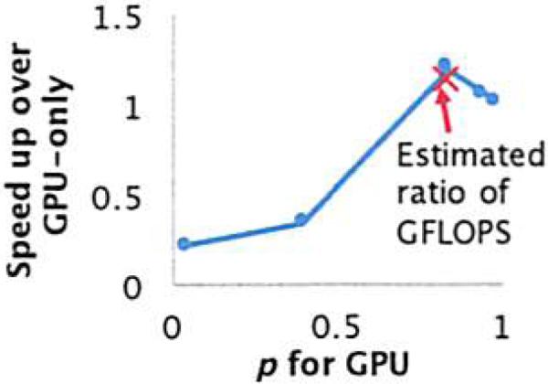
The Impact of Task Ratio p between GPU and CPU to Speed Up.

REFERENCES

- 1.Bergstra J, Breleux O, Bastien F, Lamblin P, Pascanu R, Desjardins G, Turian J, Warde-Farley D, Bengio Y. Theano: a CPU and GPU math expression compiler. SciPy. 2010 Jun; Oral Prcscntation. [Google Scholar]
- 2.Chellapilla K, et al. High performance convolutional neural networks for document processing. ICFHR. 2006 [Google Scholar]
- 3.Chetlur S, Woolley C, Vandermersch P, Cohen J, Tran J, Catanzaro B, Shelhamer E. cuDNN: Efficient Primitives for Deep Learning. ArXiv e-prints. 2014 [Google Scholar]
- 4.Chilimbi T, Suzue Y, Apacible J, Kalyanaraman K. Project adam: Building an efficient and scalable deep learning training system. OSDI. 2014 [Google Scholar]
- 5.Dean J, et al. Large scale distributed deep networks. NIPS. 2012 [Google Scholar]
- 6.Deng L, Yu D. Deep learning: Methods and applications. Foundations and Trends in Signal Processing. 2014 [Google Scholar]
- 7.Goto K, Van De Geijn R. High-performance implementation of the level-3 blas. ACM Trans. Math. Softw. 2008 [Google Scholar]
- 8.Jia Y, Shelhamer E, Donahue J, Karayev S, Long J, Girshick R, Guadarrama S, Darrell T. Caffe: Convolutional architecture for fast feature embedding. arXiv preprint arXiv. 2014;1408.5093 [Google Scholar]
- 9.Krizhevsky A, Sutskever I, Hinton GE. ImageNet classification with deep convolutional neural networks. NIPS. 2012 [Google Scholar]
- 10.Niu F, Recht B, Ré C. Wright SJ, editor. Hogwild!: A lock-frce approach to paral1elizing stochastic gradient descent. NIPS. 2011:693–701. [Google Scholar]
- l1.Noel C, Osindero S. Dogwi1d!: Distributed Hogwi1d for CPU & GPU. NIPS workshop on Distributed Machine Learning and Matrix Computations. 2014 [Google Scholar]
- 12.Vasilache N, Johnson J, Mathieu M, Chintala S, Piantino S, LeCun Y. Fast Convolutional Nets With fbfft: A GPU Performance Evaluation. ArXiv e-prints. 2014 Dec; [Google Scholar]
- 13.Wang W, Chen G, Dinh T, Gao J, Ooi B, Tan K. SINGA: A distributed system for deep learning. Technical report, NUS Tech Report. 2015 [Google Scholar]
- 14.Whaley RC, Dongarra JJ. Automatically tuned linear algebra software. SC. 1998 [Google Scholar]
- 15.Zhang C, Ré C. DimmWittcd: A study of main-memory statistical analytics. PVLDB. 2014 [Google Scholar]
- 16.Zhang X, LeCun Y. Text Understanding from Scratch. ArXiv e-prints. 2015 [Google Scholar]