Jumping across biomedical contexts using compressive data fusion

Abstract

Motivation: The rapid growth of diverse biological data allows us to consider interactions between a variety of objects, such as genes, chemicals, molecular signatures, diseases, pathways and environmental exposures. Often, any pair of objects—such as a gene and a disease—can be related in different ways, for example, directly via gene–disease associations or indirectly via functional annotations, chemicals and pathways. Different ways of relating these objects carry different semantic meanings. However, traditional methods disregard these semantics and thus cannot fully exploit their value in data modeling.

Results: We present Medusa, an approach to detect size-k modules of objects that, taken together, appear most significant to another set of objects. Medusa operates on large-scale collections of heterogeneous datasets and explicitly distinguishes between diverse data semantics. It advances research along two dimensions: it builds on collective matrix factorization to derive different semantics, and it formulates the growing of the modules as a submodular optimization program. Medusa is flexible in choosing or combining semantic meanings and provides theoretical guarantees about detection quality. In a systematic study on 310 complex diseases, we show the effectiveness of Medusa in associating genes with diseases and detecting disease modules. We demonstrate that in predicting gene–disease associations Medusa compares favorably to methods that ignore diverse semantic meanings. We find that the utility of different semantics depends on disease categories and that, overall, Medusa recovers disease modules more accurately when combining different semantics.

Availability and implementation: Source code is at http://github.com/marinkaz/medusa

Contact: marinka@cs.stanford.edu, blaz.zupan@fri.uni-lj.si

1 Introduction

In recent years, there is increasing evidence that gene–disease association prediction and disease module detection can benefit from integrative data analysis (Moreau and Tranchevent, 2012; Ritchie et al., 2015). Large-scale molecular biology data systems analyzed with integrative approaches are typically heterogeneous and contain objects of different types, such as genes, pathways, chemicals, disease symptoms and exposure measurements. These objects interconnect through multiple, most often pairwise, relations encoded in the data. Consider an example of such a data system from Figure 1 that contains 16 datasets (solid edges) and objects of 13 different types (nodes). For example, dataset $R^{2,7}$ encodes the clinical manifestations of diseases, whereas dataset $R^{5,3}$ describes associations of chemicals with biological processes and molecular functions. The ubiquity of complex data systems of this kind presents many unique opportunities and challenges for uncovering genotype–phenotype interactions, or, in general, interactions between any kind of objects.

Fig. 1.

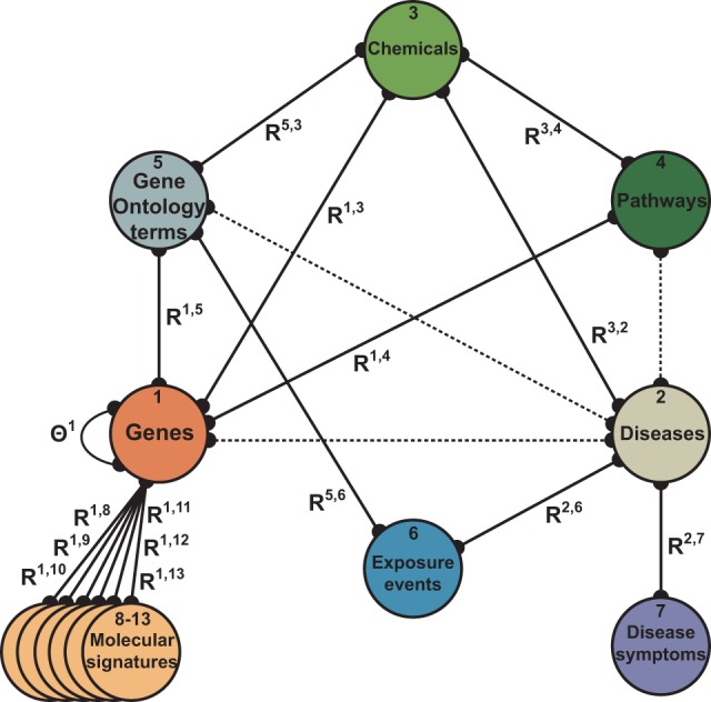
Data fusion graph showing relations between the datasets used in this study. Each node represents a distinct type of objects, such as chemicals, pathways or exposure events, and each edge represents a dataset. For example, $R^{2,6}$ is a matrix of curated exposure data containing environment-disease connections from the CTD database (Davis et al., 2015). In total, the analysis based on this graph considers objects of 13 different types and 16 datasets (ignoring dotted edges, see Section 4.2). For a detailed description of the data, see Section 4.1

Challenges in the joint consideration of systems of datasets, such as that in Figure 1, include inferring accurate models to predict disease traits and outcomes, elucidating important disease genes and generating insight into the genetic underpinnings of complex diseases (Barabási et al., 2011; Han et al., 2013; Ruffalo et al., 2015; Taşan et al., 2015). We would like these models to collectively consider the breadth of available data, from whole-genome sequencing to transcriptomic, methylomic and metabolic data (Navlakha and Kingsford, 2010; Greene et al., 2015; Zitnik et al., 2015). A major barrier preventing existing methods from fully exploiting entire data collections is that individual datasets usually cannot be directly related to each other. For example, datasets $R^{5,3}$ (annotation of chemicals with Gene Ontology (GO) terms) and $R^{2,7}$ (symptoms of diseases) in Figure 1 reside in completely different feature space. As we will learn in this manuscript, we can relate distant objects by chaining through the fusion graph, for example, we can relate molecular signatures with disease symptoms through genes, GO terms, chemicals and diseases. But such chaining actually exacerbates the problem, as distant objects can be linked in many different ways. For example, another way to relate molecular signatures with disease symptoms is via genes, pathways, chemicals, GO terms (Ashburner et al., 2000), exposure events and diseases. A priori, it is not obvious which of the two ways, or which of any existing ways of connecting the signatures with the symptoms, performs better and should thus be preferred when mining disease data.

Different ways of relating objects often carry different semantic meanings and can potentially generate different results. Intuitively, different semantics imply different similarities. However, traditional methods that we review in the next section disregard the subtlety of different types of objects and links. These methods mix, discard or ignore different semantics, which might impede their performance and explanatory capabilities. In this work, we aim to fill this gap by developing an approach for disease module detection that can consider diverse semantics in a principled manner.

We here introduce a novel approach, called Medusa, for automatic detection of size-k significant modules from heterogeneous systems of biological data. Unlike previous works in integrative data analysis, Medusa explicitly takes different semantics into consideration during module detection by allowing a user to either choose a particular semantic or combine them. Our goal is to answer association queries on possibly complex data systems, such as the one in Figure 1. For example, given a small number of diseases, infer the most significant group (module) of genes of size k. Or, given a list of genes, propose a group of k other genes that, taken together, will give the highest significance under a particular null hypothesis. Or, given a selection of molecular pathways of interest, find which k chemicals have the largest collective impact on these pathways. To achieve this level of versatility, Medusa builds upon a recent collective matrix factorization algorithm (Zitnik and Zupan, 2015). In addition, Medusa formulates a submodular optimization program, which provides theoretical guarantees about the significance of the detected modules (Fujishige, 2005).

In a case study with datasets shown in Figure 1, we applied Medusa to find gene–disease associations and infer disease modules. We demonstrate that Medusa-inferred associations are more accurate than those of alternative approaches, which conflate distinct semantics that exist in the data system. Importantly, we find that different semantics vary in their ability to make accurate predictions. We also show that the performance of different semantics depends on the disease category. Finally, we observe that the overall best performance is achieved when Medusa infers associations by combining distinct semantics.

2 Related work

The question of distinguishing different semantics that exist within biomedical data systems remains largely unexplored. Two notable exceptions include a meta-path-based approach for gene–disease link prediction in heterogeneous networks (Himmelstein and Baranzini, 2015) and a latent-chain-based approach for gene prioritization (Zitnik et al., 2015). These approaches, however, are algorithmically different. The approach of Himmelstein and Baranzini (2015) is a network-based technique that relies on meta-paths (Sun et al., 2011a, 2011b, 2012; Wan et al., 2015). Meta-paths represent the number of path instances between two objects that follow a particular sequence of object types in a heterogeneous network. In contrast to meta-paths, Zitnik et al. (2015) use collective matrix factorization (Zitnik and Zupan, 2015) to estimate a latent data representation of a data system and then derive new connections by appropriately multiplying the latent matrices. In Section 5.3, we empirically compare our Medusa, which formulates module detection on top of latent representation of the system, to alternative meta-path-based approaches.

Advances in computational approaches for mining disease related relationships, such as gene–disease, drug–disease or disease–disease associations may lead to better understanding of human disease and may help identify new disease genes, drug targets and biomarkers Barabási et al. (2011). Representative studies include Davis and Chawla (2011); Gonçalves et al. (2012); Köhler et al. (2008); Li and Patra (2010); Warde-Farley et al. (2010); Zitnik et al. (2013). Barabási et al. (2011) and Navlakha and Kingsford (2010) found that random walk approaches usually outperform clustering and neighborhood approaches when predicting gene–disease associations from network data, although most methods make unique predictions not proposed by any other method. Recently, latent factor models (e.g. Natarajan and Dhillon (2014); Zitnik et al. (2013); Zitnik and Zupan (2016)) have been successful in predicting gene–disease and disease–disease associations. These methods can combine heterogeneous data for diseases and genes by estimating latent models that are coupled across different datasets and explain well the observed associations. Cofunction (Ruffalo et al., 2015; Taşan et al., 2015) networks are also important for fine-scale mapping of diseases by prioritizing genes located at disease-associated loci, for example, by connectivity to known causal genes. Most of these approaches are restricted to inferring pairwise associations.

There are several lines of research on how to consider many datasets to derive good groupwise disease associations. Vanunu et al. (2010); Ghiassian et al. (2015) considered network propagation and random walk analysis for prioritizing disease genes and inferring protein complex associations. Han et al. (2013) sought groupwise disease associations for sets of single nucleotide polymorphisms mapping to a given functional category. On a related note, guilty-by-association methods (Wang et al., 2012) have used cofunction networks to assign functions to uncharacterized genes in various organisms and to functionally characterize whole sets of genes. Functionally coherent subnetworks were also used to augment curated functional annotations by connecting genes that share, or are likely to share, functions (Greene et al., 2015; Lee et al., 2004; Taşan et al., 2015), for example, by sharing protein domain annotations or tissue-specific interactions.

However, while these gene–disease association and disease module detection methods use the information from different data sources, none, including our previous work on this topic (Zitnik et al., 2013; Zitnik and Zupan, 2016), explicitly considers that different purposes of disease-related analysis might benefit from considering different, potentially distant, semantics between genes and diseases, nor do they ask users to select/combine different ways of connecting genes with diseases. Medusa, the algorithm presented here, differs from the above methods in that it utilizes semantically distinct chains consisting of possibly many relations to derive relationships between objects, such as genes and diseases. Medusa can establish connections between objects for which direct relationships are not available in present data. It then uses these connections to find size-k modules of objects that together exhibit near-highest significance to the preselected pivot objects. The flexibility of Medusa is further shown in that the object type of the pivots can, but not necessarily, coincide with the object type of the candidates and that chains carrying different semantic meanings can be combined in a principled manner.

3 Methods

Medusa is an approach for the detection of size-k modules that are maximally significant for a predefined set of pivot objects. On the input, Medusa accepts (i) a set of candidate objects that are potential module members, (ii) a set of pivot objects that are not necessarily of the same type as the candidates and (iii) a possibly large and heterogeneous collection of datasets represented in the form of a data fusion graph such as that shown in Figure 1.

Medusa uses collective matrix factorization to jointly estimate a latent data model from all datasets included in a fusion graph. It exploits the latent data model to establish semantically distinct connections between candidate objects and domains of other object types in the fusion graph (Section 3.2). The module detection algorithm in Medusa (Sections 3.3–3.5) is a submodular optimization program which yields an efficient algorithm and provides theoretical guarantees about the significance of the detected modules.

3.1. Preliminaries and notation

3.1.1. Data fusion graph

A data fusion graph $\mathcal{G}=(\mathcal{V},\mathcal{R},\mathcal{T})$ is a relational map of datasets (Zitnik and Zupan, 2015). Nodes of the graph $\mathcal{V}$ represent different types of objects, such as ontological terms, genes, diseases, pathways and chemicals. The edges of the graph correspond to datasets, which are given in matrices annotated next to the edges. An exemplar data fusion graph is shown in Figure 1. Matrix $R^{2,7}$ therein is a $n_2\times n_7$ real-valued matrix whose rows correspond to diseases indexed by a respective disease-based controlled vocabulary and whose columns indicate disease symptoms indexed by a symptom-based vocabulary. Elements of matrix $R^{2,7}$ represent a dataset, such as disease–symptom associations.

Technically, the edges of the fusion graph are given by a set of relation matrices $\mathcal{R}=\{R^{I,J};I,J\in \mathcal{V},I\ne J,R^{I,J}\in {ℝ}^{n_I\times n_J}\}$ that represent dyadic datasets and a set of constraint matrices $\mathcal{T}=\{{\Theta }^I;I\in \mathcal{V},{\Theta }^I\in {ℝ}^{n_I\times n_I}\}$ that represent unary datasets. It is possible to have multiple relation matrices that relate object types I and J (i.e. more than one edge between I and J in the fusion graph) or multiple constraint matrices for object type I (i.e. more than one loop for I in the fusion graph). Here, this possibility is suppressed for notational brevity.

3.1.2 Collective matrix factorization

Collective matrix factorization (Zitnik and Zupan, 2015) is an algorithm that considers a fusion graph $\mathcal{G}=(\mathcal{V},\mathcal{R},\mathcal{T})$ and infers its latent model by compressing the datasets with co-factorization of matrices in $\mathcal{R}$. Matrices $\mathcal{T}$ are used for regularization of the latent model. The method simultaneously co-factorizes all the relation matrices into the products of much smaller latent matrices through a procedure which (i) ensures the transfer of information between related matrices and (ii) promotes good generalization via a high-quality data compression. To achieve the first point, collective factorization reuses the latent matrices when decomposing distinct but related relation matrices. The second feature is possible due to the low-dimensional nature of matrix factorization.

The collective matrix factorization algorithm aims to estimate low-dimensional latent matrices $G^I,I\in \mathcal{V}$, and $S^{I,J},I,J\in \mathcal{V}$, which minimize the following objective:

$${\displaystyle \sum _{R^{I,J}\in \hspace{0.5em}\mathcal{R}}}\left|\right|R^{I,J}-G^I{S}^{I,J}{(G^J)}^T|{|}_{\text{Fro}}^2+{\displaystyle \sum _{{\Theta }^I\in \hspace{0.5em}\mathcal{T}}}\text{\hspace{0.17em}tr}({(G^I)}^T{\Theta }^I{G}^I).$$ (1)

Here, the inferred latent matrices tri-factorize each relation matrix as ${\widehat{R}}^{I,J}=G^I{S}^{I,J}{(G^I)}^T$. Matrix $G^i$ is a $n_I\times k_I$ ($k_I\ll n_I$) non-negative latent matrix containing latent profiles of objects of type I in rows, G^J is a $n_J\times k_J$ ($k_J\ll n_J$) non-negative latent matrix with profiles of objects of type J in rows and $S^{I,J}$ is a $k_I\times k_J$ latent matrix that models interactions between latent components in the (I, J)-th dataset. The latent profile of an object of type I is given by its corresponding row vector in $G^I.$ Semantically, the profile encodes membership of the object to the k_I latent components.

The parameters of the algorithm are factorization ranks, k_I, for every object type I in the data fusion system, which are selected as in Zitnik et al. (2015). We refer the reader to Zitnik and Zupan (2015) for a detailed description and theoretical analysis of the factorization algorithm.

3.1.3. Chaining of latent data matrices

A factorized system of latent data matrices returned by the collective matrix factorization can be used to establish connections between distant object types, i.e. non-neighboring nodes in the fusion graph (Zitnik et al., 2015).

Definition 1 —

Chain: A chain ${\mathcal{C}}^{S,T}$ is a sequence of relations defined on a fusion graph $\mathcal{G}=(\mathcal{V},\mathcal{R},\mathcal{T})$ that connects object type $S\in \mathcal{V}$ with possibly distant object types $T\in \mathcal{V}.$ The chain ${\mathcal{C}}^{S,T}$ is denoted in the form of:

$${\mathcal{C}}^{S,T}=R^{S,I_1}○R^{I_1,I_2}○\dots ○R^{I_{l-2},I_{l-1}}○R^{I_{l-1},T},$$ (2)

which defines a composite relation between object types S and T, where $○$ denotes the composition operator on relations. Here, for $I_1,I_2,\dots ,I_l$ the object types I_j and $I_{j+1}$ must be adjacent in the fusion graph $\mathcal{G}$.

The length l of chain ${\mathcal{C}}^{S,T}$ is measured by the number of its constituent relations. We now formulate how to materialize a given chain and derive the profiles of objects of one type in the space of objects of another type.

Definition 2 —

Materialized chain: Given a fusion graph $\mathcal{G}=(\mathcal{V},\mathcal{R},\mathcal{T})$ and a latent data system estimated by collective matrix factorization, a materialized chain $C^{S,T}\in {ℝ}^{n_S\times n_T}$ for chain ${\mathcal{C}}^{S,T}$ specified in Equation (2) is defined as:

$$C^{S,T}={\widehat{R}}^{S,I_1}{\widehat{R}}^{I_1,I_2}\dots {\widehat{R}}^{I_{l-2},I_{l-1}}{\widehat{R}}^{I_{l-1},T},$$ (3)

where ${\widehat{R}}^{I,J}$ is the relation matrix reconstructed from the latent data system as ${\widehat{R}}^{I,J}=G^I{S}^{I,J}{(G^J)}^T.$ (${(·)}^T$ is matrix transposition.)

3.1.4. Submodular functions and optimization

Submodular functions (Edmonds, 1970; Fujishige, 2005) have recently attracted much interest, e.g. see Krause and Guestrin (2011). Let us assume we are given a finite set of n objects V and a valuation function $f:2^V\to {ℝ}_{+}$ that returns a non-negative real value for any subset $X\subseteq V.$ The function f is said to be submodular if it satisfies the property of diminishing returns. That is, for any set $X\subseteq Y$ and $i\cancel{\notin }Y$, we must have: $f(X\cup \{i\})-f(X)\ge f(Y\cup \{i\})-f(Y).$ This means that the incremental gain of element i decreases when the background in which i is considered grows from X to $Y\supseteq X.$ We define the ‘gain’ as $f(i,X)=f(X\cup \{i\})-f(X)$, which implies that f is submodular if $f(i,X)\ge f(i,Y).$

In this article, we deal with functions that are not only submodular but also non-negative (i.e. $f(X)\ge 0$ for all $X\subseteq V$) and monotone non-decreasing (i.e. $f(X)\ge f(Y)$ for all $X\subseteq Y$). Such functions are trivial to uselessly maximize, since f(V) is the largest possible valuation. However, we would typically like to identify a valuable subset of bounded and small cost. Here, we are interested in subsets whose costs are measured by their size. This leads to the optimization problem $X^{*}\in \text{arg\hspace{0.17em}}{\text{max}}_{X\subseteq V,\left|X\right|\le k}f(X),$ where k is the desired subset size. Solving this problem exactly is NP-complete (Feige, 1998). However, when f is submodular, then the greedy algorithm has a worst case guarantee of $f({\tilde{X}}^{*})\ge (1-1/e)f(X_{\text{opt}})\approx 0.63f(X_{\text{opt}})$, where $X_{\text{opt}}$ is the optimal and ${\tilde{X}}^{*}$ is the greedy solution (Nemhauser et al., 1978).

3.2. Problem definition

In this section, we introduce a framework for module detection on data fusion graphs, a novel approach to find size-k maximally significant modules, Medusa, and propose a Medusa-based top-k module detection problem that takes into consideration diverse semantics in heterogeneous data systems.

We start by defining the concepts needed to guide the module detection procedure and to assess the significance of the modules.

Definition 3 —

Candidate objects: Given a fusion graph $\mathcal{G}=(\mathcal{V},\mathcal{R},\mathcal{T})$, candidate objects are given by a set $I=\{i_1,i_2,\dots ,i_{n_I}\}$ of all the entities that belong to type $I\in \mathcal{V}.$ Candidates constitute a pool of objects from which a module is identified.

Definition 4 —

Pivot objects: Given a fusion graph $\mathcal{G}=(\mathcal{V},\mathcal{R},\mathcal{T})$, pivot objects are given by a subset $S_0=\{s_1,s_2,\dots ,s_u\},$$u<n_J$, of the entities of type $J\in \mathcal{V}.$ Pivots are the objects against which the significance of the current Medusa module is assessed.

Depending on whether the pivots and the candidates belong to the same or different type of objects in $\mathcal{G}$, we distinguish two prediction settings. This distinction is important because it will lead to different optimization objectives when detecting modules in Section 3.4.

Task 3.1 —

We aim to find a size-k module $M_k=\{m_1,m_2,\dots ,m_k\}$ of the candidates I that display the maximal significance with respect to the given pivots S₀.

Let J be the object type of the pivots. (i) In the candidate-pivot-equivalence (CPE) regime, candidates and pivots are of the same data type, $I=J.$ (ii) In the candidate-pivot-inequivalence (CPI) regime, candidates and pivots are of different types, $I\ne J.$

We illustrate the CPE and the CPI regimes with concrete examples in Figures 2 and 3, respectively. We proceed by formulating a measure, which we optimize for when detecting Medusa modules.

Fig. 2.

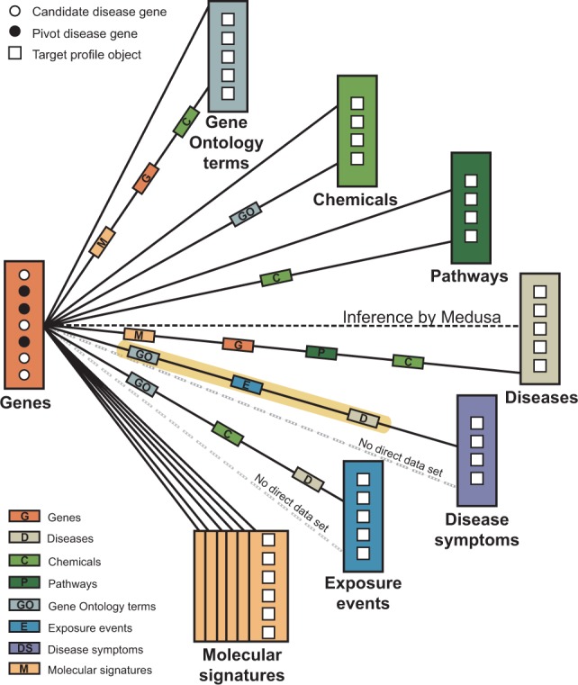
The CPE regime in Medusa. In the CPE environment, Medusa detects a relevant module of candidate objects based on a set of pivot objects, which belong to the same object type as the candidates. For example, given three disease genes (pivots, black circles), we want to find other potentially relevant disease genes (candidates, white circles), a task denoted with a black dashed line. In a special case where the studied objects are genes, as shown here, and we are interested in size-1 modules, the CPE regime coincides with the well-known gene prioritization task. The figure shows 15 distinct semantic aspects (solid black lines) that exist in the fusion graph in Figure 1 to relate genes with all other types of objects. For example, one semantic to relate genes with disease symptoms goes through Gene Ontology terms (‘GO’), exposure events (‘E’) and diseases (‘D’). Notice that we cannot directly relate genes to disease symptoms, i.e. at least one other object type is needed to establish the connection (gray dashed line)

Fig. 3.

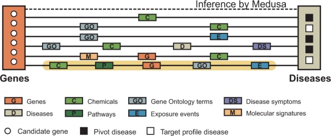
The CPI regime in Medusa. In the CPI regime, Medusa detects a relevant module of candidate objects based on a set of pivot objects, which belong to a different object type than the candidates. For example, given three diseases (pivots, black squares), we want to find potentially relevant genes (candidates, white circles), a task denoted with a dashed line. The figure shows six distinct semantics (solid lines) that exist in the fusion graph in Figure 1, which Medusa can choose or combine to identify the relevant module. For example, highlighted is an aspect that connects genes with diseases via chemicals (‘C’), pathways (‘P’), genes (‘G’), Gene Ontology terms (‘GO’) and exposure events (‘E’)

3.3. Submodularity for detection of Medusa modules

Submodularity is a natural model for detection of size-k maximally significant modules in multiplex data. In this case, each $i\in V_{\text{source}}$ is a distinct candidate and $V_{\text{source}}$ corresponds to a set of all candidate objects. An important characteristic of a good model for this problem is that we wish to decrease the ‘value’ of a candidate $i\in V_{\text{source}}$ based on how much that candidate has in common with candidates S_r that have been chosen in the first r rounds.

The value $p(i,S_r)$ of a given candidate i in a background of previously chosen objects $S_r\subseteq V_{\text{source}}$ further diminishes as the background grows $V_{\text{source}}\supseteq S_t,t>r.$ When, for example, both candidate and pivot objects are genes and a candidate’s value is represented as the statistical significance of its concentration, it is natural for the significance to be discounted based on how much representation of that candidate already exists in a previously chosen subset. When the module grows, it naturally becomes more diverse, and hence, its characterization is less distinctive, which results in the overall reduction of statistical power. This means that the candidate is pulled into the module when its significance towards the pivot objects is the highest. If the candidate were added to the module later, its significance could only be smaller. That is, if we were to observe that candidate after being included into the module, its significance would fade into insignificance.

This paradigm corresponds to submodularity, which we express mathematically by functions in Equations (5) and (7) below.

3.4. Detection of size-k maximally significant modules

Next, we describe the Medusa module detection algorithm. Recall that Medusa is able to operate in two prediction regimes defined in Section 3.2. We start by describing the algorithm for the CPE regime and proceed with the algorithm for the CPI regime.

Recall that a particular semantic aspect connecting object types S and T is realized as matrix $C^{S,T}$ (Definition 2). For notational convenience, we here denote a given aspect simply as a matrix $C.$ Prior to the analysis, matrix C is row-wise normalized by the sum of the matrix rows, and then multiplied by the number of matrix columns.

3.4.1. Medusa in the CPE regime

We capture the distinct connectivity patterns of the candidates by evaluating the significance of their connections in matrix $C.$ For a randomly picked candidate we evaluate the probability that a certain fraction of the candidate’s strongest connections to the objects in the columns of matrix C match exactly with the strongest connections of the pivots.

In the simplest case, we would simply count the connections, and this notion would correspond to the hypergeometric distribution. However, since matrix C is a real-valued object inferred by a latent model, we take into account the estimated strength of connectivity rather than its mere existence (cf. experiments in Section 5.3). For this, we need to extend the binomial coefficient to the real line using the gamma function (Fowler, 1996). Technically, this is implemented in the following definition.

Definition 5 —

Candidate concentration: Given a semantic $C,$ pivots S₀, and a candidate i, we define the concentration of candidate i as:

$$\begin{array}{l}{h}_{\text{CPE}}(c,S_0,Q_i)=\text{Bin}({\displaystyle \sum _{q\in Q_i}{C}_{S_{0}q}^T}{w}_{S_0},c)\times \\ \text{Bin}({\displaystyle \sum _j{C}_{S_{0}j}^T}\delta (w_{S_0})-{\displaystyle \sum _{q\in Q_i}}{C}_{S_{0}q}^T{w}_{S_0},C_{i}1-c)\times \\ 1/\text{Bin}({\displaystyle \sum _j{C}_{S_{0}j}^T}\delta (w_{S_0}),C_{i}1),\end{array}$$ (4)

where c is the observed strength of connectivity of candidate i, $\text{Bin}(n,k)=\Gamma (n+1)/(\Gamma (k+1)\Gamma (n-k+1)),$ and $\Gamma (x)$ is the gamma function evaluated at x. Here, $\delta (x)$ is the indicator function, $\delta (x)=1$ if x = 1 and $\delta (x)=0$ otherwise. Also, $X_{S_0}$ returns the rows of X indexed by set $S_0.$ Here, Q_i is a set containing column indices of i’s strongest connections. The weights in vector w are defined as $w_i=1$ if $i\in S_0$, else $w_i={(1-\alpha )}^r$ if $i\in S_r,$ where r is the iteration when i was included into the module, and $w_i=0$ otherwise. The value for $\alpha ,$ which promotes modules that are tight around the initial set of pivots S₀, and the size of Q_i, are user-defined parameters.

We evaluate whether candidate i has greater correspondence with the pivots than expected under this null hypothesis by calculating the cumulative probability for the observed or any weaker concentration of the connectivity:

$$p_{\text{CPE}}(i,S_0;Q_i)\triangleq {{\displaystyle \int }}_{\left|Q_i\right|}^{{\tilde{c}}_i}{h}_{\text{CPE}}(c,S_0,Q_i)dc$$ (5)

where ${\tilde{c}}_i=C_{i{Q}_i}1.$ A better candidate will have a lower $p_{\text{CPE}}$ value.

It can be shown that the use of this cumulative probability to select a candidate object, which is to be included into the current module, leads to a submodular program (the proof is omitted here for brevity). This appealing property allows us to use the greedy algorithm to find modules of size k that approximate the optimal modules within a constant factor (Section 3.1.4). Recall that the optimal modules can only be found using a prohibitively expensive exhaustive enumeration of all size-k modules. Building on these observations, we propose the algorithm to identify a maximally significant module of size k, which solves Task 3.1 in the CPE regime:

1. Start with an empty module $M_0=\left\{\right\}$.

2. Compute concentration significance (Equation (5)) for all candidates.

3. Rank the candidates according to their respective $p_{\text{CPE}}$ values.

4. Add the candidate i with the highest rank (i.e. lowest $p_{\text{CPE}}$ value) to the current Medusa module, $M_r\to M_{r+1}=M_r\cup \left\{i\right\}$, and to the set of pivot objects, $S_r\to S_{r+1}=S_r\cup \left\{i\right\}.$

5. Repeat steps 2–4 k-times with the expanded set of pivot objects.

The order in which the candidates are pulled into the module reflects their relevance to the pivot objects according to semantic $C.$ Figure 4 is an example for finding a size-3 gene module based on a semantic that relates genes to disease symptoms via GO terms, exposure events and diseases.

Fig. 4.

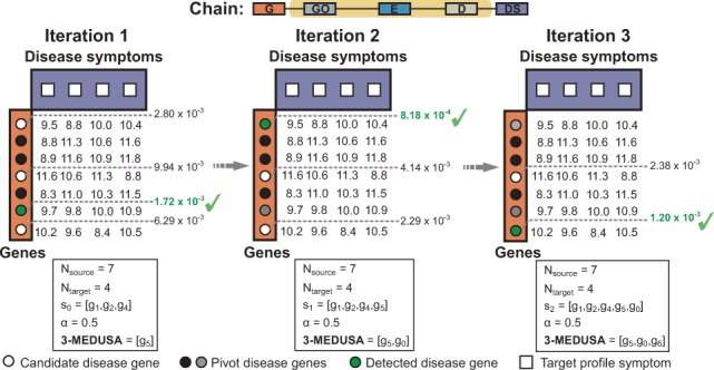
Inferring a three-maximally significant distant module with Medusa in the CPE regime. Shown is a toy example of a chain that relates seven genes in rows to four disease symptoms in columns via GO terms, exposure data and diseases (see the highlighted chain in Fig. 2). Given the three pivot genes shown as black circles, we would like to identify the most significant size-3 gene module. Notice that we operate in the CPE regime where both pivot and candidate objects are of the same type (i.e. genes). In the first iteration, candidate g₅ achieves the lowest score (i.e. $p_{\text{CPE}}=1.72\times {10}^{-3}$) and is thus added to the module and included into the pivot set. However, the importance of g₅ as a pivot object is downweighted according to the $\alpha =0.5$. Notice also that candidate g₃ has a predominantly reversed concentration relative to the pivot genes $g_1,g_2,g_4$ in the first iteration, which results in the poor score of g₃ (i.e. $p_{\text{CPE}}=9.94\times {10}^{-3}$). In particular, candidate g₃ is concentrated on symptoms d₀ and d₂, whereas pivot genes are concentrated on d₁ and d₃. The score for g₃ improves in later iterations when the Medusa module becomes more diverse. The final module is $M_3=\{g_5,g_0,g_6\}.$

3.4.2. Medusa in the CPI regime

So far, we have seen that in the CPE regime, candidates and pivots are given by the rows of matrix C. However, in the CPI regime this is not true anymore. Here, pivots correspond to columns of matrix $C,$ whereas candidates are still given by rows of matrix $C.$ To adjust for this change, we assess a candidate’s significance by its visibility, which we define next.

Definition 6 —

Candidate visibility: Given a semantic $C,$ pivots S₀ and a candidate i, we define the visibility of candidate i as:

$$\begin{array}{l}{h}_{\text{CPI}}(c,S_0)=\text{Bin}({\displaystyle \sum _j{C}_{j{S}_0}}1,c)\times \\ \text{\hspace{0.17em}\hspace{0.17em}\hspace{0.17em}\hspace{0.17em}\hspace{0.17em}\hspace{0.17em}\hspace{0.17em}\hspace{0.17em}\hspace{0.17em}\hspace{0.17em}\hspace{0.17em}\hspace{0.17em}\hspace{0.17em}\hspace{0.17em}\hspace{0.17em}\hspace{0.17em}\hspace{0.17em}\hspace{0.17em}\hspace{0.17em}\hspace{0.17em}\hspace{0.17em}\hspace{0.17em}\hspace{0.17em}\hspace{0.17em}Bin}({\displaystyle \sum _{l,j}{C}_{lj}}-{\displaystyle \sum _j{C}_{j{S}_0}}1,C_{i}1-c)\times \\ 1/\text{Bin}({\displaystyle \sum _{l,j}{C}_{lj}},C_{i}1).\end{array}$$ (6)

The notation follows that in Equation (4).

Intuitively, the visibility of a candidate is the strength of its connections with the pivots. We evaluate whether candidate i has stronger connections to the pivots than expected under this null hypothesis by calculating the cumulative probability for observed or any stronger visibility:

$$p_{\text{CPI}}(i,S_0)\triangleq {{\displaystyle \int }}_{{\tilde{c}}_i}^m{h}_{\text{CPI}}(c,S_0)dc$$ (7)

where ${\tilde{c}}_i=C_{i{Q}_i}1$ and m is the number of columns in $C.$ A better candidate will have a lower $p_{\text{CPI}}$ value.

Similarly as for the CPE regime, the use of cumulative probability $p_{\text{CPI}}$ leads to a submodular optimization program, which has the same appealing properties as the cumulative probability $p_{\text{CPE}}$ in Section 3.4.1. Building on the theory of submodular functions, we tackle Task 3.1 in the CPI regime by proposing the following greedy algorithm to identify a maximally significant module of size k:

1. Start with an empty module $M_0=\left\{\right\}$.

2. Compute visibility significance (Equation (7)) for all candidates. Visibility of candidate i naturally decreases in iteration r according to ${\tilde{c}}_i=(1-{\sum }_{t=1}^r{\beta }^t\exp (-\text{KL}(C_i,C_{x_{t-1}})))C_{i{S}_0}1,$ where KL denotes the Kullback–Leibler divergence, $C_{x_{t-1}}$ is matrix row of the candidate selected in iteration t − 1 and β is a user-defined parameter promoting diverse modules.

3. Rank the candidates according to their respective $p_{\text{CPI}}$ values.

4. Add the candidate i with the highest rank (i.e. lowest $p_{\text{CPI}}$ value) to the current Medusa module, $M_r\to M_{r+1}=M_r\cup \left\{i\right\}$.

5. Repeat steps 2–4 k-times, bringing in one candidate object at a time into the growing module.

Figure 5 shows a toy example for finding a size-3 gene module based on a semantic that relates genes with diseases via chemicals, pathways, genes, GO terms and exposure events.

Fig. 5.

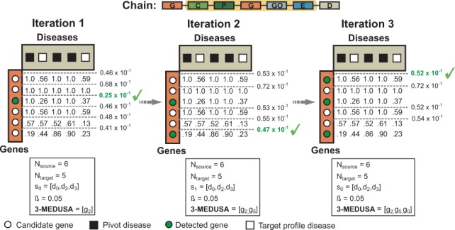
Inferring a three-maximally significant distant module with Medusa in the CPI regime. Shown is an example of a chain that relates six genes to five diseases via chemicals, pathways, genes, GO terms and exposure data (see the highlighted chain in Fig. 3). In this toy example, we are given three pivot diseases shown in black squares and would like to find a three-maximally significant gene module. Notice that we operate in the CPI data regime because the pivots (i.e. diseases) are of different type than the candidates (i.e. genes). In the first iteration, gene g₂ shows the most significant visibility for the pivot diseases (i.e. $p_{\text{CPI}}=0.25\times {10}^{-1}$) and is thus included into the module. Gene g₁ does not discriminate between the pivot and non-pivot diseases and is hence considered an unlikely candidate (i.e. $p_{\text{CPI}}=0.68\times {10}^{-1}$ in the first iteration and $p_{\text{CPI}}=0.72\times {10}^{-1}$ in later iterations). In second iteration, the algorithm picks g₅, although one might expect that g₁ would be selected due to its distinctive connections to the pivot disease. This is because Medusa detects modules that are not only highly visible to the pivot objects but are also diverse, which is important when trying to identify non-redundant comprehensive modules. Such behavior of Medusa is regulated by parameter β, which promotes diverse modules in this example, $\beta =0.05$. The final module is $M_3=\{g_2,g_5,g_0\}$

3.5. Combining chains carrying different semantics

So far, we have described the Medusa algorithm that operates on one particular semantic given by a single matrix C. To be able to combine d different semantics, given by a set of chained matrices $C^{(1)},C^{(2)},\dots ,C^{(d)}$, we employ the following technique.

In the r-th iteration of Medusa, we independently score the candidates according to Equation (5) (in the case of the CPE regime) or Equation (7) (in the case of the CPI regime) for all matrices $C^{(1)},C^{(2)},\dots ,C^{(d)}.$ We then combine candidate scores from different semantics into one score per candidate by an affine combination of semantics’ weights.

In the CPE regime, this is done such that the semantics which rank the pivots higher are assigned larger weights than those in which the pivots are ranked lower. Intuitively, this means that semantics that are more informative for the given set of pivots contribute more towards the final candidate score.

In the CPI regime, the combination of semantics is done such that the semantics in which the pivots have more similar profiles measured by the KL divergence are assigned larger weights than those in which the pivots have more heterogeneous data profiles. Detailed steps are provided within the online implementation of Medusa.

Once the aggregated candidate scores are calculated, Medusa uses algorithms from Sections 3.4.1 and 3.4.2 to detect the modules.

4 Experimental setup

4.1. Datasets in the data fusion graph

In our experiments, we consider a collection of datasets shown in Figure 1. Table 1 lists public sources from which data were obtained to build 16 data matrices.

Table 1.

Datasets used for the analyses presented in this article

Matrix	Reference	Size	Matrix	Reference	Size
$R^{1,5}$	Ashburner (2000)	$19828\times 19951$	$R^{5,6}$	Davis (2015)	$19951\times 565$
$R^{1,3}$	Davis (2015)	$19828\times 12614$	$R^{1,8}$	Subramanian (2005)	$19828\times 326$
$R^{1,4}$	Davis (2015)	$19828\times 291$	$R^{1,9}$	Subramanian (2005)	$19828\times 3,395$
$R^{2,6}$	Davis (2015)	$9350\times 565$	$R^{1,10}$	Subramanian (2005)	$19828\times 186$
$R^{2,7}$	Zhou (2014)	$9350\times 321$	$R^{1,11}$	Subramanian (2005)	$19828\times 1,330$
$R^{3,2}$	Davis (2015)	$12614\times 9350$	$R^{1,12}$	Subramanian (2005)	$19828\times 221$
$R^{3,4}$	Davis (2015)	$12614\times 291$	$R^{1,13}$	Subramanian (2005)	$19828\times 615$
$R^{5,3}$	Davis (2015)	$19951\times 12614$	${\Theta }^1$	Chatr-Aryamontri (2014)	$19828\times 19828$

GO (Ashburner et al., 2000) annotations were downloaded from http://geneontology.org in December 2015 containing 481 685 human gene product annotations. UniProt protein accession identifiers were collapsed to human NCBI’s Entrez gene identifiers using the mapping provided by the HUGO Gene Nomenclature Committee resource (Gray et al., 2015). Curated human protein–protein interactions were retrieved from the BioGRID 3.4.131 database (Chatr-Aryamontri et al., 2014). The recourse contained interactions for 19 702 genes. Data on clinical manifestation of diseases were obtained from the human symptoms–disease network (HSDN; Zhou et al., 2014; Suppl. data S4) and included 147 978 relationships between symptoms and diseases. Term co-occurrences between symptoms (MeSH Symptom terms) and diseases (MeSH Disease terms) were weighted by the TF-IDF values.

We also compiled gene sets from the Molecular Signatures Database (MSigDB; Subramanian et al., 2005) in December 2015: 326 positional gene sets (MSig-C1) corresponding to each human chromosome and each cytogenetic bands; 3395 curated gene sets (MSig-C2) representing expression signatures of genetic and molecular perturbations; 1330 gene sets (MSig-C2) corresponding to canonical representations of biological processes from the pathway databases; 186 gene sets (MSig-C2) derived from the KEGG database; 221 motif gene sets (MSig-C3) with genes sharing microRNA binding motifs; and 615 gene sets (MSig-C3) with genes sharing transcription factor binding sites. Curated chemical–gene interactions ($R^{1,3}$), chemical–pathway interactions ($R^{3,4}$), gene–pathway associations ($R^{1,4}$), chemical–function associations ($R^{5,3}$), chemical–disease ($R^{3,2}$), function–exposure events ($R^{5,6}$), exposure event–disease relationships ($R^{2,6}$) and gene–disease relationships were retrieved from the Comparative Toxicogenomics Database (CTD; Davis et al., 2015) in December 2015.

Each dataset was represented with a real-valued data matrix as indicated in Table 1. Prior to the analysis, all matrices were independently column–row normalized according to the second vector norm.

4.2. Disease modules and gene–disease associations

The corpus of 310 diseases was downloaded from the CTD (Davis et al., 2015) with the criteria that every disease should have at least 10 and at most 100 curated gene associations for which direct evidence is available in the CTD database. These diseases and their associated genes constituted our ground-truth information against which we evaluated disease module detection and gene–disease association prediction. On average, each disease had 28 associated genes.

To ensure there was no leakage of information from training to test set in our integrative analysis, we used the following protocol. From our data system we excluded datasets that directly or indirectly rely on disease–gene associations (dotted lines in Fig. 1). For example, we skipped the pathway-to-disease dataset (a hypothetical data matrix $R^{4,2}$ in Fig. 1) because a particular pathway would only be linked to a particular disease if there was a disease-associated gene in this pathway. Another example of an excluded dataset is the GO term-to-disease dataset (a hypothetical data matrix $R^{5,2}$ in Fig. 1). Here, a given term and a given disease would be linked only if there existed a gene that was both annotated with the term in the GO and associated with the disease.

This protocol enabled us to construct a data system for performance evaluation of various methods that was not contaminated by existing gene–disease associations. For example, dataset $R^{3,2}$ in Figure 1 contained curated chemical–disease associations that were extracted from the published literature by the CTD curators (Davis et al., 2015). However, this dataset omitted inferred chemical–disease associations from our training data, which associated chemicals and diseases through shared gene interactions.

4.3. Performance evaluation

We evaluated prediction accuracy using a disease-centric cross-validation procedure. (i) Prediction of gene–disease associations was evaluated as follows. For a particular disease in our corpus of 310 diseases, we conducted a leave-one-gene-out cross-validation to obtain an estimated score for the left-out gene. The remaining (training) genes were considered positive instances and were used to select and fit the model parameters. (ii) Detection of disease modules was evaluated using the procedure from Ghiassian et al. (2015). For each disease module, we randomly removed a certain fraction (25%, 50% and 75%) of the disease genes and used the remaining genes as pivots.

For Medusa, we need to specify the parameters required by collective matrix factorization, the value for α, the size of Q (in the case of the CPE regime) and the value for β (in the case of the CPI regime). We tuned α, β and the size of Q in an internal cross-validation procedure on the training genes. Factorization ranks for collective matrix factorization were selected using a procedure similar to the one described in Zitnik et al. (2015); 13 values were required, each representing latent dimension of one object type in our fusion graph. We selected these dimensions through a single parameter p, which specified latent dimension for an object type as a fraction of the number of objects of that type: $k_I=p{n}_I.$ The value p = 0.05 was used in the experiments because it maximized the mean areas under precision-recall curves (AUPRC) achieved on a set of 10 diseases from the CTD, which were later not considered for performance comparison. The selection of parameters for other approaches was made based on internal cross-validation.

We measured accuracy using the AUPRC and the area under the receiver operating characteristic curve (AUROC).

5 Results and discussion

5.1. Capturing biological semantics with Medusa

First, our goal was to investigate the effects of different biological semantic aspects on the prediction of gene–disease associations. We used Medusa to estimate disease genes for 310 diseases included in the CTD database (Section 4.1). We considered eight distinct semantic aspects denoted as C1–C8 (Fig. 6, left). For example, chain C6 corresponds to a matrix that relates genes to diseases via GO terms and exposure events (see Definition 2).

Fig. 6.

Gene–disease association prediction with Medusa. Nine different biological semantics (C1–C8, CA) were considered in the analysis. Each semantic is shown as a sequence of object types contained in the fusion graph (Fig. 1). For example, in the ‘C4’ semantic, Medusa estimated gene–disease associations based on the latent chain that related genes (‘G’) with disease symptoms (‘DS’) via Gene Ontology terms (‘GO’), chemicals (‘C’), diseases (‘D’) and disease symptoms (‘DS’). For each distinct biological semantic we report the AUROC and AUPRC values aggregated over 310 complex diseases. For visualization purposes, diseases were partitioned into 25 disease classes based on Disease Ontology (Kibbe et al., 2014), such as ‘reproductive system diseases’ and ‘musculoskeletal system diseases’, and the points representing accuracy scores of each individual disease are colored according to corresponding disease classes. Notice the substantial variation of performance across different semantics. Generally, Medusa achieved the highest accuracy when combining semantics from C1–C8 (i.e. CA, last row).

Medusa detects significant modules of a specified size k. To apply it to the prediction of gene–disease associations, we search for size-1 modules and use probability estimates returned by the algorithm (Equation (5)) to make predictions.

Figure 6 shows the performance of Medusa in terms of AUROC and AUPRC. In addition to the eight distinct semantics, we also analyzed the performance of Medusa in its mode, which combines different semantic aspects, denoted as CA in the figure (Section 3.5). We further studied how prediction accuracy varies across classes of diseases, which were identified using Disease Ontology (Kibbe et al., 2014). A cutoff at level 2 of the Disease Ontology graph revealed 25 disease classes (Fig. 6), such as ‘cognitive disorders’ and ‘gastrointestinal diseases’.

We observed substantial variation of AUROC and AUPRC values across different semantic aspects (i.e. chains). In terms of the AUROC, the best single semantic appeared to be C1, which was followed closely by C3 and C5. In addition to genes, chemicals were the common object type considered for construction of these three chains. These results are important because they demonstrate that different ways of establishing connections between genes and diseases can result in more or less accurate predictions. The results also suggest that objects of different types and links carry different semantic meanings, and it might not make sense to mix them without distinguishing their semantics when associating genes with diseases. This experiment also alludes to the explanatory value of Medusa. Medusa is able to provide insights into the utility of different semantics, a capability, which most present models for co-factorization of multiple matrices do not have.

While a user might explicitly specify a semantic that he would like to consider in a concrete application, Medusa can also make predictions that are consistent with multiple chains. In particular, combining semantics C1–C8 in Figure 6 yielded the most accurate predictions overall. However, prediction accuracy in Figure 6 varies greatly by disease and we explore this issue next.

5.2. Detecting disease modules with Medusa

We analyzed the extent to which Medusa could recover the full disease module if we removed a certain fraction of disease associated genes. Recall that a disease module is given by the set of genes associated with that disease in the CTD (Davis et al., 2015). For a given disease, Medusa used 50% of the disease genes as pivots and detected a size-k module, where k was set to the size of the full disease module. Notice that Medusa pulls in one gene at a time into the growing module and given the inferred latent model, the running time of the module detection increases linearly with the desired module size k. Figure 7 shows the fraction of held-out disease genes (recall) that were found in Medusa modules. Higher values indicate better performance.

Fig. 7.

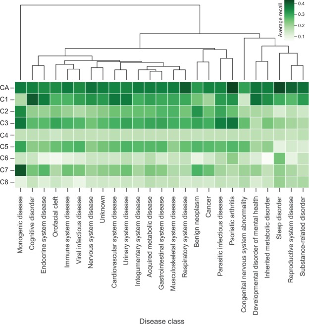
Disease module detection with Medusa. We considered nine different semantic meanings (C1–C8, CA; rows in the heat map) listed in Figure 6. Reported is the recovery rate when 50% of genes from known disease modules were left out. The recall values were calculated for 310 diseases in our corpus and then average aggregated into 25 groups based on a categorization of diseases in the Disease Ontology (Kibbe et al., 2014; columns in the heat map). The dendrogram reveals that recovery rates of disease modules from related disease classes are similar.

We found that the highest rate of true positives was achieved in the early iterations of the Medusa algorithm, i.e. when the number of executed iterations was less than the size of the full module. This is an important observation because it indicates that the highest ranked genes are most likely to be part of the disease module.

The results in Figure 7 further show that the estimated recovery rates varied across different semantic aspects as can be seen by comparing rows in the heat map. Typically, the best performance was observed when Medusa was used to detect modules based on joint analysis of all semantics (see CA in Fig. 7).

It is interesting to examine which classes of diseases display higher recovery rates than others and how the rates compare to each other. The dendrogram in Figure 7 shows that ‘monogenic diseases’ exhibited a distinct recovery pattern. For example, modules corresponding to monogenic disorders according to Disease Ontology (Kibbe et al., 2014) were best recovered using the chain C7, whereas other disease classes (with the exception of cognitive disorders) were best detected when Medusa was used in the CA setting. We also observed that related disease classes displayed similar patterns of recovery rates across different semantics. For example, immune system diseases and viral infectious diseases are placed closely together in the dendrogram, as well as acquired metabolic diseases and diseases of the gastrointestinal system. It is known that diseases from similar disease classes are more likely to be associated with sets of genes that overlap (Barabási et al., 2011). The similar recall patterns from related disease classes thus suggest that the Medusa outcome is robust with respect to variations in the set of pivot genes.

5.3. Comparing Medusa with existing methods

So far we have studied the utility of Medusa to take into consideration distinct semantics that exist in heterogeneous biological data when predicting gene–disease associations and detecting disease modules. We proceed by examining how Medusa performs relative to several other approaches for mining gene–disease associations.

First, we compare Medusa with meta-path based approaches (Section 2). These approaches have just recently been tested on prediction problems in biology for the first time (Himmelstein and Baranzini, 2015) and have shown promising performance for prioritizing genetic associations from genome-wide association studies. Meta-paths (Sun et al., 2011b) are sequences of object types. They are used to represent complex relationships between objects beyond what links in a homogeneous network capture. For example, given a meta-path that corresponds to the chain C6: Genes → GO terms → Exposure events → Diseases (Fig. 6, left), a meta-path-based approach in its simplest form relates a particular candidate gene with a particular pivot disease by counting the number of paths in a heterogeneous network between a candidate and pivot node. These counts then serve to derive features. Each feature represents one meta-path originating in a given candidate gene and terminating in a given pivot disease and quantifies the prevalence of that meta-path between any gene–disease pair. To describe different aspects of connectivity, we computed eight features based on chains C1–C8 (Fig. 6, left) and then used a rank-correlation metric or a sophisticated PathSim meta-path-based metric (Sun et al., 2011b; Wan et al., 2015) to score gene–disease associations. The results in Table 2 show that Medusa compares favorably to both meta-path models in terms of AUROC and AUPRC values. It is important to understand the subtlety: Medusa relates candidate genes to diseases by deriving new connections between them based on matrices estimated by a collective latent factor model. This highlights Medusa’s advantage of taking into consideration projections of data into the latent space, which potentially give more informative connections than the rather crude meta-path count metrics. Furthermore, Medusa’s technique to estimate associations considers the significance of derived connections under a particular null hypothesis, whereas alternative methods rely on similarity scoring.

Table 2.

Cross-validated performance for predicting gene–disease associations using a heterogeneous data system shown in Figure 1.

Approach		AUPRC	AUROC
Data model	Prediction model
Meta-path model	Correlation	0.339 ± 0.17	0.599 ± 0.07
Meta-path model	PathSim	0.587 ±0.18	0.754 ±0.13
Heterogeneous network	Random walk	0.566 ±0.14	0.772 ±0.11
Collective latent model	Correlation	0.483 ±0.23	0.605 ±0.09
Collective latent model	Random walk	0.535 ±0.17	0.762 ±0.16
Medusa*		0.617 ±0.21	0.831 ±0.14

Higher values indicate better performance. Reported are averaged values over 310 diseases and the maximum of the upper/lower quartile distances.

*The analysis combined eight distinct biological semantics (C1–C8) shown in Figure 6.

Second, we applied a random walk algorithm (Li and Patra, 2010) to the heterogeneous network whose schema is shown in Figure 1. It is known that random walk approaches are often the best performing methods for associating genes with diseases (Navlakha and Kingsford, 2010). We found that the random walk approach has performance comparable to the meta-path-based approach that used the PathSim metric (Table 2). However, in the majority of the diseases, Medusa achieved higher cross-validated accuracy.

Finally, we also considered two simplified variants of Medusa (Table 2, third block). To measure the effect of Medusa’s submodular optimization program, we ran Medusa against variations, which associated genes to diseases based on: (i) the rank-correlation between candidate gene profile and disease gene profiles in a materialized chained matrix or (ii) the gene–disease score returned by the random walk approach. Medusa offered an overall improvement of 37% over the correlation-based variant and a 10% improvement over the random walk approach as measured by the AUROC. The results suggest that both key ingredients of Medusa, the collective latent model and the submodular program, are important for its good performance.

6 Conclusion

We here presented a novel and practical approach to infer connections between objects that are either close to each other or far away from each other in heterogeneous biological data domains. We introduced Medusa, a module detection algorithm that, given a set of pivot objects, finds a size-k module of candidate objects that are jointly relevant to the pivots. Importantly, this module achieves significance that is provably close to the maximum significance that could be achieved by any size-k set of the candidates. Our experiments reveal the versatility of Medusa to accurately detect disease modules and predict gene–disease associations by either flexibly choosing or combining different semantic meanings. The distinct property of Medusa to distinguish diverse semantics enabled Medusa to compare favorably against several alternative methods. These findings put Medusa on the path towards a biomedical data fusion search engine.

Funding

This work was supported by the ARRS (P2-0209, J2-5480) and the NIH (P01-HD39691).

Conflict of interest: none declared.

References

- Ashburner M. et al. (2000) Gene Ontology: tool for the unification of biology. Nat. Genet., 25, 25–29. [DOI] [PMC free article] [PubMed] [Google Scholar]
- Barabási A.L. et al. (2011) Network medicine: a network-based approach to human disease. Nat. Rev. Genet, 12, 56–68. [DOI] [PMC free article] [PubMed] [Google Scholar]
- Chatr-Aryamontri A. et al. (2014) The BioGRID interaction database: 2015 update. Nuc. Ac. Res., 43, D470– D478. [DOI] [PMC free article] [PubMed] [Google Scholar]
- Davis A.P. et al. (2015) The Comparative Toxicogenomics Database’s 10th year anniversary: update 2015. Nuc. Ac. Res., 43, D914–D920. [DOI] [PMC free article] [PubMed] [Google Scholar]
- Davis D.A., Chawla N.V. (2011) Exploring and exploiting disease interactions from multi-relational gene and phenotype networks. PLoS One, 6, e22670. [DOI] [PMC free article] [PubMed] [Google Scholar]
- Edmonds J. (1970) Submodular functions, matroids, and certain polyhedra. Comb. Struc. Applic., 69–87. [Google Scholar]
- Feige U. (1998) A threshold of ln n for approximating set cover. J. ACM, 45, 634–652. [Google Scholar]
- Fowler D. (1996) The binomial coefficient function. Am. Math. Mon., 103, 1–17. [Google Scholar]
- Fujishige S. (2005). Submodular Functions and Optimization. Vol. 58. The Netherlands: Elsevier. [Google Scholar]
- Ghiassian S.D. et al. (2015) A DIseAse MOdule Detection (DIAMOnD) algorithm derived from a systematic analysis of connectivity patterns of disease proteins in the human interactome. PLoS Comput. Biol., 11, e1004120. [DOI] [PMC free article] [PubMed] [Google Scholar]
- Gonçalves J.P. et al. (2012) Interactogeneous: Disease gene prioritization using heterogeneous networks and full topology scores. PLoS One, 7, e49634. [DOI] [PMC free article] [PubMed] [Google Scholar]
- Gray K.A. et al. (2015) Genenames.org: the HGNC resources in 2015. Nuc. Ac. Res., 43, D1079–D1085. [DOI] [PMC free article] [PubMed] [Google Scholar]
- Greene C.S. et al. (2015) Understanding multicellular function and disease with human tissue-specific networks. Nature Genetics, 47, 569–576. [DOI] [PMC free article] [PubMed] [Google Scholar]
- Han S. et al. (2013) Integrating GWASs and human protein interaction networks identifies a gene subnetwork underlying alcohol dependence. Am. J. Hum. Genet., 93, 1027–1034. [DOI] [PMC free article] [PubMed] [Google Scholar]
- Himmelstein D.S., Baranzini S.E. (2015) Heterogeneous network edge prediction: A data integration approach to prioritize disease-associated genes. PLoS Comput. Biol., 11, e1004259.. [DOI] [PMC free article] [PubMed] [Google Scholar]
- Kibbe W.A. et al. (2014) Disease Ontology 2015 update: an expanded and updated database of human diseases for linking biomedical knowledge through disease data. Nuc. Ac. Res., 43, D1071- D1078. [DOI] [PMC free article] [PubMed] [Google Scholar]
- Köhler S. et al. (2008) Walking the interactome for prioritization of candidate disease genes. Am. J. Hum. Genet., 82, 949–958. [DOI] [PMC free article] [PubMed] [Google Scholar]
- Krause A., Guestrin C. (2011) Submodularity and its applications in optimized information gathering. ACM Tran. Int. Sys. Tech., 2, 32. [Google Scholar]
- Lee I. et al. (2004) A probabilistic functional network of yeast genes. Science, 306, 1555–1558. [DOI] [PubMed] [Google Scholar]
- Li Y., Patra J.C. (2010) Genome-wide inferring gene–phenotype relationship by walking on the heterogeneous network. Bioinformatics, 26, 1219–1224. [DOI] [PubMed] [Google Scholar]
- Moreau Y., Tranchevent L.C. (2012) Computational tools for prioritizing candidate genes: boosting disease gene discovery. Nat. Rev. Genet., 13, 523–536. [DOI] [PubMed] [Google Scholar]
- Natarajan N., Dhillon I.S. (2014) Inductive matrix completion for predicting gene–disease associations. Bioinformatics, 30, i60–i68. [DOI] [PMC free article] [PubMed] [Google Scholar]
- Navlakha S., Kingsford C. (2010) The power of protein interaction networks for associating genes with diseases. Bioinformatics, 26, 1057–1063. [DOI] [PMC free article] [PubMed] [Google Scholar]
- Nemhauser G.L. et al. (1978) An analysis of approximations for maximizing submodular set functions–I. Math. Program., 14, 265–294. [Google Scholar]
- Ritchie M.D. et al. (2015) Methods of integrating data to uncover genotype-phenotype interactions. Nat. Rev. Genet., 16, 85–97. [DOI] [PubMed] [Google Scholar]
- Ruffalo M. et al. (2015) Network-based integration of disparate omic data to identify ‘silent players’ in cancer. PLoS Comput. Biol., 11. [DOI] [PMC free article] [PubMed] [Google Scholar]
- Subramanian A. et al. (2005) Gene set enrichment analysis: a knowledge-based approach for interpreting genome-wide expression profiles. Pnas, 102, 15545–15550. [DOI] [PMC free article] [PubMed] [Google Scholar]
- Sun Y. et al. (2011a). Co-author relationship prediction in heterogeneous bibliographic networks. In: Advances in Social Networks Analysis and Mining (ASONAM), 2011 International Conference, IEEE, Kaohsiung, Taiwan, pp. 121–128.
- Sun Y. et al. (2011b). Pathsim: Meta path-based top-k similarity search in heterogeneous information networks. In: The 37th International Conference on Very Large Data Bases., VLDB Endowment, Seattle, Washington, USA.
- Sun Y. et al. (2012). Integrating meta-path selection with user-guided object clustering in heterogeneous information networks In: ACM Transactions on Knowledge Discovery from Data, New York, NY, USA, ACM; pp. 1348–1356. [Google Scholar]
- Taşan M. et al. (2015) Selecting causal genes from genome-wide association studies via functionally coherent subnetworks. Nat. Meth., 12, 154–159. [DOI] [PMC free article] [PubMed] [Google Scholar]
- Vanunu O. et al. (2010) Associating genes and protein complexes with disease via network propagation. PLoS Comput. Biol., 6, e1000641. [DOI] [PMC free article] [PubMed] [Google Scholar]
- Wan C. et al. (2015). Classification with active learning and meta-paths in heterogeneous information networks. In: CIKM '15 Proceedings of the 24th ACM International on Conference on Information and Knowledge Management, p. 443–452.
- Wang P.I. et al. (2012) RIDDLE: reflective diffusion and local extension reveal functional associations for unannotated gene sets via proximity in a gene network. Gen. Biol., 13, R125. [DOI] [PMC free article] [PubMed] [Google Scholar]
- Warde-Farley D. et al. (2010) The GeneMANIA prediction server: biological network integration for gene prioritization and predicting gene function. Nuc. Ac. Res., 38, W214–W220. [DOI] [PMC free article] [PubMed] [Google Scholar]
- Zhou X. et al. (2014) Human symptoms–disease network. Nat. Commun., 5, 4212. [DOI] [PubMed] [Google Scholar]
- Zitnik M. et al. (2013) Discovering disease-disease associations by fusing systems-level molecular data. Sci. Rep., 3, 3202. [DOI] [PMC free article] [PubMed] [Google Scholar]
- Zitnik M. et al. (2015) Gene prioritization by compressive data fusion and chaining. PLoS Comput. Biol., 11, e1004552. [DOI] [PMC free article] [PubMed] [Google Scholar]
- Zitnik M., Zupan B. (2015) Data fusion by matrix factorization. IEEE Tpami, 37, 41–53. [DOI] [PubMed] [Google Scholar]
- Zitnik M, Zupan B. (2016). Collective pairwise classification for multi-way analysis of disease and drug daata. In Pac. Symp. Biocomput., 21, 81–92. [PMC free article] [PubMed] [Google Scholar]