Novel applications of multitask learning and multiple output regression to multiple genetic trait prediction

Abstract

Given a set of biallelic molecular markers, such as SNPs, with genotype values encoded numerically on a collection of plant, animal or human samples, the goal of genetic trait prediction is to predict the quantitative trait values by simultaneously modeling all marker effects. Genetic trait prediction is usually represented as linear regression models. In many cases, for the same set of samples and markers, multiple traits are observed. Some of these traits might be correlated with each other. Therefore, modeling all the multiple traits together may improve the prediction accuracy. In this work, we view the multitrait prediction problem from a machine learning angle: as either a multitask learning problem or a multiple output regression problem, depending on whether different traits share the same genotype matrix or not. We then adapted multitask learning algorithms and multiple output regression algorithms to solve the multitrait prediction problem. We proposed a few strategies to improve the least square error of the prediction from these algorithms. Our experiments show that modeling multiple traits together could improve the prediction accuracy for correlated traits.

Availability and implementation: The programs we used are either public or directly from the referred authors, such as MALSAR (http://www.public.asu.edu/~jye02/Software/MALSAR/) package. The Avocado data set has not been published yet and is available upon request.

Contact: dhe@us.ibm.com

1 Introduction

Whole genome prediction of complex phenotypic traits using high-density genotyping arrays has attracted lots of attention, as it is relevant to the fields of plant and animal breeding and genetic epidemiology (Cleveland et al., 2012; Hayes et al., 2009; Heffner et al., 2009; Jannink et al., 2010; Lande and Thompson, 1990; Meuwissen et al., 2001; Rincent et al., 2012; Xu and Crouch, 2008). Given a set of biallelic molecular markers, such as SNPs, with genotype values typically encoded as {0, 1, 2} on a collection of plant, animal or human samples, the goal is to predict the quantitative trait values by simultaneously modeling all marker effects. The problem is called genetic trait prediction or genomic selection.

More specifically, the genetic trait prediction problem is defined as follows. Given n training samples, each with $m\gg n$ genotype values (we use ‘feature’, ‘marker’, ‘genotype’, ‘SNP’ interchangeably) and a trait value, and a set of $n\prime$ test samples each with the same set of genotype values but without trait value, the task is to train a predictive model from the training samples to predict the trait value, or phenotype of each test sample based on their genotype values. Let Y be the trait value of the training samples. The problem is usually represented as the following linear regression model:

$$Y={\beta }_0+{\displaystyle \sum _{i=1}^m{\beta }_i}{X}_i+e_l$$ (1)

where X_i is the ith genotype value, m is the total number of genotypes and β_i is the regression coefficient for the ith genotype, e_l is the error term.

There have been lots of work on predicting genetic trait values from genotype data, such as rrBLUP (Ridge regression BLUP) (Meuwissen et al., 2001), Elastic-Net, Lasso, Ridge Regression (Tibshirani, 1994; Shaobing Chen et al., 1998), Bayes A, Bayes B (Meuwissen et al., 2001), Bayes $C_{\pi }$ (Kizilkaya et al., 2010) and Bayesian Lasso (Legarra et al., 2011; Park and Casella, 2008), as well as other machine learning methods. Most of the work assumes that for each set of samples there is only one trait, and therefore, a single regression is conducted to predict the trait value. However, in reality, it is quite often the case that we could observe and measure multiple traits rather than one, especially for crops and animals. For example, for plant dataset, once we obtain a fruit, we could measure its weight, size, etc. This will give us multiple traits. Obviously some of the traits are correlated, such as weight and size. Leveraging such correlations in the predictive model might improve the prediction accuracy. Therefore, we call the problem of modeling multiple traits at once as multitrait prediction problem.

Lots of work have been proposed for the multitrait prediction problem from genotype data, such as multitrait GBLUP (Clark and van der Werf, 2013), Multitrait BayesA (Jia and Jannink, 2012), Bayesian multivariate antedependence model (Jiang et al., 2015). GBLUP and multitrait BayesA are mainly based on the framework of linear regression. The Bayesian multivariate antedependence model considers nonstationary correlations between SNP markers through assuming a linear relationship between the effects of adjacent markers. These methods are shown to have superior performance compared with single trait prediction methods.

In this work, we study the multitrait prediction problem from a machine learning angle. We consider the multitrait prediction problem as a multitask learning problem or a multiple output regression problem. When there are multiple sets of samples, each having a separate set of genotypes on the same set of markers as well as a corresponding trait, the multitrait prediction problem can be converted into a multitask learning problem. This is shown in Figure 1. We can see that there are three sample sets and three different genotype matrices. These genotype matrices, however, share the same set of markers. Each sample set has a different trait. When there is only set of samples and one set of genotypes but multiple traits, the problem can be converted into a multiple output regression problem, as shown in Figure 2. There is only one sample set and one genotype matrix. There are three different traits. Although lots of work have been done for the multitrait prediction problem, this is indeed the first time the problem is modeled as a multitask learning and a multiple output regression problem.

Fig. 1.

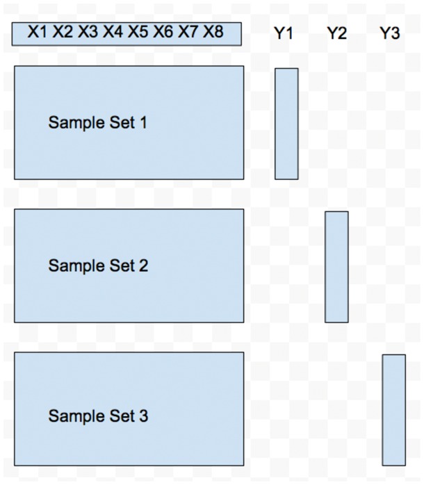
An example of multitasking learning

Fig. 2.

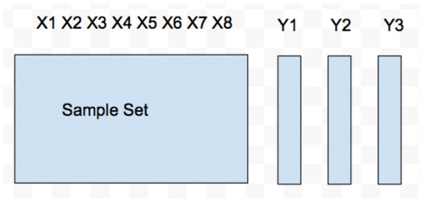
An example of multiple output regression

We can see that for the multitask learning problem, if we learn each task independently, we only use a small portion of the samples. If we model all the tasks at the same time, we leveraged the information from the complete set of samples and the improvement could be significant when the number of tasks is large. In the multiple output regression problem, although all the tasks share the same set of samples and there is no advantage on the sample size, the prediction performance could still be improved by the modeling the correlations among the tasks.

In this work, we adapt the state-of-the-art multitask learning algorithms and multiple output regression problems to solve the multiple trait prediction problem. For the multiple output regression problem, we conduct an iterative algorithm to learning the variable one at a time with others fixed. The objective function is convex when we only optimize one variable with others fixed, and therefore, efficient optimization is allowed. We observed that a direct application of these algorithms to the multiple trait prediction problem usually leads to poor least square error. We applied strategies such as centering the genotype matrix to improve the prediction performance. We showed that modeling all the traits together could improve the prediction compared with predicting each trait independently, especially for the correlated traits.

2 Preliminaries

Given the traditional encoding of genotypes as {0, 1, 2}, lots of techniques have been applied to the genetic trait prediction problem defined in Equation (1). Consider the typical situation for linear regression, where we have the training set $\mathit{y}\in {ℝ}^l,\mathit{x}\in {ℝ}^{l\times n}$, in a standard linear regression, we wish to find parameters ${\beta }_0,\mathbf{\beta }$ such that the sum of square residuals, ${\sum }_{i=1}^l{(y_i-{\mathbf{\beta }}_0-x_{i,·}^{\mathrm{\top }}\mathbf{\beta })}^2$, is minimized.

Many machine learning methods have been applied to the genetic single trait prediction problem, such as Elastic-Net, Lasso, Ridge Regression (Shaobing Chen et al., 1998; Tibshirani, 1994), Bayes A, Bayes B (Meuwissen et al., 2001), Bayes $C_{\pi }$ (Kizilkaya et al., 2010) and Bayesian Lasso (Legarra et al., 2011; Park and Casella, 2008). They could be applied to predict the multiple traits where each trait is predicted independently. In this work, we applied ridge regression (Hoerl and Kennard, 1970) for single trait prediction, which aims to minimize the following objective function.

$$\begin{array}{cc}\underset{}{\text{min}}& \left[{\displaystyle \sum _{i=1}^l{(y_i-x_i^T\mathbf{\beta })}^2}+\lambda {\displaystyle \sum _{j=1}^n{\beta }_j^2}\right],\end{array}$$ (2)

The solution of ridge regression is given by:

$$\begin{array}{c}\beta ={(X^{T}X+\lambda I)}^{-1}{X}^{T}y\end{array}$$ (3)

which is similar to the ordinal least square solution, but with the addition of a ‘ridge’ down the diagonal. Ridge regression has been shown to have certain bias as $-\lambda {(X^{T}X+\lambda I)}^{-1}\beta$. The unbiased version of rrBLUP (Ridge regression BLUP) (Meuwissen et al., 2001; Whittaker et al., 2000) is one of the most popular methods for genetic trait prediction. rrBLUP simply is ridge regression with a specific choice of λ in (2). Specifically, Meuwissen et al. (2001) assumes that the β coefficients are iid from a normal distribution such that ${\beta }_i\sim N(0,{\sigma }_{\beta }^2)$. Then the choice of $\lambda ={\sigma }_e^2/{\sigma }_{\beta }^2$ where ${\sigma }_e^2$ is the residual error. In this case, the ridge regression penalized estimator is equivalent to best linear unbiased predictor (BLUP) (Ruppert et al., 2003).

Many methods for multitrait prediction where all the traits are modeled together have also been proposed, such as multitrait GBLUP (Clark and van der Werf, 2013), Multitrait BayesA (Jia and Jannink, 2012), Bayesian multivariate antedependence model (Jiang et al., 2015). In multivariate models with m traits, marker effects on phenotypic traits were estimated from the mixed linear model below:

$$\begin{array}{c}y=u+{\displaystyle \sum _{j=1}^p{X}_j}{a}_j{\delta }_j+e\end{array}$$ (4)

where y is a n × m matrix with n samples and m traits, a_j is a $1\times m$ vector for the effects of the jth marker on all m traits which is assumed to be normally distributed $a_j\sim N(0,{\Sigma }_{{\alpha }_j}),{\Sigma }_{{\alpha }_j}$ is m × m variance-covariance matrix for the jth marker, e is a n × m matrix for residual error that follows a normal distribution.

In multitrait GBLUP (Cleveland et al., 2012), unstructured covariance matrix among traits was assumed and the relationship matrix derived from SNPs were fit in ASReml (Gilmour et al., 2009). The multitrait BayesA model (Jia and Jannink, 2012) assumes the prior of ${\Sigma }_{{\alpha }_j}$ follows a scaled inverse-Wishart distribution, which were given a flat prior and estimated from the data using the Metropolis algorithm to sample from the joint posterior distribution. Gibbs sampling and MCMC are applied to estimate the parameters. In the Bayesian multivariate antedependence model (Jiang et al., 2015), it is assumed that the adjacent markers are correlated as below:

$${\alpha }_j=\{\begin{array}{ll}{\delta }_j& j=1\\ t_{j,j-1}{\alpha }_{j-1}+{\delta }_j& j=2,\dots ,p\end{array}$$ (5)

where $t_{j,j-1}$ is the scalar antedependence parameter of α_j on ${\alpha }_{j-1}$. Again, the parameters are estimated via Gibbs sampling and MCMC.

3 Multitrait prediction

As we have discussed before, there are two types of multitrait prediction problem:

• For each trait, the genotype matrix is different: the problem can be formalized as a multitask learning problem.

• For each trait, the genotype matrix is the same: the problem can be formalized as a multiple output regression problem.

3.1 Multitask learning

Many algorithms have been proposed (Abernethy et al., 2006, 2009; Agarwal et al., 2010; Argyriou et al., 2007; Chen et al., 2012; Evgeniou and Pontil, 2004; Liu et al., 2009; Zhou et al., 2011) for the multitask learning problem. Here we mainly focused on four algorithms: Cluster-based MTL (CMTL) (Zhou et al., 2011), ${\ell }_1$-norm regularized MTL, ${\ell }_{2,1}$-norm regularized MTL (Liu et al., 2009) and Trace-norm Regularized MTL (Abernethy et al., 2009).

Lasso (Tibshirani, 1996) is a well-known method that uses the ${\ell }_1$-norm (or Lasso) regularizer to reduce model complexity and learn features. It can be easily extended for single task learning to multitask learning. The objective function for ${\ell }_1$-norm regularized MTL is based on least square lasso:

$$\begin{array}{c}{\min }_W{\displaystyle \sum _{i=1}^t|}|W_i^T{X}_i-Y_i|{|}_F^2+{\rho }_1\left|\right|W|{|}_1+{\rho }_{L_2}|\left|W\right|{|}_F^2\end{array}$$ (6)

where X_i denotes the input matrix of the ith task, Y_i denotes the ith trait, W_i is the coefficient matrix for task i, the regularization parameter ρ₁ controls sparsity and the optional ${\rho }_{L_2}$ regularization parameter controls the ${\ell }_2$-norm penalty. Note that both ${\ell }_1$-norm and ${\ell }_2$-norm penalties are used in Elastic Net.

Besides a simple ${\ell }_1$-norm regularizer, we could constrain all coefficient matrices to share a common set of features. This motivates the group sparsity, i.e. the ${\ell }_1/{\ell }_2$-norm, or ${\ell }_{2,1}$-norm, regularized learning (Liu et al., 2009). The objective function for ${\ell }_{2,1}$-norm regularized MTL is also based on least square lasso:

$$\begin{array}{c}{\min }_W{\displaystyle \sum _{i=1}^t|}|W_i^T{X}_i-Y_i|{|}_F^2+{\rho }_1\left|\right|W|{|}_{2,1}+{\rho }_{L_2}|\left|W\right|{|}_F^2\end{array}$$ (7)

where X_i denotes the input matrix of the ith task, Y_i denotes the ith trait, W_i is the coefficient matrix for task i, the regularization parameter ρ₁ controls sparsity and the optional ${\rho }_{L_2}$ regularization parameter controls the ${\ell }_2$-norm penalty. Notice the difference of the objective functions in Equations (6) ($\left|\right|W|{|}_1$) and (7) ($\left|\right|W|{|}_{2,1}$).

We could also constrain the coefficient matrices from different tasks to share a low-dimensional subspace, i.e. W is of low rank. By replacing the rank of W with trace norm $\left|\right|W|{|}_{*}=\sum _i{\delta }_i(W)$, the objective function becomes:

$$\begin{array}{c}{\min }_{W}L(W)+\gamma \left|\right|P|{|}_1\\ \text{subject to}:W=P+Q,\left|\right|Q|{|}_{*}<=\tau \end{array}$$ (8)

where the task coefficient matrices W is decomposed into two components: a sparse part P and a low-rank part Q.

The advantage of CMTL is that prior knowledge on the cluster structure of the traits can be embedded into the objective function. For our multitrait problem setting, we always know what are the traits and what they measured. Thus it is very often we know which traits are more correlated with each other. For example, fruit weight and fruit size are known to be highly correlated. These more correlated traits should be in one cluster. By leveraging such cluster information, we could improve the multitrait prediction algorithm. The objective function for CMTL is based on the spectral relaxed k-means clustering:

$${\min }_{W,F:F^{T}F=I_k}L(W)+\alpha (\text{tr}(W^{T}W)-\text{tr}(F^T{W}^{T}WF))+\beta \text{tr}(W^{T}W)$$ (9)

where k is the number of clusters and F captures the relaxed cluster assignment information. As the above objective function is not convex, a convex relaxation cCMTL is also proposed as below:

$$\begin{array}{c}{\text{min}}_{W}L(W)+{\rho }_1\eta (1+\eta )tr(W{(\eta I+M)}^{-1}{W}^T)\\ \text{subject to}:\text{tr}(M)=k,M\le I,M\in S_{+}^t,\eta =\frac{{\rho }_2}{{\rho }_1}\end{array}$$ (10)

Accelerated Projected Gradient (Zhou et al., 2011) is applied to optimize the above objective function.

3.2 Multiple output regression

Given a set of training data consisting of N samples, each sample is associated with a genotype matrix X of D-dimension and a trait matrix Y of C-dimension, the multioutput regression model is shown below:

$$Y=XB+E$$ (11)

where $B=[B_1,\dots ,B_c]$ is a D × C regression coefficient matrix, each element B_j is the vector of the regression coefficient for the jth trait. $E={[{\mathrm{ϵ}}_1,\dots ,{\mathrm{ϵ}}_N]}^T$ is an N × C matrix, where ${\mathrm{ϵ}}_i=({\mathrm{ϵ}}_{i1},\dots ,{\mathrm{ϵ}}_{iC})\in R^C$ denotes the residual errors on each trait prediction introduced by the ith sample.

Multiple output regression has been widely used in a variety of domains such as stock prices prediction, pollution prediction, etc. It was first noticed by Breiman (2000) and Friedman that through utilizing correlations between outputs the regression accuracy can be improved. In general there are two types of correlations: the task correlation and the noise correlation. Most of the work focus on modeling only one type of correlation, either task correlation or noise correlation. Some recent works (Cai et al., 2014; Rai et al., 2012) consider both types of correlation, which are shown to achieve better regression performance. The work of Rai et al. (2012) and Cai et al. (2014) are essentially the same in that they both aim to optimize the following objective function:

$$\begin{array}{c}\arg {\min }_{B,{\Omega }^{-1},{\Sigma }^{-1}}=\text{tr}((Y-XB){\Omega }^{-1}{(Y-XB)}^T)\\ -N\log \left|{\Omega }^{-1}\right|+{\lambda }_1\text{tr}(B{B}^T)+{\lambda }_2\text{tr}(B{\Sigma }^{-1}{B}^T)\\ -D\log \left|{\Sigma }^{-1}\right|+{\lambda }_3\text{tr}({\Omega }^{-1})+{\lambda }_4\text{tr}({\Sigma }^{-1})\end{array}$$ (12)

where $|.|$ denotes the determinant of a matrix.

The inverse covariance matrix ${\Omega }^{-1}$ couples the correlated noise across tags and similarly, ${\Sigma }^{-1}$ obtained relationships among the multiple tasks’ regression coefficients. Apparently, both ${\Omega }^{-1}$ and ${\Sigma }^{-1}$ are learnt from the training data rather than pre-defined prior knowledge. The last two terms $\text{tr}({\Omega }^{-1})$ and $\text{tr}({\Sigma }^{-1})$ are the regularizers, which impose the matrix variate Gaussian priors on both ${\Omega }^{-1/2}$ and ${\Sigma }^{-1/2}$ to solve the overfitting issue.

The objective function in Equation (12) of the multiple output regression model is not jointly convex in all variables but individually convex in each variable while others are fixed. Therefore, in order to optimize the objective function, an iterative algorithm is applied: (i) Fix ${\Omega }^{-1}$ and ${\Sigma }^{-1}$ and estimate B, (ii) Fix ${\Omega }^{-1}$ and B and estimate ${\Sigma }^{-1}$ and (iii) Fix ${\Sigma }^{-1}$ and B and estimate ${\Omega }^{-1}$. The process iterates and stops when the value of the objective function does not change or when the number of iterations exceeds a pre-defined threshold.

As the multiple output regression model is convex in each variable while others are fixed, when we optimize a variable, we can take the derivative of the variable to estimate its optimal value. To estimate B with fixed ${\Omega }^{-1}$ and ${\Sigma }^{-1}$, we set the derivative of B over the objective function as 0 and we obtain:

$$\begin{array}{c}2X^{T}XB{\Omega }^{-1}+2{\lambda }_{1}B+2{\lambda }_{2}B{\Sigma }^{-1}=2X^{T}Y{\Omega }^{-1}\\ \Rightarrow X^{T}XB+{\lambda }_{1}B\Omega +{\lambda }_{2}B{\Sigma }^{-1}\Omega =X^{T}Y\end{array}$$

Both works (Cai et al., 2014; Rai et al., 2012) applied the above algorithm. However, when optimizing B, the work (Rai et al., 2012) applies Kronecker product which generates a DC × DC matrix whose complexity might be high for large D and C. Then work Cai et al. (2014) MOR improved the complexity by applying Cholesky factorization and singular value decomposition and they showed that the efficiency of the optimization process can be significantly improved. Please refer to Rai et al. (2012) and Cai et al. (2014) for the details of the two approaches.

As ${\lambda }_1\Omega +{\lambda }_2{\Sigma }^{-1}\Omega$ is systemic and positive-definite, the Cholesky factorization is performed on it to produce lower triangular matrix P:

$$\begin{array}{c}{\lambda }_1\Omega +{\lambda }_2{\Sigma }^{-1}\Omega =P{P}^T\end{array}$$

By setting $X=U_1{\Sigma }_1{V}_1^T$ and $P=U_2{\Sigma }_2{V}_2^T$ be the SVD of X and P, respectively, we obtain the following:

$$\begin{array}{c}{V}_1{\Sigma }_1{U}_1^T{U}_1{\Sigma }_1{V}_1^{T}B+B{U}_2{\Sigma }_2{V}_2^T{V}_2{\Sigma }_2{U}_2^T=X^{T}Y\end{array}$$

By setting $\stackrel{\sim }{B}=V_1^{T}B{U}_2$ and $S=V_1^T{X}^{T}Y{U}_2$, we could obtain B as:

$$B=V_1\stackrel{\sim }{B}{U}_2^T$$

When optimize ${\Sigma }^{-1}$ with fixed ${\Omega }^{-1}$ and B, we set the derivative of ${\Sigma }^{-1}$ over the objective function as 0 and we obtain:

$$\begin{array}{c}{\lambda }_2{B}^{T}B-D\Sigma +{\lambda }_4{I}_C=0\\ \Rightarrow {\Sigma }^{-1}=(\frac{{\lambda }_2{B}^{T}B+{\lambda }_4{I}_C}{D})\end{array}$$

When optimize ${\Omega }^{-1}$ with fixed ${\Sigma }^{-1}$ and B, we set the derivative of ${\Sigma }^{-1}$ over the objective function as 0 and we obtain:

$$\begin{array}{c}{(Y-XB)}^T(Y-XB)-N\Omega +{\lambda }_3{I}_C=0\\ \Rightarrow {\Omega }^{-1}={(\frac{{(Y-XB)}^T(Y-XB)+{\lambda }_3{I}_C}{N})}^{-1}\end{array}$$

where I_C is an C × C identity matrix and $M^{-1}$ denotes the inverse matrix of the matrix M. The ${\lambda }_1,{\lambda }_2,{\lambda }_3$ are selected by cross-validation.

In Cai et al. (2014), dimensionality reduction is applied on both feature space and target (trait) space. Feature space is the space for all the features, which are the genotypes in our setting. Target space is the space for all the target variables, which are the multiple genetic traits in our setting. On feature space, PCA is applied to reduce the dimensionality. On target space, a regularizer is applied to reduce the dimensionality. In this work, we did not conduct dimensionality reduction as in the dataset we studied, the number of features (in thousands) and the number of traits (eight) are not very big.

Notice the MOR method without the task correlations and noise correlations can be reduced to a standard ridge regression. We observed that a direct application of the MOR method usually leads to poor accuracy, as the predicted values are usually far off the true values. In order to address this issue, we centered the input data matrix X as $\frac{X-\text{Mean}(X)}{\text{Std}(X)}$, where Mean(X) computes the column-wise mean of X, Std(X) computes the column-wise standard deviation of X. We call it Centered MOR. It turns out that the centering strategy significantly improved the least square error of MOR.

4 Results

4.1 Simulated data

We first simulate the data using the Equation (11). Recall that in this equation, $B=[B_1,\dots ,B_c]$ is a D × C regression coefficient matrix, each element B_j is the vector of the regression coefficient for the j-th trait. In order to add task correlation among all the B_j’s, we sample B_j’s from a standard normal distribution. Similarly, to add noise correlation, we sample the residual errors E from a standard normal distribution. The genotype matrix X is randomly sampled from the values [0, 1, 2]. The traits Y are then computed as $Y=XB+E$. We simulated four traits for 200 samples, each with 2000 markers. We repeat all the experiments 10 times and computed the average performance. To evaluate the performance of the prediction methods, we used r² (r-square, the square of the person’s correlation coefficient between the predicted trait values and the real trait values, a popular metric for genomic selection. For genomic selection, the r² is almost consistent with least square error). For r², the larger the better.

Notice we do not compare multitask learning and multiple output regression methods directly as they will be used in different scenarios. Multitask learning is used when we have unique set of samples for different traits. Multiple output regression is used when we have the same set of samples for all the traits.

4.1.1 Multitask learning

We randomly split the 200 samples into 4 subsets, each with 50 samples and one corresponding trait. All of these subsets share the same 2000 set of markers, with their corresponding genotype values. We tested the performance of the four multitask learning algorithms [Cluster-based MTL (CMTL), L1-norm regularized MTL, L2,1-norm regularized MTL, Trace-norm Regularized MTL] against the single trait ridge regression algorithm. Notice for the single trait algorithm, for each trait, we train ridge regression only on one subset of 50 samples. For CMTL, as we do not have specific clusters, we just randomly group two of the traits in one cluster and the other two in another cluster.

We show the results in Figure 3. We can see that the four multitask learning algorithms in general achieved much better results than that of the single trait ridge regression. This is reasonable as the single trait ridge regression only uses 50 samples for the prediction. The CMTL does not have any advantage over other methods as the traits are indeed not in clusters. The trace-norm MTL achieved the best results.

Fig. 3.

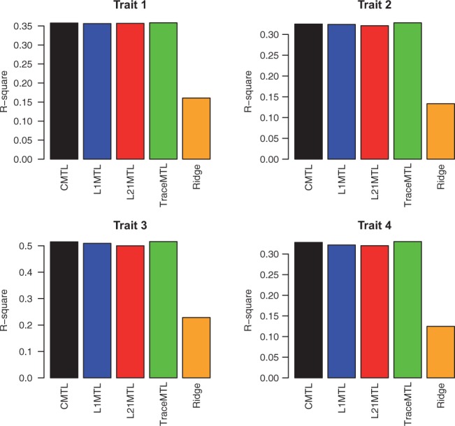
The r² of the four multitask learning algorithms versus the single trait ridge regression algorithm on the simulated data

4.1.2 Multiple output regression

Here we conducted 10-fold cross validation for each trait and we compare the performance of the the single trait prediction method: single trait ridge regression, the multiple output regression methods: the centered MOR method and the state-of-the-art multitrait prediction methods: the multitrait BayesA algorithm, the Bayesian multivariate antedependence model. We did not show the performance of MOR here as it in general has poor performance.

The results are shown in Figure 4. We can see that the multitrait algorithms have better performance than the single trait ridge regression does. The Bayesian multivariate antedependence model does not outperform BayesA in that we do not insert LD in our dataset. The centered MOR has the best performance. We also see that the multitrait prediction methods and multiple output regression methods made improvements on all four traits over the single trait prediction method. This is because all the four traits are correlated as they are sampled from the same standard normal distribution. As we will show later in the experiments on real data, when the traits are not correlated, multitrait prediction does not make obvious improvements.

Fig. 4.

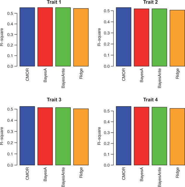
The r² of the centered MOR method, the multitrait BayesA algorithm, the Bayesian multivariate antedependence model versus the single trait ridge regression algorithm on the simulated data

4.2 Real data

Next we evaluate the performance of the multitrait prediction methods on a real plant dataset, the avocado dataset, which contains 8 traits, 160 samples and 2663 markers. The eight traits are: fruit weight, seed weight, fruit length, fruit width, fruit diameter, number of fruit (log), mesocarp weight and water loss percentage. From the name of the traits, we know which traits are more correlated with each other. We show the heat map of the correlation of these traits in Figure 5. Notice in the Figure there are two more traits ‘seed width’ and ‘seed length’. They are not included in the experiments. From the heat map, we can see that the first six traits are more correlated with each other and the last two traits are less correlated with the remaining traits.

Fig. 5.

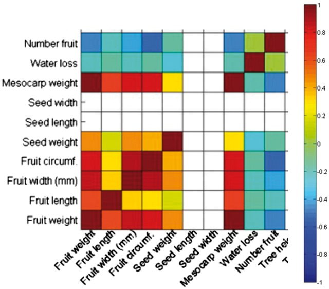
The heat map of the correlation of the eight traits

4.2.1 Multitask learning

We randomly divide the genotype matrix into eight subsets, each with 20 samples. Notice the eight genotype matrices share the same set of markers. For each subset, we keep only one trait for the corresponding samples in the subset. Therefore, we ended up with eight datasets, each with a single trait.

For single trait prediction, to predict the j-trait, we first train a predictive model on the jth dataset. Then we take all the other datasets as input and apply the predictive model on the other datasets to predict the jth trait for them. The predictive model we used here is ridge regression. For the multitrait prediction, we used four algorithms: Cluster-based MTL (CMTL), L1-norm regularized MTL, L2,1-norm regularized MTL and Trace-norm Regularized MTL. For CMTL, we applied our prior knowledge on the structure of the clusters, namely the traits fruit weight, fruit length, fruit width, fruit diameter are highly correlated and they should be in one cluster.

We compare the performance of the four multitask learning algorithms with the single trait prediction. We show the results in Figure 6. We can see the obviously the multitrait prediction significantly outperforms the single trait prediction, as the single trait prediction used only one-eighth of the complete data to predict each trait. We also observed that CMTL and the TraceNormMTL achieved better results than the other two MTL methods, as they conducted more complicated strategies rather than simple regularization. The TraceNormMTL achieved slightly better results than CMTL, indicating that reducing the original problem into a lower dimensional subspace is indeed an effective strategy when the dimensionality of the original problem is high.

Fig. 6.

The r² of the four multitask learning algorithms versus the single trait ridge regression algorithm

4.2.2 Multiple output regression

For the multiple output regression methods, as there is only one dataset, we conducted 10-fold cross validation. We evaluated the performance of the single trait prediction method: single trait ridge regression, the multiple output regression methods: the centered MOR method and the state-of-the-art multitrait prediction methods: the multitrait BayesA algorithm, the Bayesian multivariate antedependence model. Again we do not include MOR here as it has poor performance. Notice we do not include the multitrait GBLUP algorithm here as the two multitrait prediction methods have been shown to have superior performance over the multitrait GBLUP algorithm. The performance is again evaluated by the two metrics: r² and the least square error.

As we can see in Figure 7, both the multitrait and multiple output regression methods outperform single trait ridge regression. The centered MOR method achieved better performance than the ridge regression does, indicating that the centering strategy is critical for the genetic trait prediction problem. The centered MOR method also shows competitive performance compared with the multitrait prediction methods on most of the traits. Also we can observe that the improvement are mainly made on the first six traits, which are highly correlated with each other. For the last two traits, the multitrait prediction does not show advantages.

Fig. 7.

The r² of the centered MOR method, the multitrait BayesA algorithm, the Bayesian multivariate antedependence model versus the single trait ridge regression algorithm

5 Conclusions and future work

In this work, we studied the multitrait prediction problem where the multiple quantitative trait values of a set of samples are predicted from their corresponding genotypes. We modeled the problem from a machine learning perspective. We considered the problem as either a multitask learning problem or a multiple output regression problem. By adapting the state-of-the-art machine learning algorithms, we showed that the prediction accuracy can be improved by modeling all the traits together and we also showed that the machine learning methods are indeed very competitive with the existing statistical methods.

We also observed that the MOR method without the task correlations and noise correlations can be reduced into a standard ridge regression. From our previous study on single genetic trait prediction (Haws et al., 2015), we observed that rrBLUP (the unbiased version of ridge regression) achieves better performance than ridge regression does. In our future work, we would like to extend the MOR method to take the form of rrBLUP rather than ridge regression, which might improve its performance.

Conflict of Interest: none declared.

References

- Abernethy J. et al. (2006) Low-rank matrix factorization with attributes. arXiv Preprint Cs/0611124. [Google Scholar]
- Abernethy J. et al. (2009) A new approach to collaborative filtering: operator estimation with spectral regularization. J. Mach. Learn. Res., 10, 803–826. [Google Scholar]
- Agarwal A. et al. (2010) Learning multiple tasks using manifold regularization. Adv. Neural Inf. Process. Syst., 46–54. [Google Scholar]
- Argyriou A. et al. (2007) A spectral regularization framework for multi-task structure learning. Adv. Neural Inf. Process. Syst., 25–32. [Google Scholar]
- Breiman L. (2000) Randomizing outputs to increase prediction accuracy. Mach. Learn., 40, 229–242. [Google Scholar]
- Cai H. et al. (2014) Multi-output regression with tag correlation analysis for effective image tagging In: Lecture Notes in Computer Science., 8422, pp. 31–46. Springer, Berlin. [Google Scholar]
- Chen J. et al. (2012) Learning incoherent sparse and low-rank patterns from multiple tasks. ACM Trans. Knowl. Discov. Data (TKDD), 5, 22.. [DOI] [PMC free article] [PubMed] [Google Scholar]
- Clark S.A., van der Werf J. (2013) Genomic best linear unbiased prediction (gblup) for the estimation of genomic breeding values In: Genome-Wide Association Studies and Genomic Prediction, pp. 321–330. Springer, Berlin. [DOI] [PubMed] [Google Scholar]
- Cleveland M.A. et al. (2012) A common dataset for genomic analysis of livestock populations. G3: Genes— Genomes— Genetics, 2, 429–435. [DOI] [PMC free article] [PubMed] [Google Scholar]
- Evgeniou T., Pontil M. (2004) Regularized multi–task learning. In: Proceedings of the tenth ACM SIGKDD international conference on Knowledge discovery and data mining, pp. 109–117ACM.
- Gilmour A.R. et al. (2009) ASReml user guide release 3.0. VSN International Ltd, Hemel Hempstead, UK. [Google Scholar]
- Haws D.C. et al. (2015) Variable-selection emerges on top in empirical comparison of whole-genome complex-trait prediction methods. PloS One, 10, e0138903.. [DOI] [PMC free article] [PubMed] [Google Scholar]
- Hayes B.J. et al. (2009) Genomic selection in dairy cattle: Progress and challenges. J. Dairy Sci., 92, 433–443. [DOI] [PubMed] [Google Scholar]
- Heffner E.L. et al. (2009) Genomic selection for crop improvement. Crop Sci., 49, 1–12. [Google Scholar]
- Hoerl A.E., Kennard R.W. (1970) Ridge regression: biased estimation for nonorthogonal problems. Technometrics, 12, 55–67. [Google Scholar]
- Jannink J.-L. et al. (2010) Genomic selection in plant breeding: from theory to practice. Brief. Funct. Genomics, 9, 166–177. [DOI] [PubMed] [Google Scholar]
- Jia Y., Jannink J.-L. (2012) Multiple-trait genomic selection methods increase genetic value prediction accuracy. Genetics, 192, 1513–1522. [DOI] [PMC free article] [PubMed] [Google Scholar]
- Jiang J. et al. (2015) Joint prediction of multiple quantitative traits using a bayesian multivariate antedependence model. Heredity, 115, 29–36. [DOI] [PMC free article] [PubMed] [Google Scholar]
- Kizilkaya K. et al. (2010) Genomic prediction of simulated multibreed and purebred performance using observed fifty thousand single nucleotide polymorphism genotypes. J. Anim. Sci., 88, 544–551. [DOI] [PubMed] [Google Scholar]
- Lande R., Thompson R. (1990) Efficiency of marker-assisted selection in the improvement of quantitative traits. Genetics, 124, 743–756. [DOI] [PMC free article] [PubMed] [Google Scholar]
- Legarra A. et al. (2011) Improved lasso for genomic selection. Genet. Res., 93, 77. [DOI] [PubMed] [Google Scholar]
- Liu J. et al. (2009) Multi-task feature learning via efficient l 2, 1-norm minimization. In: Proceedings of the twenty-fifth conference on uncertainty in artificial intelligence, pp. 339–348AUAI Press.
- Meuwissen T.H.E. et al. (2001) Prediction of total genetic value using genome-wide dense marker maps. Genetics, 157, 1819–1829. [DOI] [PMC free article] [PubMed] [Google Scholar]
- Park T., Casella G. (June 2008) The bayesian lasso. J. Am. Stat. Assoc., 103, 681–686. [Google Scholar]
- Rai P. et al. (2012) Simultaneously leveraging output and task structures for multiple-output regression. Adv. Neural Inf. Process. Syst., 3185–3193. [Google Scholar]
- Rincent R. et al. (2012) Maximizing the reliability of genomic selection by optimizing the calibration set of reference individuals: Comparison of methods in two diverse groups of maize inbreds (zea mays l.). Genetics, 192, 715–728. [DOI] [PMC free article] [PubMed] [Google Scholar]
- Ruppert D. et al. (2003) Semiparametric Regression In: Cambridge Series in Statistical and Probabilistic Mathematics. Cambridge University Press, New York, NY. [Google Scholar]
- Shaobing Chen S. et al. (1998) Atomic decomposition by basis pursuit. SIAM J. Sci. Comput., 20, 33–61. [Google Scholar]
- Tibshirani R. (1994) Regression shrinkage and selection via the lasso. J. R. Stat. Soc. Ser. B, 58, 267–288. [Google Scholar]
- Tibshirani R. (1996) Regression shrinkage and selection via the lasso. J. R. Stat. Soc. Ser. B (Methodological), 267–288. p [Google Scholar]
- Whittaker J.C. et al. (2000) Marker-assisted selection using ridge regression. Genet. Res., 75, 249–252. [DOI] [PubMed] [Google Scholar]
- Xu Y., Crouch J.H. (2008) Marker-assisted selection in plant breeding: from publications to practice. Crop Sci., 48, 391–407. [Google Scholar]
- Zhou J. et al. (2011) Clustered multi-task learning via alternating structure optimization. Adv. Neural Inf. Process. Syst., 702–710. [PMC free article] [PubMed] [Google Scholar]