

Abstract
Motivation: Protein–protein interactions are a key in virtually all biological processes. For a detailed understanding of the biological processes, the structure of the protein complex is essential. Given the current experimental techniques for structure determination, the vast majority of all protein complexes will never be solved by experimental techniques. In lack of experimental data, computational docking methods can be used to predict the structure of the protein complex. A common strategy is to generate many alternative docking solutions (atomic models) and then use a scoring function to select the best. The success of the computational docking technique is, to a large degree, dependent on the ability of the scoring function to accurately rank and score the many alternative docking models.
Results: Here, we present ProQDock, a scoring function that predicts the absolute quality of docking model measured by a novel protein docking quality score (DockQ). ProQDock uses support vector machines trained to predict the quality of protein docking models using features that can be calculated from the docking model itself. By combining different types of features describing both the protein–protein interface and the overall physical chemistry, it was possible to improve the correlation with DockQ from 0.25 for the best individual feature (electrostatic complementarity) to 0.49 for the final version of ProQDock. ProQDock performed better than the state-of-the-art methods ZRANK and ZRANK2 in terms of correlations, ranking and finding correct models on an independent test set. Finally, we also demonstrate that it is possible to combine ProQDock with ZRANK and ZRANK2 to improve performance even further.
Availability and implementation: http://bioinfo.ifm.liu.se/ProQDock
Contact: bjornw@ifm.liu.se
Supplementary information: Supplementary data are available at Bioinformatics online.
1 Introduction
Protein–protein interactions are crucial in almost all biological processes. To understand the mechanism of protein–protein interaction, the structure of the protein complex is essential. Despite massive efforts in structure determination the majority of protein complexes are not and will never be available in the PDB (Berman et al., 2000). Thus, there is a great need for computational methods that are able to build models of protein complexes using docking.
Constructing models of protein complexes is a fundamental challenge in structural biology and despite years of investigation is still unsolved. The problem can be divided into sampling and scoring, where sampling is the problem of generating realistic docking models, and scoring is the problem of identifying the correct docking models among many incorrect ones. A number of different approaches have been applied to this problem ranging from composite scoring describing the physics (Dominguez et al., 2003; Cheng et al., 2007; Lyskov and Gray, 2008; Pierce and Weng, 2007, 2008) to methods derived from the statistics of structural databases (Geppert et al., 2010; Liu and Vakser, 2011; Pons et al., 2011), methods based on interface composition and geometry (Chang et al., 2008; Khashan et al., 2012; Mitra and Pal, 2010) or complementarity (Gabb et al., 1997; Lawrence and Colman, 1993; McCoy et al., 1997) and methods based on machine learning (Bordner and Gorin, 2007; Chae et al., 2010). The different approaches provide different aspects of docking model quality and could potentially result in higher performance when combined together (Moal et al., 2013).
The multitude of approaches applied to the scoring problem highlights the difficulty in scoring protein docking models. At one end there are features that serve as critical filters for complex formation, like shape complementarity (Lawrence and Colman, 1993) while on the other end, there could be features that might largely vary even among good-quality models. It is, for instance, fairly easy to generate completely incorrect docking models with good shape complementarity, as the van der Waals interactions contribute favorably to the scoring function used in sampling. Another problem in scoring docking models in general occurs when the docking models have been generated using different force fields, which is often the case, in particular in the scoring part of CAPRI (Lensink and Wodak, 2014). In this case, an almost perfectly correct model scoring well in one force field, might contain some small clashes in some other force field. Of course, it might be possible to refine the docking models and remove the clash. However, this is time-consuming and it might be worthy only if the model is correct, and as most docking models are incorrect it would be better if promising cases could be quickly detected without the need for extensive calculations. For instance, the use of coarse-grained scoring function, which are less sensitive to local errors than all-atom scoring functions (Viswanath et al., 2013) is one such example. However, it is likely that other features such as electrostatic balance at the interface, solvation, amino acid composition at the interface, etc. are also important to discriminate incorrect and correct docking models and finding the right balance between features is a highly non-trivial task.
In this study, we present the development of an algorithm, ProQDock, that predicts the quality of docking models using structural information, scoring functions and the predicted features were combined using a support vector machine (SVM). The method is optimized on realistic docking models to predict the DockQ score (Basu and Wallner, 2016), of the corresponding model. DockQ is a score between 0 and 1, which is similar to IS-score (Gao and Skolnick, 2011) in its design, but optimized to reproduce the CAPRI classification (Lensink et al., 2007).
2 Methods
2.1 Training set
To train ProQDock, two benchmark sets of protein–protein docking models were used, the ‘CAPRI' set (Lensink and Wodak, 2014), which contains 19 013 models from 15 targets submitted to the CAPRI scoring experiment, and the ‘MOAL' set (Moal et al., 2013) containing 56 015 models for 118 targets from the docking Benchmark 4.0 (Hwang et al., 2010) using SwarmDock (Torchala et al., 2013) to generate the models (generously provided by authors of Moal et al.). The targets T36 (PDB ID: 2W5F) and T38 (3FM8) from the CAPRI set were discarded because they lacked at least a single acceptable (or better) model, resulting in 17 777 models from 13 targets.
The constructions of the two benchmark sets are completely different: the CAPRI set is based on docking model submitted to CAPRI, which contains predictions from many different methods, while the MOAL set contains models generated with only one method. In that respect, the CAPRI set is probably more realistic, as it contains models made with a variety of methods. On the other hand, the number of models and in particular the number of targets are small in the CAPRI set. Thus, to achieve a larger and more balanced set, the CAPRI set and MOAL set were combined into one set, 'CnM' (CAPRI and MOAL), to be used in training ProQDock using cross-validation (see below). The combined data set contained 73 792 docking models from 131 targets and is available at http://bioinfo.ifm.liu.se/ProQDock/.
2.2 Independent test set, BM5
Although, training of the machine learning algorithm was performed using a cross-validation procedure, the efficacy of ProQDock was independently tested on a dataset based on 55 new docking targets added to the Benchmark 4.0 in its updated version, Benchmark 5.0 (Vreven et al., 2015). In total, 25 985 docking models generated with SwarmDock (Torchala et al., 2013) for these 55 targets were again kindly provided by the authors of Vreven et al. (2015).
2.3 Native structures test set
To test the ability of ProQDock on native structure and to suggest a range of predicted values characteristic of native protein–protein complexes. A set consisting of 1879 co-crystallized interacting native structures with resolution better than 2 Å, and no missing backbone atoms were assembled using the ‘Build Database' option from Dockground (Anishchenko et al., 2014).
2.4 Cross-validation test sets
Five-fold cross-validation was used for training and assessing performance. To this end the training set targets were divided in five parts (cross-validation test sets) with no homologous proteins between them, four were used for training while testing the remaining one. This was performed for each of the five parts to get predictions for the whole set. All homologous proteins were placed in the same cross-validation test set, to ensure that the training and testing data for the same round of cross-validation did not contain any homologous between them. Blastclust (Altschul et al., 1990) was used to cluster homologous sequences from all complexes using a strict criteria 20% sequence similarity over at least 50% sequence coverage (-L 0.5 -S 20). Two complexes were considered homologous if at least one of the partners was homologous and placed in the same cluster. Finally, all clusters were grouped into five with approximately the same number of targets, with the total number of models spanning from 13 058 to 15 227 and the ratio of acceptable (or better) to incorrect models, spanning a range of 0.016 to 0.14. Neither different groupings (5-fold) nor jack-knifing (leave-one-out) did affect the performance (data not shown). A similar cross-validation strategy was used in the related problem of binding affinity predictions (Marillet et al., 2016) having similar number of high-level features (11 compared to 13 in the current study) and similar number of available native target complexes (144 compared to 131).
2.5 Target function
The target function should ideally reflect the true quality of a given protein–protein docking model. The state-of-the-art quality measure in docking, established by the CAPRI community, is to use three distinct though related measures, Fnat, LRMS and iRMS (Méndez et al., 2003). Fnat is the fraction of native interfacial contacts preserved in the model, LRMS the root mean square deviation for the smaller chain (ligand) after superposition of the larger chain (receptor) and iRMS is the RMS deviation of the interfacial atoms. By applying various ad hoc cutoffs on these three measures, protein–protein docking models are classified as ‘incorrect', ‘acceptable', 'medium' or 'high' quality. To avoid this classification scheme, we recently developed DockQ (Basu and Wallner, 2016), which combines Fnat, LRMS and iRMS into a continuous score between [0,1], reflecting no similarity (0) to perfect similarity (1). It was demonstrated that the continuous DockQ score can almost completely recapitulate the CAPRI classification into incorrect, acceptable, medium and high quality (94% average PPV at 90% Recall) using the following cutoffs: incorrect <0.23, acceptable [0.23,0.49), medium [0.49,0.8), high >0.8. Thus, DockQ is essentially a higher resolution version of the already established state of the art in the docking field and used as the target function to train ProQDock.
2.6 SVM Training
The Support Vector Regression module in the SVMlight package (Joachims, 2002) was used to train ProQDock using 5-fold cross-validation with radial basis function (RBF) kernel. The trade-off between training error and margin, C, and the RBF γ parameter were optimized using a grid search in the ranges; C from 2−15 to 210, and γ from 2−10 to 210, in log2 steps, maximizing the cross-validated Pearson's correlation coefficient. The epsilon width of tube for regression was kept at 0.1 (default). Because there were large imbalances in the number of acceptable (positive example) and incorrect (negative) models, the cost factor (-j flag) option of SVMlearn was set to the ratio of 'incorrect-to-acceptable' models, so that the training errors on negative examples could be outweighed by errors on positive examples (Morik et al., 1999). Rosetta energy terms and CPM were scaled between 0 and 1 to improve convergence using logistic scaling: Scaled(E) = 1/(1 + exp(-k(E-E0)), where E0 is the midpoint of the sigmoid and k the steepness of the sigmoid curve. E0 and k were optimized by estimating the cumulative distribution function, cdf(E), for a given training feature using the kernel smoothing function ksdensity in MATLAB. E0 was chosen as the midpoint of the data, i.e. cdf(E0) = 0.5, and k to cover at least 99% of the data, by selecting the lowest k (largest coverage) that made the Scaled(E) pass through the points (E1, 0.01) or (E2, 0.99) where cdf(E1) = 0.01 and cdf(E2) = 0.99.
2.7 Training features
A number of different features that describe either some specific structural properties of protein–protein interfaces or the overall protein structural integrity and quality were calculated and used for training ProQDock. The features are described in detail below.
2.7.1. Shape complementarity
The complementary in shape of protein–protein interface is a necessary condition for binding. Shape complementary (Sc) of a protein–protein interface (Lawrence and Colman, 1993) was calculated using the program Sc part of CCP4 package (Winn et al., 2011). Sc is defined in a range from −1 to 1 corresponding to anti- and perfectly correlated surfaces, respectively.
2.7.2. Electrostatic complementarity
The electrostatic character of native protein–protein interfaces is generally associated with anti-correlated surface electrostatic potentials (McCoy et al., 1997), reflected in positive values of the term, electrostatic complementarity (EC). First, the molecular surface (Connolly, 1983) was generated individually for both the partner molecules using the software EDTSurf (Xu and Zhang, 2009), with the scale factor for the optimum fit of the molecule in a bounding box set to 1.0. The protein–protein interface atoms were defined as atoms having a net (non-zero) change in solvent accessible surface area calculated for the bound and unbound state by NACCESS (Hubbard and Thornton, 1993). Hydrogen atoms were geometrically fitted by REDUCE (Word et al., 1999), partial charges and atomic radii were assigned by the AMBER94 all-atom molecular-mechanics force field (Cornell et al., 1995). DelPhi (Li et al., 2012) was used to compute the electrostatic potential for each surface point (buried on association) at the interface, iteratively solving the linearized version of the Poisson-Boltzman equation. From the electrostatic surface potentials generated at both interfaces, EC was calculated precisely according to the original methodology (McCoy et al., 1997), which was also used to probe electrostatic complementarity (Em) within protein interiors (Basu et al., 2012). The internal dielectric within the interior and buried interfaces of proteins were generally considered to be low (ε = 2), although, the more advanced multi-dielectric Gaussian smoothening method (Li et al., 2013) was also adapted in a trial calculation in all native structures (DB3). Both methods (single and multi-dielectric) resulted in similar EC values (rmsd: 0.15, Pearsons Correlation: 0.94). Similar to Sc, EC is defined from −1 to 1, and it approaches 1 with increasing matching (anti-correlation) of surface electrostatic potential generated on the same surface, owing to two complementary set of atoms, whereas a negative EC reflects unbalanced electric fields at the interface.
2.7.3. Relative size of the interface (nBSA, Fintres)
Neither the shape (Sc) nor EC, described above, takes the size of the interface into account. Native complexes have been found to exist spanning a wide range from small (< 10 amino acids) to large interfaces (Basu et al., 2014b). Also, only a few atoms at the interface can give rise to very high Sc (Lawrence and Colman, 1993) depending on how good their shapes correlate (e.g. 2FPE: 39 atoms, Sc: 0.83, 1D2Z: 14 atoms, Sc: 0.57). Thus, both Sc and EC should be coupled with additional features measuring the size of the interface. Following similar formulations to that of the 'Overlap' parameter (Banerjee et al., 2003) introduced for protein interiors, here, two related yet independent measures were calculated to account for the size of the interface: (i) the normalized buried surface area (nBSA), which measures the fraction of exposed surface area buried upon association, and (ii) the fraction of residues buried at the interface (Fintres).
2.7.4. Joint conditional probability of Sc, EC given nBSA
The joint conditional probability of Sc and EC given the actual size of the interface obtained from native protein-protein interactions (PPI) complexes was added as a separate feature. A similar function was shown to be successful in fold-recognition (Basu et al., 2012). To this end, nBSA, Sc and EC were computed in a database containing 1879 native structures from DOCKGROUND (see Section 2). Based on the distribution of nBSA, interfaces were classified as small (nBSA ≤ 0.05), medium (0.05 < nBSA ≤ 0.10) and large (nBSA > 0.10). Distributions of Sc and EC were divided into intervals of 0.05 and their normalized frequencies calculated. For a given complex, CPM is the joint conditional probability of finding its interface within a certain range of Sc and EC given its size (nBSA), i.e. CPM = log(P(Sc|nBSA) + log(P(EC|nBSA)), where P(Sc|nBSA) and P(EC|nBSA) are the probabilities of finding an interface within a certain range of Sc and EC values conditioned by its relative size, nBSA. CPM was set to 0 if P(Sc|nBSA) or P(EC|nBSA) was 0 to avoid the log score being undefined.
2.7.5. Link density
To capture the density of atomic contacts at the interface, the link density (Ld) measure was implemented (Basu et al., 2011). Ld is defined as the ratio of the actual number of links at the interface to the theoretical maximum number of links, where a link is pair of interacting residues from two chains defined as having at least one pair of heavy atoms within 6Å. If M and N residues are found to be at the interface from chain A and B, respectively, then the maximum number of links is M × N.
2.7.6. Interface contact preference score
It is well known that particular inter-residue contacts are preferred at protein interfaces (Lo Conte et al., 1999). To account for this fact, a Contact Preference Score (CPscore) was derived by training a SVM to predict DockQ using inter-residue contact information alone. The training was performed using the 5-fold cross-validation sets, as described above, but before the training of ProQDock. The inter-residue contact information was encoded as the fraction of any residue-residue contact, weighted by a contact preference weight available in the literature (Glaser et al., 2001). All possible combinations of amino acid pairs comprise 210 residue–residue contacts. Inter-residue contacts were defined as any two side-chain heavy atoms (CA for Glycine) within 10Å between the two molecules. This cutoff was deliberately kept somewhat relaxed in consistency with the measure iRMS (Méndez et al., 2003), to account for all possible combination of residue pairs at the interface.
2.7.7. Accessibility score
The expected distribution of amino acid residues with respect to burial was estimated by the accessibility score (rGb—residue Given burial) as detailed in an earlier publication (Basu et al., 2014a). rGb measures the propensity of a particular amino acid residue given a specific solvent accessibility. First, the burial of solvent exposure for individual residues were estimated by the ratio of ASA of the amino acid X in the polypeptide chain to that of an identical residue located in a Gly-X-Gly peptide fragment with a fully extended conformation. The hydrophobic burial profile for a given PPI model was then compared with an equivalent native profile. The rGb values for native PPI complexes are in the range of 0.059 (±0.022) (Basu et al., 2014b), where values 2σ below the mean (here 0.011) correspond to partially unfolded structures with hydrophobic residues being completely exposed to the solvent (Basu et al., 2014a). The consideration of rGb as an all-atom feature was also motivated by recent studies, emphasizing the plausible role of the non-interacting protein surface in modulating the binding affinity of potential protein–protein interactions (Visscher et al., 2015), primarily owing to solvation effect.
2.7.8. Protein model accuracy (ProQ2)
The overall structural quality of the whole complex, taken to be a folded pseudo-unimolecule, was estimated by the protein quality predictor ProQ2 (Uziela and Wallner, 2016) shown to be one of the best protein quality predictors in CASP11 quality assessment category (Kryshtafovych et al., 2015).
2.7.9. Rosetta energy terms (rTs, Isc, Erep, Etmr)
The structure integrity and quality of packing was assessed by scoring each protein–protein docking model using Rosetta all-atom energy function with the 'talaris2013' weight set (O’Meara et al., 2015). Before scoring, the side chains of each protein–protein docking model were rebuild. Ideally, each model should have been subjected to a full Rosetta relax or at least a short minimization to relieve potential backbone clashes. However, it turned out that even only side chain rebuild and minimization was too time-consuming (>5 min per model in some cases), given that the aim of the current study is to develop a tool that should be able to score thousands of models.
The Rosetta total score (rTs), the interface energy (Isc), the van der Waals repulsive term (Erep) and the total score minus the repulsive term (Etmr) were used. The reason to separate the repulsive term was that even a small clash might give high contributions to the total energy, obfuscating potential good energy terms. Because all terms except Isc depend on the chain length (the probability of higher number of interactions increases with chain length), before SVM training all terms except Isc were normalized by the length of the target complex. Isc was not normalized because stability in terms of binding energy is not necessarily a function of the interface size, and there might be instances where a small but stable interface could be energetically more favorable than a larger (unstable) interface.
2.8 ZRANK and ZRANK2
The knowledge-based all atom energy terms ZRANK (Pierce and Weng, 2007) and ZRANK2 (Pierce and Weng, 2008) were also computed, primarily for comparing the SVM results, but also for use in the hybrid method ProQDockQZ. Both ZRANK and ZRANK2 include van der Waals, electrostatics (Coulomb, using distance dependent dielectric) and desolvation energy terms. In addition, ZRANK2 includes the IFACE term, an interface statistical potential (Mintseris et al., 2007). ZRANK was primarily designed to re-rank initial docking predictions from ZDOCK, while ZRANK2 was designed toward refinement of protein docking models, in conjunction with RosettaDock (Gray et al., 2003). Besides the IFACE potential, the weight for the repulsive van der Waals is significantly smaller for ZRANK, making it less sensitive to small clashes compared with ZRANK2.
2.9 Evaluation Measures
Apart from calculating direct correlation (Pearson's) between scoring function and the quality measure (DockQ) used as target function, performance was also measured by Receiver Operating Characteristic (ROC) curves and ability to correctly rank models.
2.9.1. ROC curves
Performance of classifying protein–protein docking models as acceptable or better according to the CAPRI classification was evaluated based on true-positive rate (TPR, also known as recall), and false-positive rate (FPR)
where TP is the number of protein–protein docking models with a CAPRI classification acceptable or better correctly predicted as positive (true positives); FP is the number of misclassified negative cases (false positive); TN is the number of correctly predicted negatives (true negatives); FN is the number of misclassified positive cases (false negative). For any prediction method, ROC curves (TPR versus FPR) were constructed by sorting the prediction from good to bad and calculate TP, FP, FN, TN for all possible cutoffs for positive prediction. The area under the curve (AUC) was calculated using the trapezoidal numerical integration function trapz in MATLAB.
2.9.2. Ranking ability
The ability to properly rank models was measured by counting the number of correct models, defined as acceptable or better, ranked at top 1; within top 5, top 10 and top 100 by any given method. This measure is identical to the measure in a recent benchmark of scoring metrics for docking (Moal et al., 2013).
3 Results and Discussion
The aim of this study was to develop a method, ProQDock, that is capable of predicting the absolute quality of protein–protein docking models. The main idea is to calculate high-level features (Table 1) from each protein–protein docking model and use these features to predict the correctness of the protein–protein docking model as measured by the DockQ score (see Section 2).
Table 1.
Description of ProQDock training features
| Features | Feature description |
|---|---|
| nBSA | Normalized buried surface area |
| Fintres | Fraction of residues at the interface |
| rGb | Accessibility score |
| CPscore | Contact Preference score |
| Ld | Link Density at the interface |
| Sc | Shape Complementarity at the interface |
| EC | Electrostatic Complementarity at the interface |
| CPM | Joint Conditional Probability of Sc, EC given nBSA |
| ProQ2 | Protein model quality prediction |
| ISca | Rosetta interface energy |
| rTsa | Rosetta total energy |
| Erepa | Rosetta repulsive term |
| Etmra | Rosetta total energy minus repulsive |
aEnergy terms, lower scores are better.
3.1 Development of ProQDock
SVM training was performed using 5-fold cross-validation using different subsets of features in Table 1 to predict the DockQ score on the combined CnM dataset and the performances were primarily evaluated by their Pearson's Correlation values (versus DockQ). Best individual correlations were obtained for EC (0.24) and nBSA (0.17) (Fig. 1). Features were then categorized into interface (Int1, Int2) and all-atom (All1, All2) features according to their physico-chemical description, finally leading into four groups—Int1: size and packing of the interface {nBSA, Fintres, Sc, Ld}; Int2: electrostatics, binding energy and composition of the interface {EC, CPM, CPscore, ISc}; All1: solvation and overall quality of the whole complex {rGb, ProQ2}; All2: the Rosetta all-atom energy terms {rTs, Erep, Etmr}. Each group had better correlations than any of their constituting features (Fig. 1). Merging the interface and the all atom features, correlations were further improved to 0.35 for {Int1 + Int2} and 0.25 for {All1 + All2}, respectively. Finally, combining all features, it was possible to improve the performance to 0.49 for ProQDock (Fig. 1). The correlations indicate that the interface features are more influential though the all atom features are also necessary to improve the overall performance.
Fig. 1.
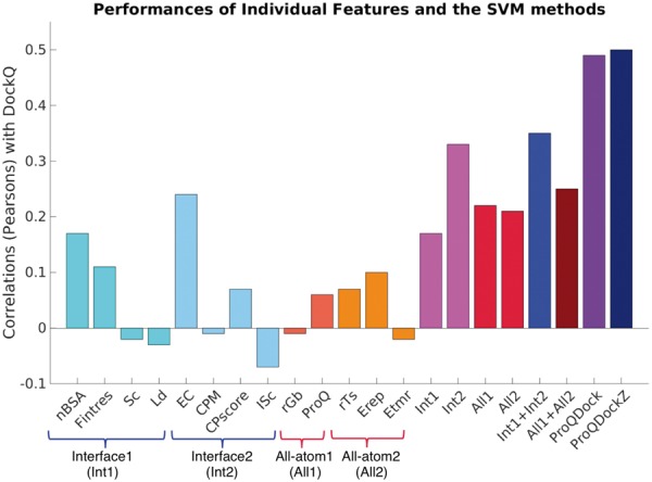
Correlations with DockQ for different training features and their combinations
In addition, ProQDock was combined with the external energy terms, ZRANK (Pierce and Weng, 2007) and ZRANK2 (Pierce and Weng, 2008) (ProQDockZ), using a linear weighted sum optimized on the CnM set. ZRANK2 and ZRANK were chosen primarily as independent methods to benchmark the performance of ProQDock because ZRANK2 was one of the best methods in a recent benchmark of docking scoring functions (Moal et al., 2013). To analyze if combining different complementary scoring functions would yield better performance, the hybrid method, ProQDockZ, was also included in the benchmark as a comparison. Indeed, the combined method further improved the correlation slightly from 0.49 for ProQDock to 0.50 for ProQDockZ (Fig. 1 and Table 2).
Table 2.
Correlations with DockQ on different datasets
| Methods | CnM n = 73 792 | CAPRI n = 17 777 | MOAL n = 56 015 | BM5 n = 25 985 |
|---|---|---|---|---|
| ProQDock | 0.49 ±0.01 | 0.55 ±0.01 | 0.34 ±0.01 | 0.37 ±0.01 |
| ProQDockZ | 0.50 ±0.01 | 0.57 ±0.01 | 0.36 ±0.01 | 0.38 ±0.01 |
| ZRANK | −0.31 ±0.01 | −0.39 ±0.02 | −0.21 ±0.01 | −0.22 ±0.02 |
| ZRANK2 | −0.20 ±0.01 | −0.25 ±0.02 | −0.31 ±0.01 | −0.33 ±0.01 |
Confidence intervals are at 99% level.
3.2 Benchmark on cross-validated data
The performances of ProQDock and ProQDockZ were compared with ZRANK and ZRANK2 on the CnM set by analyzing correlations (Table 2) as well as the ranking ability of each method and ROC curves (Fig. 2). Out of 131 targets, ProQDockZ, ProQDock, ZRANK2 and ZRANK could detect a correct (acceptable or better) model in 36, 33, 32 and 23 cases at the top rank, respectively, while, in 65, 61, 60 and 40 cases, at least one correct model was detected within top 10 ranks. Thus, the ranking ability are similar for ProQDock and ZRANK2, whereas the combined method ProQDockZ is slightly better than both methods (Fig. 2A). A more detailed analysis using ROC curves revealed that ProQDock (AUC = 0.87) in fact performed significantly better than both ZRANK (AUC = 0.71) and ZRANK2 (AUC = 0.75). By using a ProQDock score of 0.23 for correct predictions, ProQDock is able to find 80% of the correct models (TPR = 0.8 in Fig. 2B) at 20% FPR. The combined method, ProQDockZ, further enhanced the overall prediction ability (AUC = 0.88), finding slightly more true positives for all FPRs (Fig. 2B).
Fig. 2.
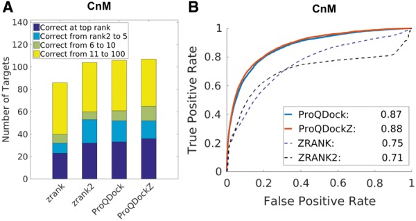
CnM performance measured by (A) the ability to rank a model with quality acceptable or better among top 1, 5, 10 and 100 and (B) ROC curves; the AUC values are given in the legend
Both ProQDock and ProQDockZ correlate significantly better than ZRANK and ZRANK2 with the true quality measure DockQ (Table 2). ProQDockZ has a small but significantly better correlation than ProQDock. ZRANK has a better correlation than ZRANK2 despite the fact that ZRANK2 has been reported to have the better performance (Moal et al., 2013). To explain the reason for this, correlations were calculated separately for the CAPRI and MOAL part of the CnM set (Table 2). This shows that ZRANK2 has a better correlation than ZRANK on MOAL but worse on CAPRI. This is because the CAPRI set contains docking models created using different methods, where many of the models have not been energy minimized and hence will contain more clashes, as opposed to the models in the MOAL set, where all models were energy minimized using SwarmDock (Torchala et al., 2013) (see Erep term for MOAL and CAPRI in Supplementary Figs S1 and S2). A major difference between ZRANK and ZRANK2 is that ZRANK2 has a harder repulsive term, which makes it more sensitive for models without clashes but obviously less sensitive on models with clashes. ROC curves for CAPRI and MOAL also illustrate this behavior (Fig. 3). ZRANK is better than ZRANK2 on CAPRI and vice versa on MOAL, while ProQDock performs much better than both on CAPRI; similar to ZRANK2 and much better than ZRANK on MOAL. Demonstrating that ProQDock can capture both coarse-grained and full-atom detail needed to perform well on both sets. As shown on the combined set, CnM, ProQDockZ is marginally better than both ProQDock and ZRANK2 on both subsets. The P-values corresponding to the difference in correlations (versus DockQ) between both ProQDock and ProQDockZ are < 0.01 over both ZRANK and ZRANK2, suggesting that the correlations are significantly better at 99% confidence level implying definite improvement in performance (Table 2). This is true for both, the cross-validated (CnM) and the independent benchmark (BM5).
Fig. 3.
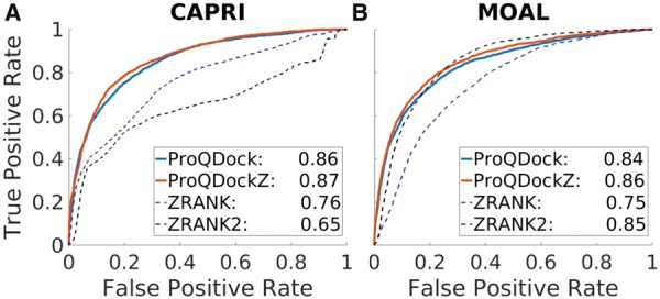
ROC curves for the (A) CAPRI part and (B) MOAL part of the CnM set. AUC values in the legend
3.3 Performance on independent test set BM5
The performance of the different scoring functions was further tested on the independent dataset, BM5, consisting of 25 985 models from 55 targets. In ranking, ProQDock and ProQDockZ could detect a correct (acceptable or better) model in 8 and 8 targets at the top rank, respectively; while, ZRANK and ZRANK2 could detect 4 and 10 (Fig. 4A). Looking at the top 10 rank, ZRANK2 has a correct model for 16 targets, ZRANK has 17, ProQDock has 20 and ProQDockZ have 23. Thus, in terms of ranking, ProQDock is better than ZRANK and ZRANK2, and their (hybrid) combination, ProQDockZ, is slightly better than both. This is also reflected in the correlation values against DockQ where a slight increase was observed from ProQDock (0.37) to ProQDockZ (0.38), while both ZRANK2 (−0.33) and ZRANK (−0.22) obtained lower correlations (Table 2). AUC values of the TPR versus FPR plots also follow the same overall trends, with gradual improvements observed from ZRANK (0.75), ZRANK2 (0.80) to ProQDock (0.82) and the hybrid method ProQDockZ (0.84). Thus, the cross-validated performance observed above is maintained on an independent benchmark set.
Fig. 4.
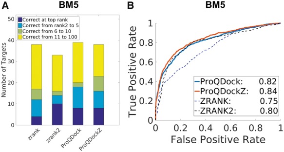
BM5 performance measured by (A) the ability to rank a model with quality acceptable or better among top 1, 5, 10 and 100 and (B) ROC curves; the AUC values are given in the legend
3.4 Test on native structure
Obviously, ProQDock was designed to predict the quality of protein docking models. However, it is also interesting to investigate how they perform on native structures, like a reality check. To this end, ProQDock was calculated for a set of high-resolution native structures in the database DB3 (see Section 2). Indeed, the ProQDock scores for native structures are much higher than the scores obtained for the docking models (with the exception of 'High' quality models) from CnM included as reference (Fig. 5). The median ProQDock for native structures is 0.64 compared with 0.11, 0.31, 0.44 and 0.68 for incorrect, acceptable, medium and high docking model quality, respectively. The high-quality docking models have scores similar to the score for native structures, which makes sense because high-quality models are close to the native structure.
Fig. 5.
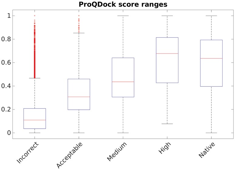
ProQDock score for native structure and incorrect, acceptable, medium and high-quality models from the CnM set
3.5 Complementary of ProQDock and ZRANK2 in ranking correct models
To analyze what features were characteristic to the complementarity behavior of ProQDock and ZRANK2, which resulted in slight but still improved prediction ability of the combined method ProQDockZ, a statistical analysis of features for correct docking models ranked high by ProQDock and not by ZRANK2 (set1) and vice versa (set2) was performed. The sets were constructed by considering the correct models in the MOAL set, up to the point (Fig. 3B) where ProQDock and ZRANK2 intersects corresponding to TPR of 70%, ensuring equal number top correct models before applying the criteria above. ZRANK2 has a fairly strict van der Waals repulsive term and will not be able to rank models with clashes, so the MOAL set was chosen over CnM, as these models have fewer clashes.
Statistics for individual features were calculated as mean and standard deviation of the mean (standard error) for three sets constructed above (Table 3) and feature distributions for correct and incorrect models were calculated (Supplementary Fig. S1). From the statistics, two groups of features can be distinguished based on the set of models selected by ProQDock and ZRANK2, one group (i) with features that are significantly different both in Table 3 as well as from the overall distributions of features of correct models (Supplementary Fig. S1), i.e. a feature has to be significantly different in Table 3 and significantly different from the mean of the overall distribution of correct models, and another group (ii) where features that are invariant.
Table 3.
Feature statistics for highly ranked correct models
| Features | ProQDock (set1) 247 models 50 targets | ZRANK2 (set2) 240 models 39 targets | log10 (Pval) |
|---|---|---|---|
| rGb | 0.031 (±0.001) | 0.031 (±0.002) | −0.3 |
| nBSA | 0.047 (±0.001) | 0.060 (±0.001) | −23.3 |
| Fintres | 0.162 (±0.004) | 0.239 (±0.006) | −26.1 |
| Sc | 0.648 (±0.004) | 0.645 (±0.004) | −0.5 |
| EC | 0.264 (±0.014) | 0.012 (±0.016) | −28.8 |
| ProQ2 | 0.836 (±0.004) | 0.799 (±0.006) | −6.5 |
| Isc | 0.270 (±0.019) | 0.520 (±0.016) | −21.4 |
| rTs | 0.469 (±0.011) | 0.459 (±0.012) | −0.6 |
| Erep | 0.491 (±0.007) | 0.515 (±0.004) | −2.6 |
| Etmr | 0.495 (±0.009) | 0.464 (±0.011) | −1.9 |
| CPM | 0.787 (±0.008) | 0.705 (±0.010) | −9.8 |
| Ld | 0.110 (±0.003) | 0.126 (±0.002) | −4.7 |
| CPscore | 0.359 (±0.018) | 0.224 (±0.009) | −10.4 |
| DockQ | 0.548 (±0.013) | 0.456 (±0.010) | −8.1 |
Descriptive statistics, mean and standard errors of features for set1: correct models ranked by ProQDock and not by ZRANK2; set2: correct models ranked by ZRANK2 and not by ProQDock; from the MOAL set. P-values are calculated using t-test for the difference in mean between set1 and set2. Features in bold are the set of features for which ProQDock and ZRANK2 have significantly different values as defined in group (i) in the text.
The features for which ProQDock and ZRANK2 select models with significantly different ranges of values are (log10(Pval)<-3): nBSA, Fintres, EC, ProQ, Isc, CPM, Ld and CPscore (Table 3). In all cases, except for Ld, at least one of the values is also significantly different from the mean of distribution of correct models (Supplementary Fig. S1, P values not shown). Thus, features in group (i) are EC (0.26 for ProQDock versus 0.01 for ZRANK2), Isc (0.27 versus 0.52, raw unscaled energy term corresponding to −11.6 versus −8.0 in Rosetta Energy Units), CPscore (0.36 versus 0.22), Fintres (0.162 versus 0.239), nBSA (0.047 versus 0.060, note that the scale for nBSA goes from 0 to 0.1), CPM (0.79 versus 0.71) and ProQ2 (0.84 versus 0.80). A common trait to all features in this group (i) is that they all (with the exception of ProQ2) describe the protein–protein interface. nBSA and Fintres measures the relative size of the interface using buried surface area and contacts, respectively; EC describes the electrostatic complementarity of the interface, Isc is the interface energy term in Rosetta, CPscore is an SVM-based measure capturing the composition and contact preferences of different amino acid residues at the interface, and CPM is a composite function of EC, Sc and nBSA (see Section 2). Although, ZRANK2 includes the IFACE potential (which is similar to CPscore) that describe the interface, it is not nearly as detailed as the set of all features listed above. Furthermore, ZRANK2 does not contain an advanced electrostatic term like EC, modeled on fine-grid Poisson–Boltzman continuum electrostatics, which is advantageous over explicit electrostatic models for intrinsically providing equilibrium solutions (Li et al., 2013). This is most likely the reason why many correct models are missed by ZRANK2. On the other hand, it is also possible that ProQDock focus too much on interface features and EC in particular, so it misses many of the correct models with low EC (Supplementary Fig. S1) that ZRANK2 is able to pick up. In fact, a large fraction (21%) of correct models have EC < 0, meaning that they have correlated surface electrostatic potentials (or in other words, unbalanced electric fields) at their interface most likely compensated by stronger constraints of shape complementarity. This is also true for native PPI models (from DB3) where a similar fraction (∼20%) of interfaces had a negative EC, suggesting that EC has much more relaxed thresholds to satisfy compared with Sc (packing), which is a more well-established necessary condition for oligomer formation (Tsuchiya et al., 2006).
The second group (ii) with features that are similar in values attained by models selected by both ProQDock and ZRANK2 (Table 3) are physico-chemical features: rGb, Sc, Erep, rTs, Etmr; all of which have their equivalent representative terms in ZRANK2: rGb is a solvation term, Sc is to some extent captured by the van der Waal’s attractive term, Erep is the van der Waal’s repulsive term, rTs is the total all-atom Rosetta energy (including Erep), Etmr is the rTs excluding the Erep term. Thus, it makes sense that they are not different between the correct models selected by ProQDock or ZRANK2. However, the fact that they are invariant (or stable) suggests that they provide a necessary but not sufficient condition for correct (native like) interaction between two proteins. Hence, they should be treated more as filters, which need to be satisfied. On the other hand, the discriminative (variable) features in group (i) measure specific structural attributes that differ between different sets of correct protein–protein docking models. Finally, it is noteworthy that the overall docking model quality, DockQ, is in fact also markedly better (P < 10 − 8) for models selected only by ProQDock (0.548 ± 0.013) than those selected only by ZRANK2 (0.456 ± 0.010). This is consistent with the observed trends in the discriminating features in both sets.
3.6 A case study of contrasting interface properties by models ranked by ProQDock and ZRANK2
The complementary behavior of ProQDock and ZRANK2 in ranking correct models is further illustrated by two models with contrasting interface properties belonging to the two sets, the first is model a7d from target 1K4C, ranked by ProQDock and not by ZRANK2, and the second is model a1b from target 4CPA, ranked by ZRANK2 and not by ProQDock. Both models were ranked by the combined method ProQDockZ. The models have almost identical overall structural qualities with DockQ score of 0.59 and 0.55, respectively, medium quality according to CAPRI classification. However, they have vastly different values for several features, in particular at the interface. EC, for instance, is completely different (0.76 for ranked by ProQDock versus −0.69 for ranked by ZRANK2) illustrated by the electric fields induced by the different chains on the surfaces (Fig. 6). Also, the Rosetta interface score, Isc, is far better for the model ranked by ProQDock (−21.2 and −4.5 Rosetta Energy Units), which can partly but not fully be explained by the slightly larger interface (56 versus 42 residues) in the two models. In contrast, CPscore is better for the model ranked by ZRANK2 (0.32 versus 0.44) possibly because of the similarity with IFACE term in ZRANK2. Finally, Ld is much higher in the model ranked by ZRANK2 (0.10 versus 0.15) (Note, the Ld distribution is narrow, see Supplementary Fig. S1), revealing that the interface is more connected for the latter (ranked by ZRANK2). However, both models have good shape complementarity at the interface (0.68 in both cases), which, as discussed earlier, is a more necessary condition for inter-protein association, than the electrostatic balance at their interface.
Fig. 6.

Electrostatic Potentials (ESP) mapped onto the molecular interfaces of the model 1K4C-a7d ranked by ProQDock and not by ZRANK2 (A–D), and model 4CPA-a1b ranked by ZRANK2 and not by ProQDock (E–H). In each figure panel (A–H), only one of the two molecular interfaces have been displayed, colored according to its ESP, either owing to the charged atoms of the molecule itself or owing to the partner molecule, while the other partners have been drawn in ribbon. The arrows pointing from a molecule to the surface illustrate from which molecule the ESP is generated. Surface coloring follows deep blue for high positive (10 kT/e) to deep red for high negative (−10 kT/e) ESPs. Ribbons are colored in yellow if the corresponding atoms are charged and dark gray if uncharged (dummy). The high anti-correlated ESP reflected in their contrasting ESP surface coloring leads to a high EC value (0.76) at the interface (compare A-B and C-D). The high correlated ESP reflected in their similar ESP surface coloring leads to a high negative EC value (−0.69) at the interface (compare E-F and G-H). (A and E) ESP mapped onto the interface of the receptor chain, owing to its own charged atoms. (B and F) ESP on the interface of the receptor chain, owing to the charged atoms of the ligand. (C and G) ESP mapped onto the interface of the ligand chain, owing to its own charged atoms. (D and H) ESP on the interface of the ligand chain, owing to the charged atoms of the receptor
This example highlights the difficulty in scoring protein docking models. At one end there are features that serve as critical filters for complex formation, like shape complementarity. On the other hand, there are variations with regard to features like EC, which probably describes the diverse plethora of biological interactions.
4 Conclusions
The aim of this study was to develop a method that could improve the detection of correct docking models in a set of many incorrect docking models. This was done by training SVMs to predict the quality of protein docking models as measured by DockQ using features that can be calculated from the docking model itself. By combining different types of features describing both the protein–protein interface and the overall physical chemistry, it was possible to improve the correlation to DockQ from 0.25 for the best individual features to 0.49. The final version of ProQDock performed better than the state-of-the-art methods ZRANK and ZRANK2 in terms of correlations, ranking and finding correct models on independent test set. Finally, we also demonstrate that it is possible to combine ProQDock with ZRANK and ZRANK2 to improve the overall performance even further. In fact, based on the results described in Sections 3.5 and 3.6, the hybrid method, ProQDockZ should be considered as a better choice over both ProQDock and ZRANK to cover the diverse repertoire of plausible correct protein–protein docking models.
Supplementary Material
Funding
This work was supported by grants from the Swedish Research Council and Swedish e-Science Research Center.
Conflict of Interest: none declared.
References
- Altschul S.F. et al. (1990) Basic local alignment search tool. J. Mol. Biol., 215, 403–410. [DOI] [PubMed] [Google Scholar]
- Anishchenko I. et al. (2014) Protein models: the grand challenge of protein docking. Proteins Struct. Funct. Bioinforma, 82, 278–287. [DOI] [PMC free article] [PubMed] [Google Scholar]
- Banerjee R. et al. (2003) The jigsaw puzzle model: search for conformational specificity in protein interiors. J. Mol. Biol., 333, 211–226. [DOI] [PubMed] [Google Scholar]
- Basu S. et al. (2011) Mapping the distribution of packing topologies within protein interiors shows predominant preference for specific packing motifs. BMC Bioinformatics, 12, 195. [DOI] [PMC free article] [PubMed] [Google Scholar]
- Basu S. et al. (2014a) Applications of complementarity plot in error detection and structure validation of proteins. Indian J. Biochem. Biophys., 51, 188–200. [PubMed] [Google Scholar]
- Basu S. et al. (2014b) SARAMAint: the complementarity plot for protein–protein interface. J. Bioinforma. Intell. Control, 3, 309–314. [Google Scholar]
- Basu S. et al. (2012) Self-complementarity within proteins: bridging the gap between binding and folding. Biophys. J., 102, 2605–2614. [DOI] [PMC free article] [PubMed] [Google Scholar]
- Basu S, Wallner B. (2016) DockQ: a quality measure for protein-protein docking models. Plos One. [DOI] [PMC free article] [PubMed] [Google Scholar]
- Berman H.M. et al. (2000) The protein data bank. Nucleic Acids Res., 28, 235–242. [DOI] [PMC free article] [PubMed] [Google Scholar]
- Bordner A.J., Gorin A.A. (2007) Protein docking using surface matching and supervised machine learning. Proteins, 68, 488–502. [DOI] [PubMed] [Google Scholar]
- Chae M.H. et al. (2010) Predicting protein complex geometries with a neural network. Proteins, 78, 1026–1039. [DOI] [PubMed] [Google Scholar]
- Chang S. et al. (2008) Amino acid network and its scoring application in protein-protein docking. Biophys. Chem., 134, 111–118. [DOI] [PubMed] [Google Scholar]
- Cheng T.M. et al. (2007) pyDock: electrostatics and desolvation for effective scoring of rigid-body protein-protein docking. Proteins, 68, 503–515. [DOI] [PubMed] [Google Scholar]
- Connolly M.L. (1983) Analytical molecular surface calculation. J. Appl. Crystallogr., 16, 548–558. [Google Scholar]
- Cornell W.D. et al. (1995) A second generation force field for the simulation of proteins, nucleic acids, and organic molecules. J. Am. Chem. Soc, 117, 5179–5197. [Google Scholar]
- Dominguez C. et al. (2003) HADDOCK: a protein-protein docking approach based on biochemical or biophysical information. J. Am. Chem, Soc., 125, 1731–1737. [DOI] [PubMed] [Google Scholar]
- Gabb H.A. et al. (1997) Modelling protein docking using shape complementarity, electrostatics and biochemical information. J. Mol. Biol., 272, 106–120. [DOI] [PubMed] [Google Scholar]
- Gao M., Skolnick J. (2011) New benchmark metrics for protein-protein docking methods. Proteins, 79, 1623–1634. [DOI] [PMC free article] [PubMed] [Google Scholar]
- Geppert T. et al. (2010) Protein-protein docking by shape-complementarity and property matching. J Comput Chem, 31, 1919–1928. [DOI] [PubMed] [Google Scholar]
- Glaser F. et al. (2001) Residue frequencies and pairing preferences at protein-protein interfaces. Proteins, 43, 89–102. [PubMed] [Google Scholar]
- Gray J.J. et al. (2003) Protein-protein docking with simultaneous optimization of rigid-body displacement and side-chain conformations. J. Mol. Biol., 331, 281–299. [DOI] [PubMed] [Google Scholar]
- Hubbard S, Thornton J. (1993) NACCESS - Computer Program. Department of Biochemistry and Molecular Biology, University College London. [Google Scholar]
- Hwang H. et al. (2010) Performance of ZDOCK and ZRANK in CAPRI Rounds 13 - 19. Proteins, 78, 3104–3110. [DOI] [PMC free article] [PubMed] [Google Scholar]
- Joachims T. (2002) Learning to Classify Text Using Support Vector Machines. Springer US, Boston, MA. [Google Scholar]
- Khashan R. et al. (2012) Scoring protein interaction decoys using exposed residues (SPIDER): a novel multibody interaction scoring function based on frequent geometric patterns of interfacial residues. Proteins, 80, 2207–2217. [DOI] [PMC free article] [PubMed] [Google Scholar]
- Kryshtafovych A. et al. (2015) Methods of model accuracy estimation can help selecting the best models from decoy sets: assessment of model accuracy estimations in CASP11. Proteins. doi: 10.1002/prot.24919. [DOI] [PMC free article] [PubMed] [Google Scholar]
- Lawrence M.C., Colman P.M. (1993) Shape complementarity at protein/protein interfaces. J. Mol. Biol., 234, 946–950. [DOI] [PubMed] [Google Scholar]
- Lensink M.F. et al. (2007) Docking and scoring protein complexes: CAPRI 3rd Edition. Proteins, 69, 704–718. [DOI] [PubMed] [Google Scholar]
- Lensink M.F., Wodak S.J. (2014) Score_set: a CAPRI benchmark for scoring protein complexes. Proteins, 82, 3163–3169. [DOI] [PubMed] [Google Scholar]
- Li L. et al. (2012) DelPhi: a comprehensive suite for DelPhi software and associated resources. BMC Biophys., 5, 9. [DOI] [PMC free article] [PubMed] [Google Scholar]
- Li L. et al. (2013) On the Dielectric ‘Constant’ of Proteins: Smooth Dielectric Function for Macromolecular Modeling and Its Implementation in DelPhi. J. Chem. Theory Comput., 9, 2126–2136. [DOI] [PMC free article] [PubMed] [Google Scholar]
- Liu S., Vakser I.A. (2011) DECK: distance and environment-dependent, coarse-grained, knowledge-based potentials for protein-protein docking. BMC Bioinformatics, 12, 280. [DOI] [PMC free article] [PubMed] [Google Scholar]
- Lo Conte L. et al. (1999) The atomic structure of protein-protein recognition sites. J. Mol. Biol., 285, 2177–2198. [DOI] [PubMed] [Google Scholar]
- Lyskov S., Gray J.J. (2008) The RosettaDock server for local protein-protein docking. Nucleic Acids Res, 36, W233–W238. [DOI] [PMC free article] [PubMed] [Google Scholar]
- Marillet S. et al. (2016) High-resolution crystal structures leverage protein binding affinity predictions. Proteins, 84, 9–20. [DOI] [PubMed] [Google Scholar]
- McCoy A.J. et al. (1997) Electrostatic complementarity at protein/protein interfaces. J. Mol. Biol., 268, 570–584. [DOI] [PubMed] [Google Scholar]
- Méndez R. et al. (2003) Assessment of blind predictions of protein–protein interactions: current status of docking methods. Proteins, 52, 51–67., [DOI] [PubMed] [Google Scholar]
- Mintseris J. et al. (2007) Integrating statistical pair potentials into protein complex prediction. Proteins, 69, 511–520. [DOI] [PubMed] [Google Scholar]
- Mitra P., Pal D. (2010) New measures for estimating surface complementarity and packing at protein-protein interfaces. FEBS Lett., 584, 1163–1168. [DOI] [PubMed] [Google Scholar]
- Moal I.H. et al. (2013) The scoring of poses in protein-protein docking: current capabilities and future directions. BMC Bioinformatics, 14, 286. [DOI] [PMC free article] [PubMed] [Google Scholar]
- Morik K. et al. (1999) Combining statistical learning with a knowledge-based approach - a case study in intensive care monitoring. In: Proceedings of the Sixteenth International Conference on Machine Learning, ICML ’99. Morgan Kaufmann Publishers Inc., San Francisco, CA, pp. 268–277.
- O’Meara M.J. et al. (2015) Combined covalent-electrostatic model of hydrogen bonding improves structure prediction with Rosetta. J. Chem. Theory Comput, 11, 609–622. [DOI] [PMC free article] [PubMed] [Google Scholar]
- Pierce B., Weng Z. (2008) A combination of rescoring and refinement significantly improves protein docking performance. Proteins, 72, 270–279. [DOI] [PMC free article] [PubMed] [Google Scholar]
- Pierce B., Weng Z. (2007) ZRANK: reranking protein docking predictions with an optimized energy function. Proteins, 67, 1078–1086. [DOI] [PubMed] [Google Scholar]
- Pons C. et al. (2011) Scoring by intermolecular pairwise propensities of exposed residues (SIPPER): a new efficient potential for protein-protein docking. J. Chem. Inf. Model, 51, 370–377. [DOI] [PubMed] [Google Scholar]
- Torchala M. et al. (2013) SwarmDock: a server for flexible protein–protein docking. Bioinformatics, 29, 807–809. [DOI] [PubMed] [Google Scholar]
- Tsuchiya Y. et al. (2006) Analyses of homo-oligomer interfaces of proteins from the complementarity of molecular surface, electrostatic potential and hydrophobicity. Protein Eng. Des. Sel., 19, 421–429. [DOI] [PubMed] [Google Scholar]
- Uziela K, Wallner B. (2016) ProQ2: estimation of model accuracy implemented in Rosetta. Bioinformatics, 32, 1411–1413. [DOI] [PMC free article] [PubMed] [Google Scholar]
- Visscher K.M. et al. (2015) Non-interacting surface solvation and dynamics in protein-protein interactions. Proteins, 83, 445–458. [DOI] [PubMed] [Google Scholar]
- Viswanath S. et al. (2013) Improving ranking of models for protein complexes with side chain modeling and atomic potentials. Proteins, 81, 592–606. [DOI] [PubMed] [Google Scholar]
- Vreven T. et al. (2015) Updates to the Integrated Protein-Protein Interaction Benchmarks: Docking Benchmark Version 5 and Affinity Benchmark Version 2. J. Mol. Biol., 427, 3031–3041. [DOI] [PMC free article] [PubMed] [Google Scholar]
- Winn M.D. et al. (2011) Overview of the CCP4 suite and current developments. Acta Crystallogr. D Biol. Crystallogr., 67, 235–242. [DOI] [PMC free article] [PubMed] [Google Scholar]
- Word J.M. et al. (1999) Asparagine and glutamine: using hydrogen atom contacts in the choice of side-chain amide orientation. J. Mol. Biol., 285, 1735–1747. [DOI] [PubMed] [Google Scholar]
- Xu D., Zhang Y. (2009) Generating triangulated macromolecular surfaces by euclidean distance transform. PLoS ONE, 4, e8140.. [DOI] [PMC free article] [PubMed] [Google Scholar]
Associated Data
This section collects any data citations, data availability statements, or supplementary materials included in this article.